
29. Spectrum Module
The Spectrum module aims at providing support for modeling the frequency-dependent aspects of communications in ns-3. The model was first introduced in [Baldo2009Spectrum], and has been enhanced and refined over the years.
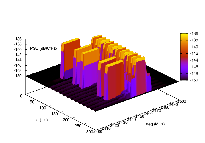
Spectrogram produced by a spectrum analyzer in a scenario
involving wifi signals interfered by a microwave oven, as simulated
by the example adhoc-aloha-ideal-phy-with-microwave-oven.
29.1. Model Description
The module provides:
a set of classes for modeling signals and
a Channel/PHY interface based on a power spectral density signal representation that is technology-independent
two technology-independent Channel implementations based on the Channel/PHY interface
a set of basic PHY model implementations based on the Channel/PHY interface
The source code for the spectrum module is located at src/spectrum.
29.1.1. Design
29.1.1.1. Signal model
The signal model is implemented by the
SpectrumSignalParameters class. This class provides the following
information for a signal being transmitted/received by PHY devices:
a reference to the transmitting PHY device
a reference to the transmitting mobility model, which should be used in StartRx instead of retrieving it from PHY in order to wraparound models to work
a reference to the antenna model used by the transmitting PHY device to transmit this signal
the duration of the signal
the Power Spectral Density (PSD) of the signal, which is assumed to be constant for the duration of the signal
the frequency domain 3D spectrum channel matrix that is needed for MIMO computations when multiple streams are transmitted
the 3D precoding matrix that is needed for MIMO computations when multiple streams are transmitted.
The PSD is represented as a set of discrete scalar values each
corresponding to a certain subband in frequency. The set of frequency subbands
to which the PSD refers to is defined by an instance of the
SpectrumModel class. The PSD itself is implemented as an instance
of the SpectrumValue class which contains a reference to the
associated SpectrumModel class instance. The SpectrumValue
class provides several arithmetic operators to allow to perform calculations
with PSD instances. Additionally, the SpectrumConverter class
provides means for the conversion of SpectrumValue instances from
one SpectrumModel to another.
The frequency domain 3D channel matrix is needed in MIMO systems in which multiple transmit and receive antenna ports can exist, hence the PSD is multidimensional. The dimensions are: the number of receive antenna ports, the number of transmit antenna ports, and the number of subbands in frequency (or resource blocks).
The 3D precoding matrix is also needed in MIMO systems to be able to correctly perform the calculations of the received signal and interference. The dimensions are: the number of transmit antenna ports, the number of transmit streams, and the number of subbands (or resource blocks).
For a more formal mathematical description of the signal model just described, the reader is referred to [Baldo2009Spectrum].
The SpectrumSignalParameters class is meant to include only
information that is valid for all signals; as such, it is not meant to
be modified to add technology-specific information (such as type of
modulation and coding schemes used, info on preambles and reference
signals, etc). Instead, such information shall be put in a new class
that inherits from SpectrumSignalParameters and extends it with
any technology-specific information that is needed. This design
is intended to model the fact that in the real world we have signals
of different technologies being simultaneously transmitted and
received over the air.
29.1.1.2. Channel/PHY interface
The spectrum Channel/PHY interface is defined by the base classes SpectrumChannel
and SpectrumPhy. Their interaction simulates the transmission and
reception of signals over the medium. The way this interaction works is depicted in Sequence diagram showing the interaction between SpectrumPhy and SpectrumChannel:
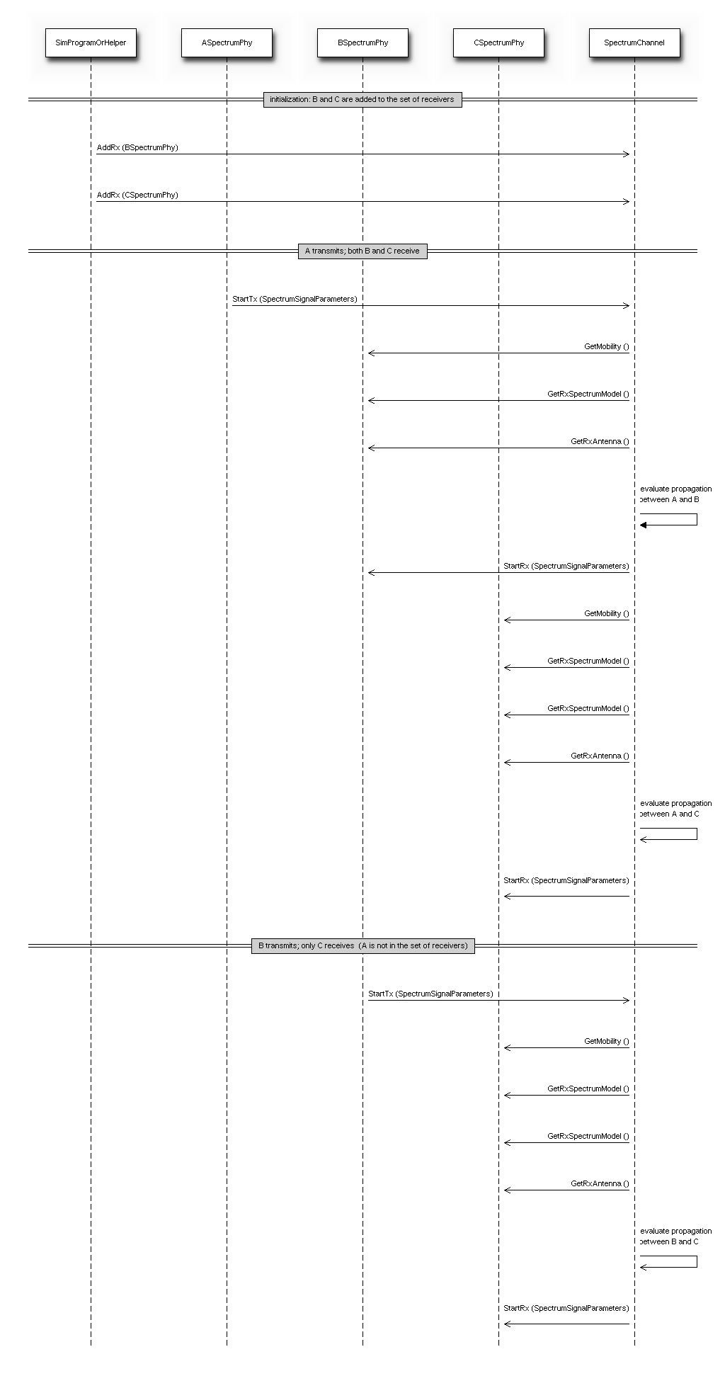
Sequence diagram showing the interaction between SpectrumPhy and SpectrumChannel
29.1.1.3. Spectrum Channel implementations
The module provides two SpectrumChannel implementations:
SingleModelSpectrumChannel and MultiModelSpectrumChannel. They
both provide this functionality:
If a wraparound model is aggregated to the channel, automatically apply it to transmitting nodes.
Propagation loss modeling, in three forms:
you can plug models based on
PropagationLossModelon these channels. Only linear models (where the loss value does not depend on the transmission power) can be used. These models are single-frequency in the sense that the loss value is applied equally to all components of the power spectral density.you can plug models based on
SpectrumPropagationLossModelon these channels. These models can have frequency-dependent loss, i.e., a separate loss value is calculated and applied to each component of the power spectral density.you can plug models based on
PhasedArraySpectrumPropagationLossModelon these channels. These models can have frequency-dependent loss, i.e., a separate loss value is calculated and applied to each component of the power spectral density. Additionally, these models support the phased antenna array at the transmitter and the receiver, i.e., ns-3 antenna typePhasedArrayModel.Propagation delay modeling, by plugging a model based on
PropagationDelayModel. The delay is independent of frequency and applied to the signal as a whole. Delay modeling is implemented by scheduling theStartRxevent with a delay respect to theStartTxevent.
SingleModelSpectrumChannel and MultiModelSpectrumChannel are
quite similar, the main difference is that
MultiModelSpectrumChannel allows to use different
SpectrumModel instances with the same channel instance, by
automatically taking care of the conversion of PSDs among the
different models.
29.1.1.4. Example model implementations
The spectrum module provides some basic implementation of several components that are mainly intended as a proof-of-concept and as an example for building custom models with the spectrum module. Here is a brief list of the available implementations:
SpectrumModel300Khz300GhzLogandSpectrumModelIsm2400MhzRes1Mhzare two exampleSpectrumModelimplementations
HalfDuplexIdealPhy: a basic PHY model using a gaussian interference model (implemented inSpectrumInterference) together with an error model based on Shannon capacity (described in [Baldo2009Spectrum] and implemented inSpectrumErrorModel. This PHY uses theGenericPhyinterface. Its additional custom signal parameters are defined inHalfDuplexIdealPhySignalParameters.
WifiSpectrumValueHelperis an helper object that makes it easy to createSpectrumValuesrepresenting PSDs and RF filters for the wifi technology.
AlohaNoackNetDevice: a minimal NetDevice that allows to send packets overHalfDuplexIdealPhy(or other PHY model based on theGenericPhyinterface). It provides NetDevice trace sourcesMacTx,MacTxDrop,MacRx, andMacPromiscRx.
SpectrumAnalyzer,WaveformGeneratorandMicrowaveOvenare examples of PHY models other than communication devices - the names should be self-explaining.
29.2. Usage
The main use case of the spectrum model is for developers who want to develop a new model for the PHY layer of some wireless technology to be used within ns-3. Here are some notes on how the spectrum module is expected to be used.
SpectrumPhyandSpectrumChannelare abstract base classes. Real code will use classes that inherit from these classes.If you are implementing a new model for some wireless technology of your interest, and want to use the spectrum module, you’ll typically create your own module and make it depend on the spectrum module. Then you typically have to implement:
a child class of
SpectrumModelwhich defines the (sets of) frequency subbands used by the considered wireless technology. Note: instances ofSpectrumModelare typically statically allocated, in order to allow severalSpectrumValueinstances to reference the sameSpectrumModelinstance.a child class of
SpectrumPhywhich will handle transmission and reception of signals (including, if appropriate, interference and error modeling).a child class of
SpectrumSignalParameterswhich will contain all the information needed to model the signals for the wireless technology being considered that is not already provided by the baseSpectrumSignalParametersclass. Examples of such information are the type of modulation and coding schemes used, the PHY preamble format, info on the pilot/reference signals, etc.The available
SpectrumChannelimplementations (SingleModelSpectrumChannelandMultiModelSpectrumChannel, are quite generic. Chances are you can use them as-is. Whether you prefer one or the other it is just a matter of whether you will have a single SpectrumModel or multiple ones in your simulations.Typically, there will be a single SpectrumChannel instance to which several SpectrumPhy instances are plugged. The rule of thumb is that all PHYs that are interfering with each other shall be plugged on the same channel. Multiple SpectrumChannel instances are expected to be used mainly when simulating completely orthogonal channels; for example, when simulating the uplink and downlink of a Frequency Division Duplex system, it is a good choice to use two SpectrumChannel instances in order to reduce computational complexity.
Different types of SpectrumPhy (i.e., instances of different child classes) can be plugged on the same SpectrumChannel instance. This is one of the main features of the spectrum module, to support inter-technology interference. For example, if you implement a WifiSpectrumPhy and a BluetoothSpectrumPhy, and plug both on a SpectrumChannel, then you’ll be able to simulate interference between wifi and bluetooth and vice versa.
Different child classes of
SpectrumSignalParameterscan coexist in the same simulation, and be transmitted over the same channel object. Again, this is part of the support for inter-technology interference. A PHY device model is expected to use theDynamicCast<>operator to determine if a signal is of a certain type it can attempt to receive. If not, the signal is normally expected to be considered as interference.
Many propagation loss and delay models can be added to these channels. The base class
SpectrumChannelprovides anAssignStreams()method to allow the deterministic configuration of random variable stream numbers with a single API call. See the ns-3 Manual chapter on random variables for more information.
29.2.1. Helpers
The helpers provided in src/spectrum/helpers are mainly intended
for the example implementations described in Example model implementations.
If you are developing your custom model based on the
spectrum framework, you will probably prefer to define your own
helpers.
29.2.2. Attributes
Both
SingleModelSpectrumChannelandMultiModelSpectrumChannelhave an attributeMaxLossDbwhich can use to avoid propagating signals affected by very high propagation loss. You can use this to reduce the complexity of interference calculations. Just be careful to choose a value that does not make the interference calculations inaccurate.The example implementations described in Example model implementations also have several attributes.
29.2.3. Output
Both
SingleModelSpectrumChannelandMultiModelSpectrumChannelprovide a trace source calledPathLosswhich is fired whenever a new path loss value is calculated. Note: only single-frequency path loss is accounted for, see the attribute description.The example implementations described in Example model implementations also provide some trace sources.
The helper class
SpectrumAnalyzerHelpercan be conveniently used to generate an output text file containing the spectrogram produced by a SpectrumAnalyzer instance. The format is designed to be easily plotted withgnuplot. For example, if your run the exampleadhoc-aloha-ideal-phy-with-microwave-ovenyou will get an output file calledspectrum-analyzer-output-3-0.tr. From this output file, you can generate a figure similar to Spectrogram produced by a spectrum analyzer in a scenario involving wifi signals interfered by a microwave oven, as simulated by the example adhoc-aloha-ideal-phy-with-microwave-oven. by executing the following gnuplot commands:
unset surface
set pm3d at s
set palette
set key off
set view 50,50
set xlabel "time (ms)"
set ylabel "freq (MHz)"
set zlabel "PSD (dBW/Hz)" offset 15,0,0
splot "./spectrum-analyzer-output-3-0.tr" using ($1*1000.0):($2/1e6):(10*log10($3))
29.2.4. Examples
The example programs in src/spectrum/examples/ allow to see the
example implementations described in Example model implementations in action.
29.2.5. Troubleshooting
Disclaimer on inter-technology interference: the spectrum model makes it very easy to implement an inter-technology interference model, but this does not guarantee that the resulting model is accurate. For example, the gaussian interference model implemented in the
SpectrumInterferenceclass can be used to calculate inter-technology interference, however the results might not be valid in some scenarios, depending on the actual waveforms involved, the number of interferers, etc. Moreover, it is very important to use error models that are consistent with the interference model. The responsibility of ensuring that the models being used are correct is left to the user.
29.3. Testing
In this section we describe the test suites that are provided within the spectrum module.
29.3.1. SpectrumValue test
The test suite spectrum-value verifies the correct functionality of the arithmetic
operators implemented by the SpectrumValue class. Each test case
corresponds to a different operator. The test passes if the result
provided by the operator implementation is equal to the reference
values which were calculated offline by hand. Equality is verified
within a tolerance of  which is to account for
numerical errors.
which is to account for
numerical errors.
29.3.2. SpectrumConverter test
The test suite spectrum-converter verifies the correct
functionality of the SpectrumConverter class. Different test cases
correspond to the conversion of different SpectrumValue instances
to different SpectrumModel instances. Each test passes if the
SpectrumValue instance resulting from the conversion is equal to the reference
values which were calculated offline by hand. Equality is verified
within a tolerance of which is to account for
numerical errors.
Describe how the model has been tested/validated. What tests run in the test suite? How much API and code is covered by the tests? Again, references to outside published work may help here.
29.3.3. Interference test
The test suite spectrum-interference verifies the correct
functionality of the SpectrumInterference and
ShannonSpectrumErrorModel in a scenario involving four
signals (an intended signal plus three interferers). Different test
cases are created corresponding to different PSDs of the intended
signal and different amount of transmitted bytes. The test passes if
the output of the error model (successful or failed) coincides with
the expected one which was determine offline by manually calculating
the achievable rate using Shannon’s formula.
29.3.4. IdealPhy test
The test verifies that AlohaNoackNetDevice and
HalfDuplexIdealPhy work properly when installed in a node. The
test recreates a scenario with two nodes (a TX and a RX) affected by a path loss such
that a certain SNR is obtained. The TX node transmits with a
pre-determined PHY rate and with an application layer rate which is
larger than the PHY rate, so as to saturate the
channel. PacketSocket is used in order to avoid protocol
overhead. Different
test cases correspond to different PHY rate and SNR values. For each
test case, we calculated offline (using Shannon’s formula) whether
the PHY rate is achievable or not. Each test case passes if the
following conditions are satisfied:
if the PHY rate is achievable, the application throughput shall be within
of the PHY rate;
if the PHY rate is not achievable, the application throughput shall be zero.
29.4. Additional Models
29.4.1. TV Transmitter Model
A TV Transmitter model is implemented by the TvSpectrumTransmitter class.
This model enables transmission of realistic TV signals to be simulated and can
be used for interference modeling. It provides a customizable power spectral
density (PSD) model, with configurable attributes including the type of
modulation (with models for analog, 8-VSB, and COFDM), signal bandwidth,
power spectral density level, frequency, and transmission duration. A helper
class, TvSpectrumTransmitterHelper, is also provided to assist users in
setting up simulations.
29.4.1.1. Main Model Class
The main TV Transmitter model class, TvSpectrumTransmitter, provides a
user-configurable PSD model that can be transmitted on the SpectrumChannel.
It inherits from SpectrumPhy and is comprised of attributes and methods to
create and transmit the signal on the channel.
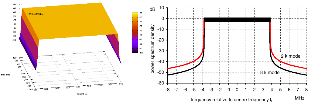
8K COFDM signal spectrum generated from TvSpectrumTransmitter (Left) and
theoretical COFDM signal spectrum [KoppCOFDM] (Right)
One of the user-configurable attributes is the type of modulation for the TV transmitter to use. The options are 8-VSB (Eight-Level Vestigial Sideband Modulation) which is notably used in the North America ATSC digital television standard, COFDM (Coded Orthogonal Frequency Division Multiplexing) which is notably used in the DVB-T and ISDB-T digital television standards adopted by various countries around the world, and analog modulation which is a legacy technology but is still being used by some countries today. To accomplish realistic PSD models for these modulation types, the signals’ PSDs were approximated from real standards and developed into models that are scalable by frequency and power. The COFDM PSD is approximated from Figure 12 (8k mode) of [KoppCOFDM], the 8-VSB PSD is approximated from Figure 3 of [Baron8VSB], and the analog PSD is approximated from Figure 4 of [QualcommAnalog]. Note that the analog model is approximated from the NTSC standard, but other analog modulation standards such as PAL have similar signals. The approximated COFDM PSD model is in 8K mode. The other configurable attributes are the start frequency, signal/channel bandwidth, base PSD, antenna type, starting time, and transmit duration.
TvSpectrumTransmitter uses IsotropicAntennaModel as its antenna model by
default, but any model that inherits from AntennaModel is selectable, so
directional antenna models can also be used. The propagation loss models used
in simulation are configured in the SpectrumChannel that the user chooses to
use. Terrain and spherical Earth/horizon effects may be supported in future ns-3
propagation loss models.
After the attributes are set, along with the SpectrumChannel,
MobilityModel, and node locations, the PSD of the TV transmitter signal can
be created and transmitted on the channel.
29.4.1.2. Helper Class
The helper class, TvSpectrumTransmitterHelper, consists of features to
assist users in setting up TV transmitters for their simulations. Functionality
is also provided to easily simulate real-world scenarios.
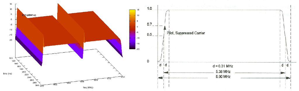
North America ATSC channel 19 & 20 signals generated using
TvSpectrumTransmitterHelper (Left) and theoretical 8-VSB signal
[Baron8VSB] (Right). Note that the theoretical signal is not shown in dB
while the ns-3 generated signals are.
Using this helper class, users can easily set up TV transmitters right after configuring attributes. Multiple transmitters can be created at a time. Also included are real characteristics of specific geographic regions that can be used to run realistic simulations. The regions currently included are North America, Europe, and Japan. The frequencies and bandwidth of each TV channel for each these regions are provided.
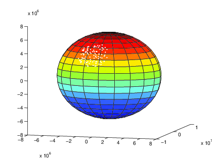
Plot from MATLAB implementation of CreateRegionalTvTransmitters method in
TvSpectrumTransmitterHelper. Shows 100 random points on Earth’s surface
(with altitude 0) corresponding to TV transmitter locations within a 2000 km
radius of 35° latitude and -100° longitude.
A method (CreateRegionalTvTransmitters) is provided that enables users to randomly generate multiple TV transmitters from a specified region with a given density within a chosen radius around a point on Earth’s surface. The region, which determines the channel frequencies of the generated TV transmitters, can be specified to be one of the three provided, while the density determines the amount of transmitters generated. The TV transmitters’ antenna heights (altitude) above Earth’s surface can also be randomly generated to be within a given maximum altitude. This method models Earth as a perfect sphere, and generated location points are referenced accordingly in Earth-Centered Earth-Fixed Cartesian coordinates. Note that bodies of water on Earth are not considered in location point generation–TV transmitters can be generated anywhere on Earth around the origin point within the chosen maximum radius.
29.4.1.3. Examples
Two example simulations are provided that demonstrate the functionality of the
TV transmitter model. tv-trans-example simulates two 8-VSB TV transmitters
with adjacent channel frequencies. tv-trans-regional-example simulates
randomly generated COFDM TV transmitters (modeling the DVB-T standard)
located around the Paris, France area with channel frequencies and bandwidths
corresponding to the European television channel allocations.
29.4.1.4. Testing
The tv-spectrum-transmitter test suite verifies the accuracy of the
spectrum/PSD model in TvSpectrumTransmitter by testing if the maximum power
spectral density, start frequency, and end frequency comply with expected values
for various test cases.
The tv-helper-distribution test suite verifies the functionality of the
method in TvSpectrumTransmitterHelper that generates a random number of TV
transmitters based on the given density (low, medium, or high) and maximum
number of TV channels. It verifies that the number of TV transmitters generated
does not exceed the expected bounds.
The CreateRegionalTvTransmitters method in TvSpectrumTransmitterHelper
described in Helper Class uses two methods from the
GeographicPositions class in the Mobility module to generate the random
Cartesian points on or above earth’s surface around an origin point which
correspond to TV transmitter positions. The first method converts Earth
geographic coordinates to Earth-Centered Earth-Fixed (ECEF) Cartesian
coordinates, and is tested in the geo-to-cartesian test suite by comparing
(with 10 meter tolerance) its output with the output of the geographic to ECEF
conversion function [MatlabGeo] of the MATLAB Mapping Toolbox for numerous
test cases. The other used method generates random ECEF Cartesian points around
the given geographic origin point, and is tested in the rand-cart-around-geo
test suite by verifying that the generated points do not exceed the given
maximum distance radius from the origin point.
29.4.2. 3GPP TR 38.901 fast fading model
The framework described by TR 38.901 [TR38901] is a 3D statistical Spatial
Channel Model supporting different propagation environments (e.g., urban,
rural, indoor), multi-antenna operations and the modeling of wireless channels
between 0.5 and 100 GHz.
The overall channel is represented by the matrix  , in which each
entry H u,s
, in which each
entry H u,s  corresponds to the impulse response of the channel between the
s-th element of the transmitting antenna and the u-th element of the receiving
antenna. H u,s is generated by the superposition of N different multi-path
components, called clusters, each of which composed of M different rays.
The channel matrix generation procedure accounts for large and small scale
propagation phenomena. The classes
corresponds to the impulse response of the channel between the
s-th element of the transmitting antenna and the u-th element of the receiving
antenna. H u,s is generated by the superposition of N different multi-path
components, called clusters, each of which composed of M different rays.
The channel matrix generation procedure accounts for large and small scale
propagation phenomena. The classes ThreeGppSpectrumPropagationLossModel and
ThreeGppChannelModel included in the spectrum module take care of the generation
of the channel coefficients and the computation of the frequency-dependent
propagation loss.
29.4.2.1. Implementation
Our implementation is described in [Zugno]. It is based on the model described
in [Zhang], but the code has been refactored, extended, and aligned to TR 38.901
[TR38901].
The fundamental assumption behind this model is the channel reciprocity, i.e.,
the impulse response of the channel between node a and node b is the same as
between node b and node a.
To deal with the equivalence of the channel between a and b, no matter who is
the transmitter and who is the receiver, the model considers the pair of nodes
to be composed by one “s” and one “u” node. The channel matrix, as well as other
parameters, are saved and used under the assumption that, within a pair, the
definition of the “s” and “u” node will always be the same. For more details,
please have a look at the documentation of the classes
ThreeGppChannelModel and ThreeGppSpectrumPropagationLossModel.
Note:
Since ns-3.47, the model includes an update technique aligned with the 3GPP TR 38.901 spatial-consistency procedure (see [TR38901], Sec. 7.6.3), based on Procedure A (Sec. 7.6.3.2). The channel-parameter evolution follows the Procedure A update equations to preserve correlation across consecutive channel evaluations, while the criteria for when to apply an update are adapted for ns-3’s discrete-event operation (i.e., updates are triggered when the channel is evaluated and the configured
UpdatePeriodhas elapsed; if the maximum distance the BS and/or UT traveled between evaluations exceeds the 1 m step-size constraint, the model falls back to re-generating channel parameters and thus the channel matrix). Drop-based spatial consistency across multiple initial locations (Sec. 7.6.3.1) and Procedure B are not implemented.Issue regarding the blockage model: according to 3GPP TR 38.901 v15.0.0 (2018-06) section 7.6.4.1, the blocking region for self-blocking is provided in LCS. However, here, clusterAOA and clusterZOA are in GCS and blocking check is performed for self-blocking similar to non-self blocking, that is in GCS. One would expect the angles to be transposed to LCS before checking self-blockage.
No error model is provided in this module; a link-to-system campaign may be needed to incorporate it in existing modules.
29.4.2.2. ThreeGppSpectrumPropagationLossModel
The class ThreeGppSpectrumPropagationLossModel implements the
PhasedArraySpectrumPropagationLossModel interface and enables the modeling of frequency
dependent propagation phenomena while taking into account the specific pair of the
phased antenna array at the transmitter and the receiver. The main method is
DoCalcRxPowerSpectralDensity, which takes as input the SpectrumSignalParameters
structure, which contains, among others, the power spectral density (PSD) of the
transmitted signal, and the precoding matrix of the transmitter which is needed
for MIMO computations. Other input parameters are the mobility models of the
transmitting and receiving node, and the phased antenna array of the
transmitting and receiving node.
DoCalcRxPowerSpectralDensity computes the PSD of the received signal
(used in case of single stream transmission), and the frequency domain 3D
channel matrix between receive and transmit antenna ports (needed for MIMO
computations when multiple streams are transmitted).
Finally, it returns the SpectrumSignalParameters which contains the
received PSD and the frequency domain 3D spectrum channel matrix.
Procedure used to compute the PSD of the received signal and the frequency domain 3D spectrum channel matrix:
1. Retrieve the beamforming vectors
To account for the beamforming, ThreeGppSpectrumPropagationLossModel has to
retrieve the beamforming vectors of the transmitting and receiving antennas.
The method DoCalcRxPowerSpectralDensity uses the antenna objects
that are passed as parameters for both the transmitting and receiving devices,
and calls the method GetBeamformingVector to retrieve the beamforming vectors
of these antenna objects.
2. Retrieve the channel matrix and the channel params
The ThreeGppSpectrumPropagationLossModel relies on the ThreeGppChannelModel class
to obtain the channel matrix and channel parameters.
In particular, it makes use of the method GetChannel,
which returns a ChannelMatrix object containing the channel
matrix, the generation time, the node pair, and the phased antenna array pair among
which is created this channel matrix.
Additionally, it makes use of the method GetParams which
returns a ChannelParams object containing the channel parameters.
Notice that the channel information is split into these two structures
(ChannelMatrix and ChannelParams) to support multiple collocated phased antenna arrays at
TX/RX node. ChannelParams (also its specialization ThreeGppChannelParams structure)
contains parameters which are common for all the channels among
the same RX/TX node pair, while ChannelMatrix contains the channel matrix for the specific pair
of the phased antenna arrays of TX/RX nodes.
For example, if the TX and the RX node have multiple collocated antenna arrays,
then there will be multiple channel matrices among this pair of nodes for different pairs
of antenna arrays of the TX and the RX node.
These channel matrices that are among the same pair of nodes have common channel parameters,
i.e., they share the same channel condition, cluster powers, cluster delays,
AoD, AoA, ZoD, ZoA, K_factor, delay spread, etc.
On the other hand, each pair of TX and RX antenna arrays has a specific channel matrix
and fading, which depends on the actual antenna element positions and field patterns of
each pair of antenna array subpartitions.
The ThreeGppChannelModel instance is automatically
created in the ThreeGppSpectrumPropagationLossModel constructor and it can
be configured by using the method SetChannelModelAttribute.
Notice that in MultiModelSpectrumChannel it is checked whether the TX/RX
SpectrumPhy instances belong to different TX/RX nodes.
This is needed to avoid pathloss models calculations among
the phased antenna arrays of the same node, because there are no models yet
in ns-3 that support the calculation of this kind of interference.
4. Compute the long term component
The method GetLongTerm returns the long term component obtained by multiplying
the channel matrix and the beamforming vectors. The function CalculateLongTermComponent
calculates the long term component per RX and TX port pair. Finally, GetLongTerm
returns a 3D long term channel matrix whose dimensions are the number of the
receive antenna ports, the number transmit antenna ports, and
the number of clusters. When multiple ports are being configured note that
the sub-array partition model is adopted for TXRU virtualization, as described
in Section 5.2.2 of 3GPP TR 36.897 [TR36897], and so equal beam weights are used for all the ports.
Support of the full-connection model for TXRU virtualization would need extensions.
To reduce the computational load, the long term
components associated to the different channels are stored in the m_longTermMap
and recomputed only if the associated channel matrix is updated or if the
transmitting and/or receiving beamforming vectors have changed. Given the channel
reciprocity assumption, for each node pair a single long term component is saved in the map.
5. Apply the small scale fading, calculate the channel gain, generate the
frequency domain 3D spectrum channel matrix, and finally compute the received PSD
The method CalcBeamformingGain computes the channel gain in each sub-band and
applies it to the PSD of the transmitted signal to obtain the received PSD.
To compute the sub-band gain, it accounts for the Doppler phenomenon and the
time dispersion effect on each cluster.
In order to reduce the computational load, the Doppler component of each
cluster is computed considering only the central ray.
Also, as specified here, it is possible to account for
the effect of environmental scattering following the model described in Sec. 6.2.3
of 3GPP TR 37.885.
This is done by deviating the Doppler frequency by a random value, whose
distribution depends on the parameter  .
The value of can be configured using the attribute “vScatt”
(by default it is set to 0, so that the scattering effect is not considered).
Function
.
The value of can be configured using the attribute “vScatt”
(by default it is set to 0, so that the scattering effect is not considered).
Function GenSpectrumChannelMatrix generates the received PSD for each pair of
the transmit and receive antenna ports. It creates a frequency domain 3D spectrum
channel matrix whose dimensions are the number of receive antenna ports,
the number of transmit antenna ports, and the number of resource blocks.
Finally, the frequency domain 3D spectrum channel matrix is used to obtain the
received PSD. In case of multiple ports at the transmitter the PSD is calculated
by summing per each RB the real parts of the diagonal elements of the (H*P)^h * (H*P),
where H is the frequency domain spectrum channel matrix and P is the precoding matrix.
29.4.2.3. ThreeGppChannelModel
The class ThreeGppChannelModel implements the channel matrix generation procedure described in
3GPP TR 38.901 [TR38901] and an update technique aligned with 3GPP TR 38.901 spatial-consistency
feature (Procedure A), with ns-3-specific update triggering criteria suited to discrete-event simulation.
The main method is GetChannel, which takes as input the mobility models of
the transmitter and receiver nodes, the associated antenna objects,
and returns a ChannelMatrix object containing:
the channel matrix of size UxSxN, where U is the number of receiving antenna elements, S is the number of transmitting antenna elements and N is the number of clusters
the clusters delays, as an array of size N
the clusters arrival and departure angles, as a 2D array in which each row corresponds to a direction (AOA, ZOA, AOD, ZOD) and each column corresponds to a different cluster
a time stamp indicating the time at which the channel matrix was generated
the node IDs
other channel parameters
The ChannelMatrix objects are cached per link in the map m_channelMatrixMap.
A new channel realization (i.e., a new ChannelMatrix generated from newly
generated channel parameters) is created when:
the channel condition for the link changes (e.g., LOS/NLOS and/or O2I transitions), as reported by the configured channel-condition model; or
the antenna-array configuration changes (e.g., number of antenna elements/ports), since this changes the required matrix dimensions.
spatial-consistency updates are enabled (
UpdatePeriodis nonzero) and an update attempt observes a maximum endpoint displacement > 1 m (exceeding the Procedure A step-size constraint), the model re-generates channel parameters (and thus the channel matrix).
If spatial-consistency updates are enabled and the 1 m step-size constraint is
satisfied, the cached channel parameters are updated (Procedure A), and the
ChannelMatrix is recomputed from the updated parameters (without drawing a
new independent realization).
The channel condition is provided by the configured channel-condition model, which
may be time-varying (e.g., stochastic blockage) and may be evaluated/updated
according to its own internal logic (potentially with its own periodicity),
independent of the small-scale fading evolution modeled in the
ThreeGppChannelModel. The channel condition may change regardless of whether
the nodes are static or mobile.
Antenna-parameter changes are expected to be rare; one example is NR initial access/attachment, where a simplified receiver configuration may be assumed during attachment and then restored to the user-configured antenna array, triggering a matrix regeneration.
The ChannelMatrix itself does not depend on beamforming. Beamforming
vectors (and the precoding matrix) are applied later in
ThreeGppSpectrumPropagationLossModel::DoCalcRxPowerSpectralDensity when
computing the long-term component and the received PSD (see the procedure in
ThreeGppSpectrumPropagationLossModel above). Beamforming weights may change
at each reception/transmission without forcing regeneration of the cached
ChannelMatrix.
The propagation scenario and the operating frequency can be configured through
the Scenario and Frequency attributes, respectively.
Spatial-consistency evolution aligned with 3GPP TR 38.901 Procedure A update
equations is enabled when the UpdatePeriod attribute is set to a
non-zero value (see below).
Spatial consistency procedure: The spatial consistency update technique is aligned with 3GPP TR 38.901 Sec. 7.6.3.2 (Procedure A). Procedure A aims to preserve spatial correlation of cluster-specific random terms across consecutive channel evaluations as nodes move (e.g., cluster delays from Fig. 7.5-1, Step 5; the per-cluster shadowing term used in the cluster-power computation; and the random offsets/signs used for AOD/AOA/ZOD/ZOA generation in Step 7).
In ns-3, the channel-parameter evolution follows the Procedure A update equations,
while the update-triggering criteria are adapted to a discrete-event simulation
environment. In TR 38.901, Procedure A is described for updates at about 1 m
granularity, without prescribing a discrete evaluation schedule, and there is no
specified time or distance at which a new channel realization is drawn;
in ns-3, updates are attempted when the channel is evaluated and the configured
UpdatePeriod has elapsed, and the model enforces the 1 m step-size constraint
(falling back to re-generation of channel parameters when it is exceeded).
With Procedure A, large-scale parameters evolve as a first-order, spatially correlated stochastic process. Continuity is obtained by evolving a cached channel state over time/distance; no position-indexed channel field is defined. As a consequence, the channel is trajectory-dependent, and revisiting the same location does not necessarily reproduce the exact same channel realization. This behavior is consistent with the stochastic modeling approach defined in TR 38.901 [TR38901]. Users requiring strict position-based repeatability (including under LOS/NLOS state changes driven by the channel-condition model) would have to implement a map/field-based approach (e.g., spatially correlated LSP maps in WINNER-derived frameworks such as QuaDRiGa) [WIN2D112] [QUADRIGA] or an explicitly position-seeded regeneration policy.
Drop-based spatial consistency across multiple initial locations (TR 38.901 Sec. 7.6.3.1) and Procedure B (TR 38.901 Sec. 7.6.3.2) are not implemented in this model.
The initial channel realization for a link is generated using the standard 3GPP cluster/ray generation procedure (Fig. 7.5-1). Spatial consistency is then introduced through subsequent Procedure A updates of the same link. During each update attempt, Procedure A updates the channel parameters in a cluster-wise manner. First, cluster delays are updated according to Eq. 7.6-9 in [TR38901]. Second, cluster powers are updated using the updated cluster delays; during this step, the per-cluster shadowing term is evolved (not re-generated) based on the correlation distance of the configured scenario. Third, cluster departure and arrival angles are updated using the UT/BS motion information, as defined in Eqs. 7.6-10b and 7.6-10c and the subsequent angle-update equations in Eqs. 7.6-11 to 7.6-14.
In ns-3, the update period is defined by UpdatePeriod and is analogous to
 in TR 38.901 Sec. 7.6.3.2. When the channel is evaluated and
UpdatePeriod has elapsed since the last parameter generation/update,
the model proceeds as follows:
If the maximum endpoint displacement since the last parameter generation/update is within 1 m, the model applies Procedure A updates to obtain a spatially consistent channel evolution.
If the maximum endpoint displacement is greater than 1 m, the model re-generates the channel parameters (and thus the channel matrix) instead of applying Procedure A for that update step.
The small update distance is consistent with the intent of Procedure A to evolve small-scale channel parameters smoothly as the terminal moves; larger displacements between evaluations are handled by re-generation rather than attempting to extrapolate multiple intermediate updates.
Note on the 1 m update distance vs. correlation distances: The 1 m rule is a
step-size constraint for applying Procedure A updates (i.e., the model updates
the channel in small spatial increments). It does not imply that the channel is
only correlated over 1 m. The scenario correlation distances provided in TR 38.901
Table 7.6.3.1-2 parameterize the rate at which cluster-level random variables
(e.g., per-cluster shadowing) decorrelate with displacement across successive
updates, via an exponential correlation function (TR 38.901, Eq. 7.4-5) of the form
 . Consequently, when Procedure A is
applied repeatedly over many small steps, variables can remain correlated over
tens of meters when
. Consequently, when Procedure A is
applied repeatedly over many small steps, variables can remain correlated over
tens of meters when  is large, even though each individual update
step is limited to 1 m.
is large, even though each individual update
step is limited to 1 m.
Design note (displacement > 1 m and update triggering): TR 38.901 recommends
choosing such that the displacement between successive updates
remains within 1 m (often expressed as  ).
In link-/physical-level channel simulators, the channel is commonly evolved at a
fixed update distance/period along a user trajectory (e.g., NYUSIM) [NYUSIM].
In a system-level simulator, however, forcing periodic channel updates even when
the link is not used (no traffic, no transmissions) may be computationally
expensive in large-scale simulations.
).
In link-/physical-level channel simulators, the channel is commonly evolved at a
fixed update distance/period along a user trajectory (e.g., NYUSIM) [NYUSIM].
In a system-level simulator, however, forcing periodic channel updates even when
the link is not used (no traffic, no transmissions) may be computationally
expensive in large-scale simulations.
Since ns-3 is a discrete-event simulator, channel evaluations may occur at irregular times (e.g., sparse or bursty traffic), and an update attempt may observe a displacement larger than 1 m. In that situation, several behaviors are possible: (i) keep the previous channel state without updating, (ii) re-generate a new realization, (iii) approximate the motion by splitting the interval into smaller steps and applying multiple updates, or (iv) force periodic channel updates independent of traffic (i.e., drive the evolution from a dedicated timer and update internal state even when the channel is not queried).
Option (i) avoids discontinuities but may keep the channel unchanged over large displacements. Option (ii) is conservative and simple, but introduces a new realization when the update-distance constraint is exceeded. Option (iii) would require assumptions about the intermediate trajectory (only start/end positions are known) and increases computational cost. Option (iv) may also be computationally expensive in large-scale simulations, since it updates channels even when the channel is not evaluated.
ns-3 chooses option (ii) as a fallback: if the displacement exceeds 1 m at an update instant, the channel parameters are re-generated.
How to choose ``UpdatePeriod``. To obtain Procedure A updates (rather than
frequent re-generation), UpdatePeriod should be selected so that the expected
maximum endpoint displacement stays below 1 m between updates, i.e.,
 .
.
Example: if the maximum expected endpoint speed is 5 m/s, choosing
UpdatePeriod <= 0.2 s keeps the maximum endpoint displacement below 1 m.
Important: UpdatePeriod sets a minimum interval between successive
channel updates; the channel state is updated only when the channel is evaluated,
so the effective update instants are traffic-driven (e.g., receptions/transmissions
or other events that require channel evaluation). For mobile scenarios,
users should ensure that the channel is evaluated at least as often as UpdatePeriod
(e.g., by periodic transmissions/receptions, control signaling, or application traffic).
Otherwise, spatial-consistency updates may be skipped and the model may fall back to
re-generation after larger displacements.
If the channel is not evaluated for longer than UpdatePeriod, then the next
evaluation triggers an update attempt based on the current displacement since
the last generation/update (Procedure A if within 1 m, otherwise re-generation).
The following rule-of-thumb values illustrate a recommended upper bound for
UpdatePeriod to keep the maximum endpoint displacement within 1 m. Users should also
ensure that the channel is evaluated at least that often (e.g., via periodic
signaling or traffic), otherwise updates may be skipped.
Speed (km/h) |
Speed (m/s) |
Max |
Recommended channel-evaluation / signaling period (ms) |
|---|---|---|---|
3 |
0.833 |
1200 |
<= 1200 |
30 |
8.33 |
120 |
<= 120 |
60 |
16.67 |
60 |
<= 60 |
For links where both endpoints move (e.g., V2V), two different “displacements” are relevant:
The maximum endpoint displacement (max motion of either endpoint since the last generation/update) is used to enforce the 1 m step-size constraint for applying Procedure A.
The relative (geometry) displacement (change in the Tx–Rx relative position vector) is used as the displacement input for correlation updates of cluster-level random terms (e.g., the per-cluster shadowing term used in the cluster power update).
For Procedure A, several cluster-level random terms are evolved as functions of displacement between consecutive updates, using exponential spatial correlation models (e.g., [TR38901], Eq. 7.4-5). In TR 38.901 the procedure is described from the perspective of a moving terminal; when both endpoints move (e.g., V2V), ns-3 generalizes the triggering constraint by using the maximum displacement of either endpoint since the last generation/update (maximum endpoint displacement), while still using the change of the Tx–Rx relative position vector (relative/geometry displacement) as the displacement input for correlation updates of cluster-level random terms (e.g., the per-cluster shadowing term used in the cluster power update).
Thus, vehicles traveling in the same direction at similar speeds may have a small
relative (geometry) displacement (slow geometry evolution), even though the
maximum endpoint displacement can be large and may force a smaller UpdatePeriod
to avoid exceeding the 1 m step-size constraint.
Note that relative (geometry) displacement close to zero does not necessarily
mean that no update occurs. Procedure A includes update components that are
driven by endpoint motion over (in ns-3, UpdatePeriod
is the analogue of ), in addition to components that use
displacement-dependent spatial correlation. For example, the per-cluster delay
evolution uses endpoint velocity terms over (see [TR38901],
Eq. 7.6-9). Cluster-angle updates also use the endpoint motion through the
rotation/velocity terms (see [TR38901], Eqs. 7.6-10b and 7.6-10c) and the
subsequent angle-update equations (Eqs. 7.6-11 to 7.6-14). Therefore, even in
scenarios where the Tx–Rx geometry changes slowly (e.g., near-parallel motion),
ns-3 may still perform a Procedure A update when UpdatePeriod expires
(subject to the 1 m step-size constraint), and motion-/time-dependent
components (e.g., angle evolution and related Doppler/phase terms) may still
evolve. In contrast, updates that explicitly take the relative/geometry
displacement as input (e.g., per-cluster shadowing correlation via the
exponential model in [TR38901], Eq. 7.4-5) will exhibit little or no change when
the relative/geometry displacement is near zero.
Example (V2V, same direction): v1 = 120 km/h, v2 = 100 km/h, so the relevant
speed for the 1 m step-size constraint is the maximum endpoint speed,
 km/h = 33.3 m/s. To keep the
maximum endpoint displacement below 1 m between updates, choose
km/h = 33.3 m/s. To keep the
maximum endpoint displacement below 1 m between updates, choose
UpdatePeriod <= 30 ms and ensure the channel is evaluated (e.g., via periodic
signaling/traffic) with a period <= 30 ms.
Channel consistency applicability: The correlation distances used by the
Procedure A updates depend on the configured scenario. For terrestrial cellular
scenarios such as UMa, UMi, RMa, and Indoor, the spatial correlation distances
used for per-cluster shadowing updates are specified in 3GPP TR 38.901 (see
Table 7.6.3.1-2, “Correlation distance for spatial consistency”) and are
reflected in the corresponding 3GPP parameter tables of the ThreeGppChannelModel.
For other scenarios, such as V2V and NTN, the relevant 3GPP technical reports
(e.g., TR 37.885 for V2X and TR 38.811 for NTN) describe channel models and
mobility assumptions but do not provide standardized tables for cluster
correlation distances comparable to those in TR 38.901. Consequently, while the
spatial consistency procedure can be used when these scenarios are configured,
users should be aware that appropriate correlation-distance values must be
selected and configured in the ThreeGppChannelModel parameter tables based
on the intended deployment and propagation environment. In the absence of
standardized 3GPP values, the current implementation uses a short correlation
distance (1 m) for per-cluster shadowing, resulting in weak spatial correlation
unless configured otherwise.
Blockage model: 3GPP TR 38.901 also provides an optional
feature that can be used to model the blockage effect due to the
presence of obstacles, such as trees, cars or humans, at the level
of a single cluster. This differs from a complete blockage, which
would result in an LOS to NLOS transition. Therefore, when this
feature is enabled, an additional attenuation is added to certain
clusters, depending on their angle of arrival. There are two possible
methods for the computation of the additional attenuation, i.e.,
stochastic (Model A) and geometric (Model B). In this work, we
used the implementation provided by [Zhang], which
uses the stochastic method. In particular, the model is implemented by the
method CalcAttenuationOfBlockage, which computes the additional attenuation.
The blockage feature can be disable through the attribute “Blockage”. Also, the
attributes “NumNonselfBlocking”, “PortraitMode” and “BlockerSpeed” can be used
to configure the model.
29.4.2.4. Testing
The test suite ThreeGppChannelTestSuite includes five test cases:
ThreeGppChannelMatrixComputationTestchecks if the channel matrix has the correct dimensions and if it correctly normalizedThreeGppChannelMatrixUpdateTest, which checks if the channel matrix is correctly updated when the coherence time exceedsThreeGppSpectrumPropagationLossModelTest, which tests the functionalities of the classThreeGppSpectrumPropagationLossModel. It builds a simple network composed of two nodes, computes the power spectral density received by the receiving node, andChecks if the long term components for the direct and the reverse link are the same,
Checks if the long term component is updated when changing the beamforming vectors,
Checks if the long term is updated when changing the channel matrix
ThreeGppCalcLongTermMultiPortTest, which tests that the channel matrices are correctly generated when multiple transmit and receive antenna ports are used.ThreeGppMimoPolarizationTest, which tests that the channel matrices are correctly generated when dual-polarized antennas are being used.ThreeGppChannelConsistencyTestis designed to verify that consecutive channel realizations remain spatially consistent while the user is moving, which is the scenario addressed by the implemented channel consistency Procedure A (3GPP TR 38.901, Sec. 7.6.3).The test considers both LOS and NLOS conditions, thereby exercising the different channel update mechanisms defined for each case, in particular the cluster delay update (Eq. 7.6-9) and the cluster departure and arrival angle updates (Eqs. 7.6-10b and 7.6-10c). Multiple test cases are defined for different carrier frequencies and user speeds. For each test case, the channel coherence time is computed and the channel update period (configured through the UpdatePeriod attribute) is set accordingly.
The test verifies that spatially consistent channel updates produce significantly smoother channel evolution (approximately five times smaller variations) compared to generating independent channel realizations under the same LOS/NLOS conditions. To evaluate channel consistency, several metrics are tracked, including per-cluster parameters such as cluster delay, cluster power, and cluster angles (AOA and ZOA), as well as a global channel metric, the Frobenius norm of the channel matrix. For the per-cluster analysis, the third cluster, as defined in Table 7.8.5 for channel consistency calibration, is selected.
Note: TR 38.901 includes a calibration procedure that can be used to validate the model, but it requires some additional features which are not currently implemented, thus is left as future work.
29.4.2.5. References
- Baron8VSB(1,2)
Baron, Stanley. “First-Hand:Digital Television: The Digital Terrestrial Television Broadcasting (DTTB) Standard.” IEEE Global History Network. <http://www.ieeeghn.org/wiki/index.php/First-Hand:Digital_Television:_The_Digital_Terrestrial_Television_Broadcasting_(DTTB)_Standard>.
- KoppCOFDM(1,2)
Kopp, Carlo. “High Definition Television.” High Definition Television. Air Power Australia. <http://www.ausairpower.net/AC-1100.html>.
- MatlabGeo
“Geodetic2ecef.” Convert Geodetic to Geocentric (ECEF) Coordinates. The MathWorks, Inc. <http://www.mathworks.com/help/map/ref/geodetic2ecef.html>.
- QualcommAnalog
Stephen Shellhammer, Ahmed Sadek, and Wenyi Zhang. “Technical Challenges for Cognitive Radio in the TV White Space Spectrum.” Qualcomm Incorporated.
- TR38901(1,2,3,4,5,6,7,8,9,10,11,12,13,14,15,16,17,18)
3GPP. 2018. TR 38.901. Study on channel for frequencies from 0.5 to 100 GHz. V.15.0.0. (2018-06).
- NYUSIM
Shihao Ju and Theodore S. Rappaport. “Simulating Motion - Incorporating Spatial Consistency into the NYUSIM Channel Model.” NYU WIRELESS.
- WIN2D112
IST-4-027756 WINNER II, Deliverable D1.1.2, “WINNER II channel models: Part I - Channel models”, 2007. Available at: https://signserv.signal.uu.se/Publications/WINNER/WIN2D112.pdf
- QUADRIGA
S. Jaeckel, L. Raschkowski, K. Börner, and L. Thiele, “QuaDRiGa: Quasi Deterministic Radio Channel Generator - User Manual and Documentation”, Fraunhofer HHI. Available at: https://quadriga-channel-model.de/wp-content/uploads/2015/02/quadriga_documentation_v1.2.3.pdf
- Zhang(1,2)
Menglei Zhang, Michele Polese, Marco Mezzavilla, Sundeep Rangan, Michele Zorzi. “ns-3 Implementation of the 3GPP MIMO Channel Model for Frequency Spectrum above 6 GHz”. In Proceedings of the Workshop on ns-3 (WNS3 ‘17). 2017.
- Zugno
Tommaso Zugno, Michele Polese, Natale Patriciello, Biljana Bojovic, Sandra Lagen, Michele Zorzi. “Implementation of a Spatial Channel Model for ns-3”. Submitted to the Workshop on ns-3 (WNS3 ‘20). 2020. Available: https://arxiv.org/abs/2002.09341
- TR36897
3GPP. 2015. TR 36.897. Study on elevation beamforming / Full-Dimension (FD) Multiple Input Multiple Output (MIMO) for LTE. V13.0.0. (2015-06)
29.4.3. Two-Ray fading model
The model aims to provide a performance-oriented alternative to the 3GPP TR 38.901
framework [TR38901] which is implemented in the ThreeGppSpectrumPropagationLossModel and
ThreeGppChannelModel classes and whose implementation is described in [Zugno2020].
The overall design described in [Pagin2023] follows the general approach of [Polese2018], with aim of providing
the means for computing a 3GPP TR 38.901-like end-to-end channel gain by combining
several statistical terms. The frequency range of applicability is the same as
that of [TR38901], i.e., 0.5 - 100 GHz.
29.4.3.1. Use-cases
The use-cases for this channel model comprise large-scale MIMO simulations involving a high number of nodes (100+), such as multi-cell LTE and 5G deployments in dense urban areas, for which the full 3GPP TR 38.901 does not represent a viable option.
29.4.3.2. Implementation - TwoRaySpectrumPropagationLossModel
The computation of the channel gain is taken care of by the TwoRaySpectrumPropagationLossModel
class. In particular, the latter samples a statistical term which combines:
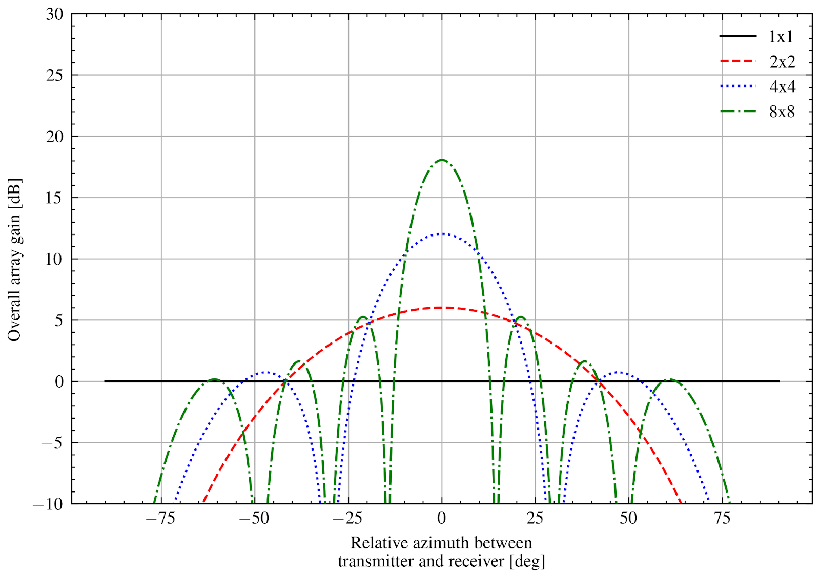
The array and beamforming gain, computed as outlined in [Rebato2018] using the
CalcBeamformingGainfunction. This term supports the presence of multiple antenna elements both at the transmitter and at the receiver and arbitrary antenna radiation patterns. Specifically, the array gain is compute as:

where:
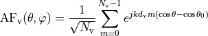
and:
In turn,  ,
,  are the number of horizontal and vertical antenna
elements respectively,
are the number of horizontal and vertical antenna
elements respectively,  ,
,  are the element spacing in the
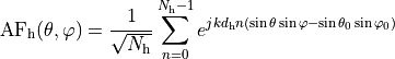
horizontal and vertical direction respectively. The figures below depict the resulting
array radiation pattern versus the relative azimuth of transmitter and receiver, for antenna
arrays featuring 3GPP TR 38.901 (
are the element spacing in the
horizontal and vertical direction respectively. The figures below depict the resulting
array radiation pattern versus the relative azimuth of transmitter and receiver, for antenna
arrays featuring 3GPP TR 38.901 (ThreeGppAntennaModel, top) and isotropic
(IsotropicAntennaModel, bottom) antenna elements, respectively.
These figures match the corresponding plots of [Asplund].
Radiation pattern produced by the CalcBeamformingGain method when using
antenna arrays featuring ThreeGppAntennaModel antenna elements, for various
Uniform Planar Array (UPA) configurations.
Radiation pattern produced by the CalcBeamformingGain method when using
antenna arrays featuring IsotropicAntennaModel antenna elements, for various
Uniform Planar Array (UPA) configurations.
Whenever the link is in NLOS, a penalty factor is introduced, to account for beam misalignment due to the lack of a dominant multipath component [Kulkarni].
A fast fading term, sampled using the Fluctuating Two Ray (FTR) model distribution [Romero]. The latter is a fading model which is more general than typical ones, taking into account two dominant specular components and a mixture of scattered paths. As, a consequence it has been shown to provide a better fit to fading phenomena at mmWaves. The model parameters are automatically picked once the simulation scenario is set, using a lookup table which associates the simulation parameters (such as carrier frequency and LOS condition) to the FTR parameters providing the best fit to the corresponding TR 38.901 channel statistics. As a consequence, this channel model can be used for all the frequencies which are supported by the 38.901 model, i.e., 0.5-100 GHz. The calibration has been done by first obtaining the statistics of the channel gain due to the small-scale fading in the 3GPP model, using an ad hoc simulation script (
src/spectrum/examples/three-gpp-two-ray-channel-calibration.cc). Then, this information has been used as a reference to estimate the FTR parameters yielding the closest (in a goodness-of-fit sense) fading realizations, using a custom Python script (src/spectrum/utils/two-ray-to-three-gpp-ch-calibration.py).
Note:
To then obtain a full channel model characterization, the model is intended to be used in conjunction of the path loss and shadowing capability provided by the
ThreeGppPropagationLossModelclass. Indeed, the goal of this model is to provide channel realizations which are as close as possible to ones of [TR38901], but at a fraction of the complexity. Since the path loss and shadowing terms are not computationally demanding anyway, the ones of [Zugno2020] have been kept;Currently, the value of NLoS beamforming factor penalty factor is taken from the preliminary work of [Kulkarni] and it is scenario-independent; As future work, the possibility of using scenario-dependent penalty factors will be investigated.
29.4.3.3. Calibration
The purpose of the calibration procedures is to compute offline a look-up table which associates the FTR fading model parameters with the simulation parameters. In particular, the [TR38901] fading distributions depend on:
The scenario (RMa, UMa, UMi-StreetCanyon, InH-OfficeOpen, InH-OfficeMixed);
The LOS condition (LoS/NLoS); and
The carrier frequency.
As a consequence, the calibration output is a map which associates LoS condition and scenario to a list of carrier frequency-FTR parameters values. The latter represent the FTR parameters yielding channel realizations which exhibit the closest statistics to [TR38901].
The actual calibration is a two-step procedure which:
1. First generates reference channel gain curves using the
src/spectrum/examples/three-gpp-two-ray-channel-calibration.cc simulation script.
Specifically, the script samples numRealizations channel realizations and computes for each of them
the end-to-end channel gain by setting the speed of the TX and RX pair to  , disabling the shadowing
and fixing the LOS condition. In such a way, any variation around the mean is due to the small-scale fading only.
The channel gain samples are produced, and returned on output conditioned on the value of
, disabling the shadowing
and fixing the LOS condition. In such a way, any variation around the mean is due to the small-scale fading only.
The channel gain samples are produced, and returned on output conditioned on the value of
enableOutput, for each combination of LoS condition, channel model scenario and carrier frequency. The
latter cover the whole [TR38901] frequency range of 0.5 - 100 GHz with a relatively sparse resolution
(500 MHz), since the dependency of the fading distribution with respect to the carrier frequency is actually
relatively weak.
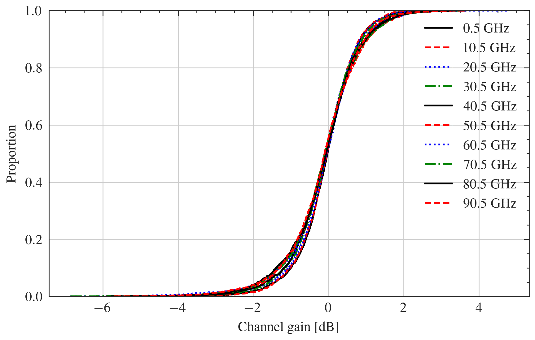
Empirical CDF of the reference channel gains obtained using the three-gpp-two-ray-channel-calibration
simulation script when keeping a fixed LoS condition and channel scenario and varying the carrier
frequency only.
2. Then, the output of the above script is parsed by the two-ray-to-three-gpp-ch-calibration.py
Python companion script. In particular, reference ECDFs are obtained from the channel gains sampled using the
model of [TR38901]. In turn, the reference ECDFs (one for each LoS condition, channel model scenario
and carrier frequency combination) are compared to FTR distributions ECDFs obtained using different values
of the parameters. Finally, the parameters which provide the best fit (in a goodness-of-fit sense) for
the specific scenario, LOS condition and carrier frequency are found. The parameters to test are picked initially
by performing an exhaustive search within a discrete grid of possible values, and then by iteratively refining
the previous search runs by scanning the neighborhood of the most recent identified values.
In such regard, the Anderson-Darling statistical test is used to rank the various FTR distributions
and eventually pick the one providing the closest approximation to the reference statistics.
29.4.3.4. Testing
The test suite TwoRaySplmTestSuite includes three test cases:
FtrFadingModelAverageTest, which checks that the average of the Fluctuating Two Ray (FTR) fading model realizations is consistent with the theoretical value provided in [Romero].ArrayResponseTest, which checks that the overall array response at boresight computed by the ùCalcBeamformingGainfunction coincides with the expected theoretical values.OverallGainAverageTest, which checks that the average overall channel gain obtained using theDoCalcRxPowerSpectralDensitymethod of theTwoRaySpectrumPropagationLossModelclass is close (it is, after all, a simplified and performance-oriented model) to the one obtained using theThreeGppSpectrumPropagationLossModelandThreeGppChannelModelclasses.
29.4.3.5. References
- Pagin2023
Pagin, Matteo, Sandra Lagen, Biljana Bojovic, Michele Polese, Michele Zorzi. 2023. “Improving the Efficiency of MIMO Simulations in ns-3” In Proceedings of the 2023 Workshop on ns-3, pp. 1–9. 2023
- Zugno2020(1,2)
Zugno, Tommaso, Michele Polese, Natale Patriciello, Biljana Bojović, Sandra Lagen, Michele Zorzi. “Implementation of a spatial channel model for ns-3.” In Proceedings of the 2020 Workshop on ns-3, pp. 49-56. 2020.
- Polese2018
Michele Polese, Michele Zorzi. “Impact of channel models on the end-to-end performance of mmwave cellular networks”. In: 2018 IEEE 19th International Workshop on Signal Processing Advances in Wireless Communications (SPAWC).
- Rebato2018
Rebato, Mattia, Laura Resteghini, Christian Mazzucco, Michele Zorzi. “Study of realistic antenna patterns in 5G mmWave cellular scenarios”. In: 2018 IEEE International Conference on Communications (ICC).
- Romero(1,2)
Romero-Jerez, Juan M., F. Javier Lopez-Martinez, José F. Paris, Andrea J. Goldsmith. “The fluctuating two-ray fading model: Statistical characterization and performance analysis”. In: IEEE Transactions on Wireless Communications 16.7 (2017).
- Kulkarni(1,2)
Kulkarni, Mandar N., Eugene Visotsky, Jeffrey G. Andrews. “Correction factor for analysis of MIMO wireless networks with highly directional beamforming.”, IEEE Wireless Communications Letters, 2018
- Asplund
Asplund, Henrik, David Astely, Peter von Butovitsch, Thomas Chapman, Mattias Frenne, Farshid Ghasemzadeh, Måns Hagström et al. Advanced Antenna Systems for 5G Network Deployments: Bridging the Gap Between Theory and Practice. Academic Press, 2020.
29.4.4. 3GPP TR 38.811 Non-Terrestrial Networks
3GPP with [3GPPTR38811] has extended the channel model presented in [3GPPTR38901] to support the so called Non-Terrestrial Networks (NTN), i.e. communication scenarios where the propagation of the signal travels through the atmosphere. The channel spectrum estimation procedure is the same as the one described in [3GPPTR38901], with a new set of parameters.
29.4.4.1. Use-cases
The use-cases for this channel model include simulations in 3D/vertical environments with communicating nodes placed in different types of orbit, in the atmosphere and/or on the ground.
29.4.4.2. Implementation
The channel spectrum estimation procedure is already implemented (as described in [ns3Zugno] ) into the classes
ThreeGppChannelModel and ThreeGppSpectrumPropagationLossModel, that have been extended to support NTN through the
introduction of the appropriate parameters.
3GPP considers two frequencies of interest: S-band (2GHz) and Ka-band (20/30GHz). Many channel parameters are dependent
on the frequency band in use, but no specific range of frequencies of these bands has been given by 3GPP. Hence, this
implementation considers S-band anything below 13GHz, and Ka-band anything above it.
Four propagation scenarios are identified, in decreasing order of building height and density: Dense Urban, Urban,
Suburban and Rural. Channel estimation parameters are scenario-dependent.
Note: For satellite, the parameters that describe the departure angle spread are 0. Thus, in the logarithmic scale
at which these parameters are represented is  .
.
29.4.4.3. References
- ns3Zugno
Zugno Tommaso, Michele Polese, Natale Patriciello, Biljana Bojović, Sandra Lagen, Michele Zorzi. “Implementation of a spatial channel model for ns-3.” In Proceedings of the 2020 Workshop on ns-3, pp. 49-56. 2020.
- 3GPPTR38901(1,2)
3GPP. 2018. TR 38.901. Study on channel for frequencies from 0.5 to 100 GHz. V.15.0.0. (2018-06).
- 3GPPTR38811
3GPP. 2018. TR 38.811, Study on New Radio (NR) to support non-terrestrial networks, V15.4.0. (2020-09).
29.4.5. Wraparound Models
The wrap around mechanism is a simulation technique used in cellular network modeling to eliminate edge effects and create a more realistic interference environment. The most common setup used by 3GPP is the hexagonal deployment wraparound, which transforms a finite hexagonal cellular cluster into what appears to be an infinite network by creating virtual copies of the cluster around the original one.
This also can significantly reduce memory and computational requirements of simulations to achieve similar results in respect to interference, avoiding the simulation of additional rings and then filtering only central rings with equivalent interference.
29.4.5.1. WraparoundModel Implementation
When a wraparound model is aggregated to the SingleModelSpectrumChannel or MultiModelSpectrumChannel,
the base class WraparoundModel creates a virtual MobilityModel for the transmitter, in respect to each
receiver.
The virtual MobilityModel is carried via the SpectrumSignalParameters to the receiver, which
must use that model to retrieve the transmitter position, NodeId and buildings related information during StartRx.
The base WraparoundModel only reuses the existing transmitter mobility model, while its children classes may
implement different wraparound techniques.
29.4.5.2. HexagonalWraparoundModel Implementation
HexagonalWraparoundModel implements wraparound for the standard cellular network setups using hexagonal clusters,
and is based on [Panwar]. Without wraparound, only the central cells experience symmetric interference from all
directions. Edge cells receive unrealistic interference patterns because they lack neighboring cells on certain sides,
making their performance data statistically invalid for real-world analysis. The wrap around mechanism addresses
this “edge effect” problem by ensuring all cells in the simulation experience equivalent interference conditions.
For this reason, wraparound is mandatory for 5G NR calibration of selected scenarios, as defined in [TR38901].
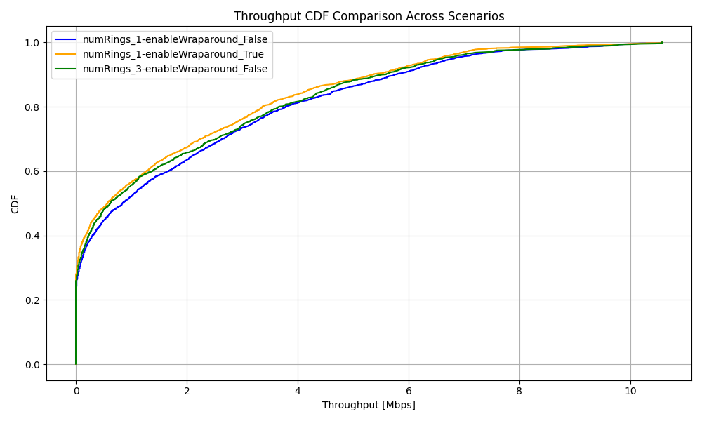
Ring 1 setup with 7 tri-sector cell clusters, with (orange) and without wraparound (blue), plus ring 3 setup with 19 tri-sector cell clusters without wraparound (green).
Interference with ring 1 and wraparound (orange) is higher than even ring 3 (green). This, in spite of only simulating 7 tri-cell clusters of ring 1 versus the 19 clusters of ring 3. The interference of both ring 1 with wraparound and ring 3 have much much higher than ring 1 without wraparound (blue). As a result, throughput without wraparound is unrealistically high (indicated by lower curves shifted to the right). This is confirmed in the following right figure.
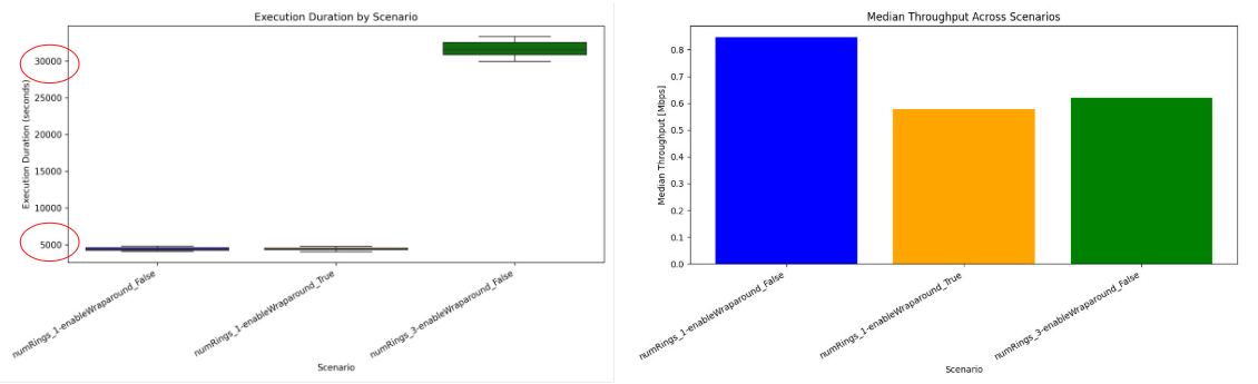
Left: Execution times of ring 1 setup with and without wraparound, plus ring 3 setup without wraparound in an AMD Ryzen Threadripper PRO 7965WX. Right: Median throughput of the different configurations.
Since the computational cost of wireless simulations scales quadratically with the number of nodes in the channel, we significantly reduce computational costs by cutting the number of simulated clusters. For this particular 5G-NR outdoor calibration example with different number of rings and wraparound, the speedup of ring 1 with wraparound against ring 3 without wraparound is of 6x, for comparable results.
Note: ring 3 simulations without wraparound require the user to manually filtering results to only cells and UEs that are part of the ring 1 cell clusters. This is because they suffer first and second tier interference. The remaining results for 12 out of 19 cells, and their respective UEs, would be discarded.
The wrap around mechanism operates by creating six additional virtual copies of the original hexagonal cluster, positioned symmetrically around the central cluster. It usually follows these steps:
Virtual Cluster Creation: Six copies of the original cluster are mathematically placed around the central cluster to simulate an infinite grid
Distance Calculation: For each signal transmission, the system calculates seven different distances - one to the actual transmitter and six to the virtual transmitter positions
Minimum Distance Selection: The shortest distance is used for path loss and signal strength calculations, ensuring realistic propagation effects
UE Mobility Handling: When a user device moves to connect with a virtual cell, it’s automatically repositioned within the central cluster while maintaining the same relative position to its serving cell (moving UE to central cluster is not currently implemented)
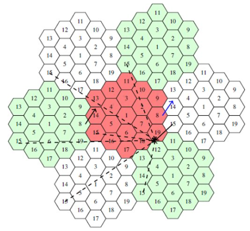
Virtual cell clusters (white and green) around real cell cluster (red). Virtual distances are shown as dashed arrows. The virtual transmitter position that results in the smallest distance to receiver is used in the virtual mobility model. [Panwar]
The technique is implemented using geometric distance calculations with specific equations for different cluster sizes: - ring 3: 19-site clusters: Standard configuration with 2-tier interference (57 cells for tri-sector antennas) - ring 1: 7-site clusters: Smaller configuration with 1-tier interference (21 cells for tri-sector antennas) - ring 0: 3-site clusters: Minimal configuration for quick testing (9 cells for tri-sector antennas)
Before start transmitting, each site position needs to be registered to the HexagonalWraparoundModel via
AddSitePosition(Vector3D position). The number of sites should also be set via SetNumSites(uint8_t sites).
Finally, the inter-site distance (ISD) must be set via SetSiteDistance(double isd_in_meters).
This can be automatically done by hexagonal deployment helpers of LTE and NR, by setting the EnableWraparound
attribute to true. After setting up the hexagonal deployment, the user should call GetWraparoundModel method
of the hexagonal deployment helper, and then aggregate that model to the spectrum channel model.
29.4.5.3. Caveats and Limitations
This implementation does not simply model edge interference in a localized or realistic way. Instead, because all signals are routed through higher-layer protocols, the effect resembles a “wormhole” model where transmissions can unrealistically appear at distant points in the topology. The transmitter itself stays fixed, but its signals may propagate as if emerging from arbitrary locations, depending on geometry and inter-site distances.
A side-effect is that mobility and handover do not strictly reflect physical adjacency. Simulations may misleadingly suggest a larger or denser deployment, allowing handover not just to neighboring cells but also to virtually adjacent ones (including cells that are physically on opposite sides of the layout). Plots can therefore be confusing: devices that look widely separated in absolute position might be treated as if they were close in virtual space.
The use of virtual mobility inside the spectrum channel models further complicates interpretation. Transmitters are treated as if they relocate, and any additional attenuation (such as building shadowing modeled through ns-3 propagation loss and buildings modules) is applied even though the device itself never actually moved. The buildings themselves are not virtualized, but buildings deployed into the non-virtualized topology still affect virtual transmissions.
[Panwar] discusses the use of wraparound for mobility models also, such that a node that left the physical site boundaries would wormhole around and reappear within the site at the mirror location. This means replacing the physical position with the virtual position when going out of physical cell areas, so the node stays within the physical topology throughout the simulation. This is not currently implemented. As such, nodes may appear outside of physical cells, but still are considered as transmitting from within the virtual cells.
29.4.5.4. References
- Panwar(1,2)
R. S. Panwar and K. M. Sivalingam, “Implementation of wrap around mechanism for system level simulation of LTE cellular networks in NS3,” 2017 IEEE 18th International Symposium on A World of Wireless, Mobile and Multimedia Networks (WoWMoM), Macau, 2017, pp. 1-9, doi: 10.1109/WoWMoM.2017.7974289