
19.2. User Documentation
19.2.1. Background
We assume the reader is already familiar with how to use the ns-3 simulator to run generic simulation programs. If this is not the case, we strongly recommend the reader to consult [ns3tutorial].
19.2.2. Usage Overview
The ns-3 LTE model is a software library that allows the simulation of LTE networks, optionally including the Evolved Packet Core (EPC). The process of performing such simulations typically involves the following steps:
Define the scenario to be simulated
Write a simulation program that recreates the desired scenario topology/architecture. This is done accessing the ns-3 LTE model library using the
ns3::LteHelperAPI defined insrc/lte/helper/lte-helper.h.Specify configuration parameters of the objects that are being used for the simulation. This can be done using input files (via the
ns3::ConfigStore) or directly within the simulation program.Configure the desired output to be produced by the simulator
Run the simulation.
All these aspects will be explained in the following sections by means of practical examples.
19.2.3. Basic simulation program
Here is the minimal simulation program that is needed to do an LTE-only simulation (without EPC).
Initial boilerplate:
#include "ns3/core-module.h"
#include "ns3/network-module.h"
#include "ns3/mobility-module.h"
#include "ns3/lte-module.h"

using namespace ns3;

int main(int argc, char *argv[])
{
  // the rest of the simulation program follows
Create an
LteHelperobject:Ptr<LteHelper> lteHelper = CreateObject<LteHelper>();
This will instantiate some common objects (e.g., the Channel object) and provide the methods to add eNBs and UEs and configure them.
Create
Nodeobjects for the eNB(s) and the UEs:NodeContainer enbNodes; enbNodes.Create(1); NodeContainer ueNodes; ueNodes.Create(2);
Note that the above Node instances at this point still don’t have an LTE protocol stack installed; they’re just empty nodes.
Configure the Mobility model for all the nodes:
MobilityHelper mobility;
mobility.SetMobilityModel("ns3::ConstantPositionMobilityModel");
mobility.Install(enbNodes);
mobility.SetMobilityModel("ns3::ConstantPositionMobilityModel");
mobility.Install(ueNodes);
The above will place all nodes at the coordinates (0,0,0). Please refer to the documentation of the ns-3 mobility model for how to set your own position or configure node movement.
Install an LTE protocol stack on the eNB(s):
NetDeviceContainer enbDevs;
enbDevs = lteHelper->InstallEnbDevice(enbNodes);
Install an LTE protocol stack on the UEs:
NetDeviceContainer ueDevs;
ueDevs = lteHelper->InstallUeDevice(ueNodes);
Attach the UEs to an eNB. This will configure each UE according to the eNB configuration, and create an RRC connection between them:
lteHelper->Attach(ueDevs, enbDevs.Get(0));
Activate a data radio bearer between each UE and the eNB it is attached to:
enum EpsBearer::Qci q = EpsBearer::GBR_CONV_VOICE;
EpsBearer bearer(q);
lteHelper->ActivateDataRadioBearer(ueDevs, bearer);
this method will also activate two saturation traffic generators for that bearer, one in uplink and one in downlink.
Set the stop time:
Simulator::Stop(Seconds(0.005));
This is needed otherwise the simulation will last forever, because (among others) the start-of-subframe event is scheduled repeatedly, and the ns-3 simulator scheduler will hence never run out of events.
Run the simulation:
Simulator::Run();
Cleanup and exit:
Simulator::Destroy();
return 0;
}
For how to compile and run simulation programs, please refer to [ns3tutorial].
19.2.4. Configuration of LTE model parameters
All the relevant LTE model parameters are managed through the ns-3 attribute system. Please refer to the [ns3tutorial] and [ns3manual] for detailed information on all the possible methods to do it (environmental variables, C++ API, GtkConfigStore…).
In the following, we just briefly summarize
how to do it using input files together with the ns-3 ConfigStore.
First of all, you need to put the following in your simulation
program, right after main () starts:
CommandLine cmd(__FILE__);
cmd.Parse(argc, argv);
ConfigStore inputConfig;
inputConfig.ConfigureDefaults();
// parse again so you can override default values from the command line
cmd.Parse(argc, argv);
for the above to work, make sure you also #include "ns3/config-store.h".
Now create a text file named (for example) input-defaults.txt
specifying the new default values that you want to use for some attributes:
default ns3::LteHelper::Scheduler "ns3::PfFfMacScheduler"
default ns3::LteHelper::PathlossModel "ns3::FriisSpectrumPropagationLossModel"
default ns3::LteEnbNetDevice::UlBandwidth "25"
default ns3::LteEnbNetDevice::DlBandwidth "25"
default ns3::LteEnbNetDevice::DlEarfcn "100"
default ns3::LteEnbNetDevice::UlEarfcn "18100"
default ns3::LteUePhy::TxPower "10"
default ns3::LteUePhy::NoiseFigure "9"
default ns3::LteEnbPhy::TxPower "30"
default ns3::LteEnbPhy::NoiseFigure "5"
Supposing your simulation program is called
src/lte/examples/lte-sim-with-input, you can now pass these
settings to the simulation program in the following way:
./ns3 run src/lte/examples/lte-sim-with-input
--command-template="%s --ns3::ConfigStore::Filename=input-defaults.txt
--ns3::ConfigStore::Mode=Load --ns3::ConfigStore::FileFormat=RawText"
Furthermore, you can generate a template input file with the following command:
./ns3 run src/lte/examples/lte-sim-with-input
--command-template="%s --ns3::ConfigStore::Filename=input-defaults.txt
--ns3::ConfigStore::Mode=Save --ns3::ConfigStore::FileFormat=RawText"
note that the above will put in the file input-defaults.txt all
the default values that are registered in your particular build of the
simulator, including lots of non-LTE attributes.
19.2.5. Configure LTE MAC Scheduler
There are several types of LTE MAC scheduler user can choose here. User can use following codes to define scheduler type:
Ptr<LteHelper> lteHelper = CreateObject<LteHelper>();
lteHelper->SetSchedulerType("ns3::FdMtFfMacScheduler");    // FD-MT scheduler
lteHelper->SetSchedulerType("ns3::TdMtFfMacScheduler");    // TD-MT scheduler
lteHelper->SetSchedulerType("ns3::TtaFfMacScheduler");     // TTA scheduler
lteHelper->SetSchedulerType("ns3::FdBetFfMacScheduler");   // FD-BET scheduler
lteHelper->SetSchedulerType("ns3::TdBetFfMacScheduler");   // TD-BET scheduler
lteHelper->SetSchedulerType("ns3::FdTbfqFfMacScheduler");  // FD-TBFQ scheduler
lteHelper->SetSchedulerType("ns3::TdTbfqFfMacScheduler");  // TD-TBFQ scheduler
lteHelper->SetSchedulerType("ns3::PssFfMacScheduler");     //PSS scheduler
TBFQ and PSS have more parameters than other schedulers. Users can define those parameters in following way:
* TBFQ scheduler::

 Ptr<LteHelper> lteHelper = CreateObject<LteHelper>();
 lteHelper->SetSchedulerAttribute("DebtLimit", IntegerValue(yourvalue)); // default value -625000 bytes(-5Mb)
 lteHelper->SetSchedulerAttribute("CreditLimit", UintegerValue(yourvalue)); // default value 625000 bytes(5Mb)
 lteHelper->SetSchedulerAttribute("TokenPoolSize", UintegerValue(yourvalue)); // default value 1 byte
 lteHelper->SetSchedulerAttribute("CreditableThreshold", UintegerValue(yourvalue)); // default value 0

* PSS scheduler::

 Ptr<LteHelper> lteHelper = CreateObject<LteHelper>();
 lteHelper->SetSchedulerAttribute("nMux", UIntegerValue(yourvalue)); // the maximum number of UE selected by TD scheduler
 lteHelper->SetSchedulerAttribute("PssFdSchedulerType", StringValue("CoItA")); // PF scheduler type in PSS
In TBFQ, default values of debt limit and credit limit are set to -5Mb and 5Mb respectively based on paper [FABokhari2009].
Current implementation does not consider credit threshold ( = 0). In PSS, if user does not define nMux,
PSS will set this value to half of total UE. The default FD scheduler is PFsch.
= 0). In PSS, if user does not define nMux,
PSS will set this value to half of total UE. The default FD scheduler is PFsch.
In addition, token generation rate in TBFQ and target bit rate in PSS need to be configured by Guarantee Bit Rate (GBR) or Maximum Bit Rate (MBR) in epc bearer QoS parameters. Users can use following codes to define GBR and MBR in both downlink and uplink:
Ptr<LteHelper> lteHelper = CreateObject<LteHelper>();
enum EpsBearer::Qci q = EpsBearer::yourvalue;  // define Qci type
GbrQosInformation qos;
qos.gbrDl = yourvalue; // Downlink GBR
qos.gbrUl = yourvalue; // Uplink GBR
qos.mbrDl = yourvalue; // Downlink MBR
qos.mbrUl = yourvalue; // Uplink MBR
EpsBearer bearer(q, qos);
lteHelper->ActivateDedicatedEpsBearer(ueDevs, bearer, EpcTft::Default());
In PSS, TBR is obtained from GBR in bearer level QoS parameters. In TBFQ, token generation rate is obtained from the MBR setting in bearer level QoS parameters, which therefore needs to be configured consistently. For constant bit rate (CBR) traffic, it is suggested to set MBR to GBR. For variance bit rate (VBR) traffic, it is suggested to set MBR k times larger than GBR in order to cover the peak traffic rate. In current implementation, k is set to three based on paper [FABokhari2009]. In addition, current version of TBFQ does not consider RLC header and PDCP header length in MBR and GBR. Another parameter in TBFQ is packet arrival rate. This parameter is calculated within scheduler and equals to the past average throughput which is used in PF scheduler.
Many useful attributes of the LTE-EPC model will be described in the
following subsections. Still, there are many attributes which are not
explicitly mentioned in the design or user documentation, but which
are clearly documented using the ns-3 attribute system. You can easily
print a list of the attributes of a given object together with their
description and default value passing --PrintAttributes= to a simulation
program, like this:
./ns3 run lena-simple --command-template="%s --PrintAttributes=ns3::LteHelper"
You can try also with other LTE and EPC objects, like this:
./ns3 run lena-simple --command-template="%s --PrintAttributes=ns3::LteEnbNetDevice"
./ns3 run lena-simple --command-template="%s --PrintAttributes=ns3::LteEnbMac"
./ns3 run lena-simple --command-template="%s --PrintAttributes=ns3::LteEnbPhy"
./ns3 run lena-simple --command-template="%s --PrintAttributes=ns3::LteUePhy"
./ns3 run lena-simple --command-template="%s --PrintAttributes=ns3::PointToPointEpcHelper"
19.2.6. Simulation Output
The ns-3 LTE model currently supports the output to file of PHY, MAC, RLC and PDCP level Key Performance Indicators (KPIs). You can enable it in the following way:
Ptr<LteHelper> lteHelper = CreateObject<LteHelper>();

// configure all the simulation scenario here...

lteHelper->EnablePhyTraces();
lteHelper->EnableMacTraces();
lteHelper->EnableRlcTraces();
lteHelper->EnablePdcpTraces();

Simulator::Run();
RLC and PDCP KPIs are calculated over a time interval and stored on ASCII
files, two for RLC KPIs and two for PDCP KPIs, in each case one for
uplink and one for downlink. The time interval duration can be controlled using the attribute
ns3::RadioBearerStatsCalculator::EpochDuration.
The columns of the RLC KPI files is the following (the same for uplink and downlink):
start time of measurement interval in seconds since the start of simulation
end time of measurement interval in seconds since the start of simulation
Cell ID
unique UE ID (IMSI)
cell-specific UE ID (RNTI)
Logical Channel ID
Number of transmitted RLC PDUs
Total bytes transmitted.
Number of received RLC PDUs
Total bytes received
Average RLC PDU delay in seconds
Standard deviation of the RLC PDU delay
Minimum value of the RLC PDU delay
Maximum value of the RLC PDU delay
Average RLC PDU size, in bytes
Standard deviation of the RLC PDU size
Minimum RLC PDU size
Maximum RLC PDU size
Similarly, the columns of the PDCP KPI files is the following (again, the same for uplink and downlink):
start time of measurement interval in seconds since the start of simulation
end time of measurement interval in seconds since the start of simulation
Cell ID
unique UE ID (IMSI)
cell-specific UE ID (RNTI)
Logical Channel ID
Number of transmitted PDCP PDUs
Total bytes transmitted.
Number of received PDCP PDUs
Total bytes received
Average PDCP PDU delay in seconds
Standard deviation of the PDCP PDU delay
Minimum value of the PDCP PDU delay
Maximum value of the PDCP PDU delay
Average PDCP PDU size, in bytes
Standard deviation of the PDCP PDU size
Minimum PDCP PDU size
Maximum PDCP PDU size
Note: The PDCP traces for data radio bearers are not generated when SM RLC is used.
MAC KPIs are basically a trace of the resource allocation reported by the scheduler upon the start of every subframe. They are stored in ASCII files. For downlink MAC KPIs the format is the following:
Simulation time in seconds at which the allocation is indicated by the scheduler
Cell ID
unique UE ID (IMSI)
Frame number
Subframe number
cell-specific UE ID (RNTI)
MCS of TB 1
size of TB 1
MCS of TB 2 (0 if not present)
size of TB 2 (0 if not present)
while for uplink MAC KPIs the format is:
Simulation time in seconds at which the allocation is indicated by the scheduler
Cell ID
unique UE ID (IMSI)
Frame number
Subframe number
cell-specific UE ID (RNTI)
MCS of TB
size of TB
The names of the files used for MAC KPI output can be customized via
the ns-3 attributes ns3::MacStatsCalculator::DlOutputFilename and
ns3::MacStatsCalculator::UlOutputFilename.
PHY KPIs are distributed in seven different files, configurable through the attributes
ns3::PhyStatsCalculator::DlRsrpSinrFilename
ns3::PhyStatsCalculator::UeSinrFilename
ns3::PhyStatsCalculator::InterferenceFilename
ns3::PhyStatsCalculator::DlTxOutputFilename
ns3::PhyStatsCalculator::UlTxOutputFilename
ns3::PhyStatsCalculator::DlRxOutputFilename
ns3::PhyStatsCalculator::UlRxOutputFilename
In the RSRP/SINR file, the following content is available:
Simulation time in seconds at which the allocation is indicated by the scheduler
Cell ID
unique UE ID (IMSI)
RSRP
Linear average over all RBs of the downlink SINR in linear units
The contents in the UE SINR file are:
Simulation time in seconds at which the allocation is indicated by the scheduler
Cell ID
unique UE ID (IMSI)
uplink SINR in linear units for the UE
In the interference filename the content is:
Simulation time in seconds at which the allocation is indicated by the scheduler
Cell ID
List of interference values per RB
In UL and DL transmission files the parameters included are:
Simulation time in milliseconds
Cell ID
unique UE ID (IMSI)
RNTI
Layer of transmission
MCS
size of the TB
Redundancy version
New Data Indicator flag
And finally, in UL and DL reception files the parameters included are:
Simulation time in milliseconds
Cell ID
unique UE ID (IMSI)
RNTI
Transmission Mode
Layer of transmission
MCS
size of the TB
Redundancy version
New Data Indicator flag
Correctness in the reception of the TB
Note: The traces generated by simulating the scenarios involving the RLF will have a discontinuity in time from the moment of the RLF event until the UE connects again to an eNB.
19.2.7. Fading Trace Usage
In this section we will describe how to use fading traces within LTE simulations.
19.2.7.1. Fading Traces Generation
It is possible to generate fading traces by using a dedicated matlab script provided with the code (/lte/model/fading-traces/fading-trace-generator.m). This script already includes the typical taps configurations for three 3GPP scenarios (i.e., pedestrian, vehicular and urban as defined in Annex B.2 of [TS36104]); however users can also introduce their specific configurations. The list of the configurable parameters is provided in the following:
fc: the frequency in use (it affects the computation of the doppler speed).
v_km_h: the speed of the users
traceDuration: the duration in seconds of the total length of the trace.
numRBs: the number of the resource block to be evaluated.
tag: the tag to be applied to the file generated.
The file generated contains ASCII-formatted real values organized in a matrix fashion: every row corresponds to a different RB, and every column correspond to a different temporal fading trace sample.
It has to be noted that the ns-3 LTE module is able to work with any fading trace file that complies with the above described ASCII format. Hence, other external tools can be used to generate custom fading traces, such as for example other simulators or experimental devices.
19.2.7.2. Fading Traces Usage
When using a fading trace, it is of paramount importance to specify correctly the trace parameters in the simulation, so that the fading model can load and use it correctly. The parameters to be configured are:
TraceFilename: the name of the trace to be loaded (absolute path, or relative path w.r.t. the path from where the simulation program is executed);
TraceLength: the trace duration in seconds;
SamplesNum: the number of samples;
WindowSize: the size of the fading sampling window in seconds;
It is important to highlight that the sampling interval of the fading trace has to be 1 ms or greater, and in the latter case it has to be an integer multiple of 1 ms in order to be correctly processed by the fading module.
The default configuration of the matlab script provides a trace 10 seconds long, made of 10,000 samples (i.e., 1 sample per TTI=1ms) and used with a windows size of 0.5 seconds amplitude. These are also the default values of the parameters above used in the simulator; therefore their settage can be avoided in case the fading trace respects them.
In order to activate the fading module (which is not active by default) the following code should be included in the simulation program:
Ptr<LteHelper> lteHelper = CreateObject<LteHelper>();
lteHelper->SetFadingModel("ns3::TraceFadingLossModel");
And for setting the parameters:
lteHelper->SetFadingModelAttribute("TraceFilename", StringValue("src/lte/model/fading-traces/fading_trace_EPA_3kmph.fad"));
lteHelper->SetFadingModelAttribute("TraceLength", TimeValue(Seconds(10)));
lteHelper->SetFadingModelAttribute("SamplesNum", UintegerValue(10000));
lteHelper->SetFadingModelAttribute("WindowSize", TimeValue(Seconds(0.5)));
lteHelper->SetFadingModelAttribute("RbNum", UintegerValue(100));
It has to be noted that, TraceFilename does not have a default value, therefore is has to be always set explicitly.
The simulator provide natively three fading traces generated according to the configurations defined in in Annex B.2 of [TS36104]. These traces are available in the folder src/lte/model/fading-traces/). An excerpt from these traces is represented in the following figures.
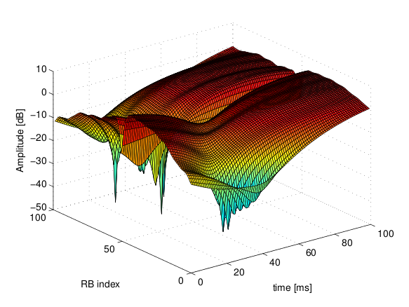
Excerpt of the fading trace included in the simulator for a pedestrian scenario (speed of 3 kmph).
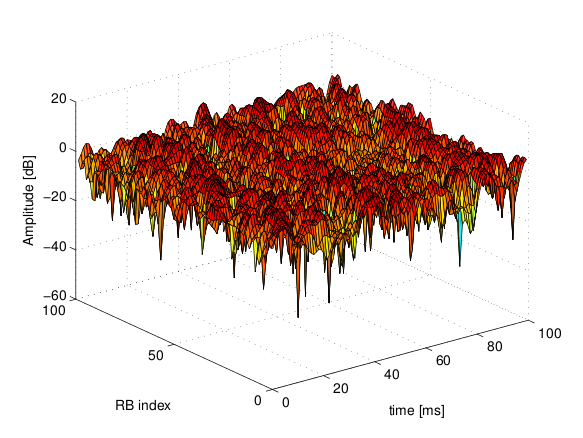
Excerpt of the fading trace included in the simulator for a vehicular scenario (speed of 60 kmph).
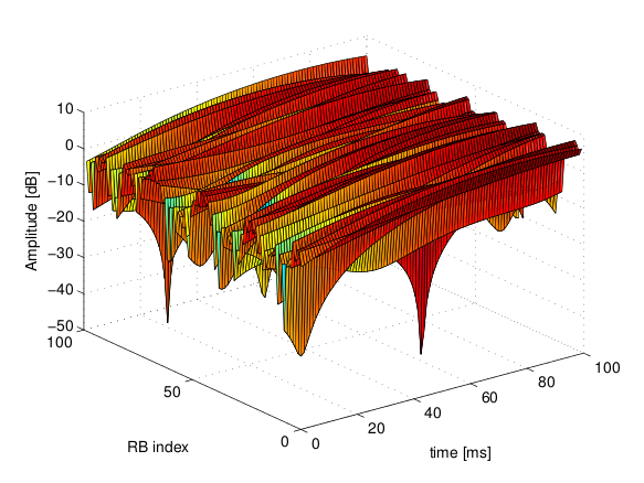
Excerpt of the fading trace included in the simulator for an urban scenario (speed of 3 kmph).
19.2.8. Mobility Model with Buildings
We now explain by examples how to use the buildings model (in particular, the MobilityBuildingInfo and the BuildingPropagationModel classes) in an ns-3 simulation program to setup an LTE simulation scenario that includes buildings and indoor nodes.
Header files to be included:
#include "ns3/mobility-building-info.h"
#include "ns3/buildings-propagation-loss-model.h"
#include "ns3/building.h"
Pathloss model selection:
Ptr<LteHelper> lteHelper = CreateObject<LteHelper>();

lteHelper->SetAttribute("PathlossModel", StringValue("ns3::BuildingsPropagationLossModel"));
EUTRA Band Selection
The selection of the working frequency of the propagation model has to be done with the standard ns-3 attribute system as described in the correspond section (“Configuration of LTE model parameters”) by means of the DlEarfcn and UlEarfcn parameters, for instance:
lteHelper->SetEnbDeviceAttribute("DlEarfcn", UintegerValue(100));
lteHelper->SetEnbDeviceAttribute("UlEarfcn", UintegerValue(18100));
It is to be noted that using other means to configure the frequency used by the propagation model (i.e., configuring the corresponding BuildingsPropagationLossModel attributes directly) might generates conflicts in the frequencies definition in the modules during the simulation, and is therefore not advised.
Mobility model selection:
MobilityHelper mobility;
mobility.SetMobilityModel("ns3::ConstantPositionMobilityModel");

It is to be noted that any mobility model can be used.
Building creation:
double x_min = 0.0;
double x_max = 10.0;
double y_min = 0.0;
double y_max = 20.0;
double z_min = 0.0;
double z_max = 10.0;
Ptr<Building> b = CreateObject<Building>();
b->SetBoundaries(Box(x_min, x_max, y_min, y_max, z_min, z_max));
b->SetBuildingType(Building::Residential);
b->SetExtWallsType(Building::ConcreteWithWindows);
b->SetNFloors(3);
b->SetNRoomsX(3);
b->SetNRoomsY(2);
This will instantiate a residential building with base of 10 x 20 meters and height of 10 meters whose external walls are of concrete with windows; the building has three floors and has an internal 3 x 2 grid of rooms of equal size.
Node creation and positioning:
ueNodes.Create(2);
mobility.Install(ueNodes);
BuildingsHelper::Install(ueNodes);
NetDeviceContainer ueDevs;
ueDevs = lteHelper->InstallUeDevice(ueNodes);
Ptr<ConstantPositionMobilityModel> mm0 = enbNodes.Get(0)->GetObject<ConstantPositionMobilityModel>();
Ptr<ConstantPositionMobilityModel> mm1 = enbNodes.Get(1)->GetObject<ConstantPositionMobilityModel>();
mm0->SetPosition(Vector(5.0, 5.0, 1.5));
mm1->SetPosition(Vector(30.0, 40.0, 1.5));
Finalize the building and mobility model configuration:
BuildingsHelper::MakeMobilityModelConsistent();
See the documentation of the buildings module for more detailed information.
19.2.9. PHY Error Model
The Physical error model consists of the data error model and the downlink control error model, both of them active by default. It is possible to deactivate them with the ns3 attribute system, in detail:
Config::SetDefault("ns3::LteSpectrumPhy::CtrlErrorModelEnabled", BooleanValue(false));
Config::SetDefault("ns3::LteSpectrumPhy::DataErrorModelEnabled", BooleanValue(false));
19.2.10. MIMO Model
Is this subsection we illustrate how to configure the MIMO parameters. LTE defines 7 types of transmission modes:
Transmission Mode 1: SISO.
Transmission Mode 2: MIMO Tx Diversity.
Transmission Mode 3: MIMO Spatial Multiplexity Open Loop.
Transmission Mode 4: MIMO Spatial Multiplexity Closed Loop.
Transmission Mode 5: MIMO Multi-User.
Transmission Mode 6: Closer loop single layer precoding.
Transmission Mode 7: Single antenna port 5.
According to model implemented, the simulator includes the first three transmission modes types. The default one is the Transmission Mode 1 (SISO). In order to change the default Transmission Mode to be used, the attribute DefaultTransmissionMode of the LteEnbRrc can be used, as shown in the following:
Config::SetDefault("ns3::LteEnbRrc::DefaultTransmissionMode", UintegerValue(0)); // SISO
Config::SetDefault("ns3::LteEnbRrc::DefaultTransmissionMode", UintegerValue(1)); // MIMO Tx diversity(1 layer)
Config::SetDefault("ns3::LteEnbRrc::DefaultTransmissionMode", UintegerValue(2)); // MIMO Spatial Multiplexity(2 layers)
For changing the transmission mode of a certain user during the simulation a specific interface has been implemented in both standard schedulers:
void TransmissionModeConfigurationUpdate(uint16_t rnti, uint8_t txMode);
This method can be used both for developing transmission mode decision engine (i.e., for optimizing the transmission mode according to channel condition and/or user’s requirements) and for manual switching from simulation script. In the latter case, the switching can be done as shown in the following:
Ptr<LteEnbNetDevice> lteEnbDev = enbDevs.Get(0)->GetObject<LteEnbNetDevice>();
PointerValue ptrval;
enbNetDev->GetAttribute("FfMacScheduler", ptrval);
Ptr<RrFfMacScheduler> rrsched = ptrval.Get<RrFfMacScheduler>();
Simulator::Schedule(Seconds(0.2), &RrFfMacScheduler::TransmissionModeConfigurationUpdate, rrsched, rnti, 1);
Finally, the model implemented can be reconfigured according to different MIMO models by updating the gain values (the only constraints is that the gain has to be constant during simulation run-time and common for the layers). The gain of each Transmission Mode can be changed according to the standard ns3 attribute system, where the attributes are: TxMode1Gain, TxMode2Gain, TxMode3Gain, TxMode4Gain, TxMode5Gain, TxMode6Gain and TxMode7Gain. By default only TxMode1Gain, TxMode2Gain and TxMode3Gain have a meaningful value, that are the ones derived by _[CatreuxMIMO] (i.e., respectively 0.0, 4.2 and -2.8 dB).
19.2.11. Use of AntennaModel
We now show how associate a particular AntennaModel with an eNB device
in order to model a sector of a macro eNB. For this purpose, it is
convenient to use the CosineAntennaModel provided by the ns-3
antenna module. The configuration of the eNB is to be done via the
LteHelper instance right before the creation of the
EnbNetDevice, as shown in the following:
lteHelper->SetEnbAntennaModelType("ns3::CosineAntennaModel");
lteHelper->SetEnbAntennaModelAttribute("Orientation", DoubleValue(0));
lteHelper->SetEnbAntennaModelAttribute("Beamwidth",   DoubleValue(60));
lteHelper->SetEnbAntennaModelAttribute("MaxGain",     DoubleValue(0.0));
the above code will generate an antenna model with a 60 degrees
beamwidth pointing along the X axis. The orientation is measured
in degrees from the X axis, e.g., an orientation of 90 would point
along the Y axis, and an orientation of -90 would point in the
negative direction along the Y axis. The beamwidth is the -3 dB
beamwidth, e.g, for a 60 degree beamwidth the antenna gain at an angle
of  degrees from the direction of orientation is -3 dB.
To create a multi-sector site, you need to create different ns-3 nodes
placed at the same position, and to configure separate EnbNetDevice
with different antenna orientations to be installed on each node.
19.2.12. Radio Environment Maps
By using the class RadioEnvironmentMapHelper it is possible to output
to a file a Radio Environment Map (REM), i.e., a uniform 2D grid of values
that represent the Signal-to-noise ratio in the downlink with respect
to the eNB that has the strongest signal at each point. It is possible
to specify if REM should be generated for data or control channel. Also user
can set the RbId, for which REM will be generated. Default RbId is -1, what
means that REM will generated with averaged Signal-to-noise ratio from all RBs.
To do this, you just need to add the following code to your simulation program towards the end, right before the call to Simulator::Run():
Ptr<RadioEnvironmentMapHelper> remHelper = CreateObject<RadioEnvironmentMapHelper>();
remHelper->SetAttribute("Channel", PointerValue(lteHelper->GetDownlinkSpectrumChannel()));
remHelper->SetAttribute("OutputFile", StringValue("rem.out"));
remHelper->SetAttribute("XMin", DoubleValue(-400.0));
remHelper->SetAttribute("XMax", DoubleValue(400.0));
remHelper->SetAttribute("XRes", UintegerValue(100));
remHelper->SetAttribute("YMin", DoubleValue(-300.0));
remHelper->SetAttribute("YMax", DoubleValue(300.0));
remHelper->SetAttribute("YRes", UintegerValue(75));
remHelper->SetAttribute("Z", DoubleValue(0.0));
remHelper->SetAttribute("UseDataChannel", BooleanValue(true));
remHelper->SetAttribute("RbId", IntegerValue(10));
remHelper->Install();
By configuring the attributes of the RadioEnvironmentMapHelper object
as shown above, you can tune the parameters of the REM to be
generated. Note that each RadioEnvironmentMapHelper instance can
generate only one REM; if you want to generate more REMs, you need to
create one separate instance for each REM.
Note that the REM generation is very demanding, in particular:
the run-time memory consumption is approximately 5KB per pixel. For example, a REM with a resolution of 500x500 would need about 1.25 GB of memory, and a resolution of 1000x1000 would need needs about 5 GB (too much for a regular PC at the time of this writing). To overcome this issue, the REM is generated at successive steps, with each step evaluating at most a number of pixels determined by the value of the the attribute
RadioEnvironmentMapHelper::MaxPointsPerIteration.if you generate a REM at the beginning of a simulation, it will slow down the execution of the rest of the simulation. If you want to generate a REM for a program and also use the same program to get simulation result, it is recommended to add a command-line switch that allows to either generate the REM or run the complete simulation. For this purpose, note that there is an attribute
RadioEnvironmentMapHelper::StopWhenDone(default: true) that will force the simulation to stop right after the REM has been generated.
The REM is stored in an ASCII file in the following format:
column 1 is the x coordinate
column 2 is the y coordinate
column 3 is the z coordinate
column 4 is the SINR in linear units
A minimal gnuplot script that allows you to plot the REM is given below:
set view map;
set xlabel "X"
set ylabel "Y"
set cblabel "SINR (dB)"
unset key
plot "rem.out" using ($1):($2):(10*log10($4)) with image
As an example, here is the REM that can be obtained with the example program lena-dual-stripe, which shows a three-sector LTE macrocell in a co-channel deployment with some residential femtocells randomly deployed in two blocks of apartments.
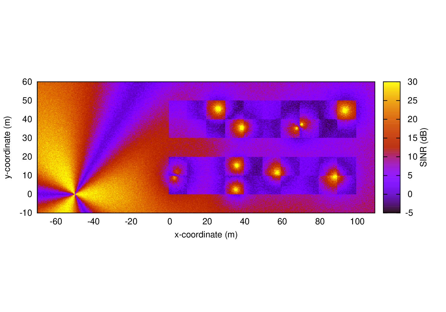
REM obtained from the lena-dual-stripe example
Note that the lena-dual-stripe example program also generate
gnuplot-compatible output files containing information about the
positions of the UE and eNB nodes as well as of the buildings,
respectively in the files ues.txt, enbs.txt and
buildings.txt. These can be easily included when using
gnuplot. For example, assuming that your gnuplot script (e.g., the
minimal gnuplot script described above) is saved in a file named
my_plot_script, running the following command would plot the
location of UEs, eNBs and buildings on top of the REM:
gnuplot -p enbs.txt ues.txt buildings.txt my_plot_script
19.2.13. AMC Model and CQI Calculation
The simulator provides two possible schemes for what concerns the selection of the MCSs and correspondingly the generation of the CQIs. The first one is based on the GSoC module [Piro2011] and works per RB basis. This model can be activated with the ns3 attribute system, as presented in the following:
Config::SetDefault("ns3::LteAmc::AmcModel", EnumValue(LteAmc::PiroEW2010));
While, the solution based on the physical error model can be controlled with:
Config::SetDefault("ns3::LteAmc::AmcModel", EnumValue(LteAmc::MiErrorModel));
Finally, the required efficiency of the PiroEW2010 AMC module can be tuned thanks to the Ber attribute(), for instance:
Config::SetDefault("ns3::LteAmc::Ber", DoubleValue(0.00005));
19.2.14. Evolved Packet Core (EPC)
We now explain how to write a simulation program that allows to simulate the EPC in addition to the LTE radio access network. The use of EPC allows to use IPv4 and IPv6 networking with LTE devices. In other words, you will be able to use the regular ns-3 applications and sockets over IPv4 and IPv6 over LTE, and also to connect an LTE network to any other IPv4 and IPv6 network you might have in your simulation.
First of all, in addition to LteHelper that we already introduced
in Basic simulation program, you need to use an additional
EpcHelper class, which will take care of creating the EPC entities and
network topology. Note that you can’t use EpcHelper directly, as
it is an abstract base class; instead, you need to use one of its
child classes, which provide different EPC topology implementations. In
this example we will consider PointToPointEpcHelper, which
implements an EPC based on point-to-point links. To use it, you need
first to insert this code in your simulation program:
Ptr<LteHelper> lteHelper = CreateObject<LteHelper>();
Ptr<PointToPointEpcHelper> epcHelper = CreateObject<PointToPointEpcHelper>();
Then, you need to tell the LTE helper that the EPC will be used:
lteHelper->SetEpcHelper(epcHelper);
the above step is necessary so that the LTE helper will trigger the appropriate EPC configuration in correspondence with some important configuration, such as when a new eNB or UE is added to the simulation, or an EPS bearer is created. The EPC helper will automatically take care of the necessary setup, such as S1 link creation and S1 bearer setup. All this will be done without the intervention of the user.
Calling lteHelper->SetEpcHelper(epcHelper) enables the use of
EPC, and has the side effect that any new LteEnbRrc that is
created will have the EpsBearerToRlcMapping attribute set to
RLC_UM_ALWAYS instead of RLC_SM_ALWAYS if the latter was
the default; otherwise, the attribute won’t be changed (e.g., if
you changed the default to RLC_AM_ALWAYS, it won’t be touched).
It is to be noted that the EpcHelper will also automatically
create the PGW node and configure it so that it can properly handle
traffic from/to the LTE radio access network. Still,
you need to add some explicit code to connect the PGW to other
IPv4/IPv6 networks (e.g., the internet, another EPC). Here is a very
simple example about how to connect a single remote host (IPv4 type)
to the PGW via a point-to-point link:
Ptr<Node> pgw = epcHelper->GetPgwNode();

// Create a single RemoteHost
NodeContainer remoteHostContainer;
remoteHostContainer.Create(1);
Ptr<Node> remoteHost = remoteHostContainer.Get(0);
InternetStackHelper internet;
internet.Install(remoteHostContainer);

// Create the internet
PointToPointHelper p2ph;
p2ph.SetDeviceAttribute("DataRate", DataRateValue(DataRate("100Gb/s")));
p2ph.SetDeviceAttribute("Mtu", UintegerValue(1500));
p2ph.SetChannelAttribute("Delay", TimeValue(Seconds(0.010)));
NetDeviceContainer internetDevices = p2ph.Install(pgw, remoteHost);
Ipv4AddressHelper ipv4h;
ipv4h.SetBase("1.0.0.0", "255.0.0.0");
Ipv4InterfaceContainer internetIpIfaces = ipv4h.Assign(internetDevices);
// interface 0 is localhost, 1 is the p2p device
Ipv4Address remoteHostAddr = internetIpIfaces.GetAddress(1);


Ipv4StaticRoutingHelper ipv4RoutingHelper;
Ptr<Ipv4StaticRouting> remoteHostStaticRouting;
remoteHostStaticRouting = ipv4RoutingHelper.GetStaticRouting(remoteHost->GetObject<Ipv4>());
remoteHostStaticRouting->AddNetworkRouteTo(epcHelper->GetEpcIpv4NetworkAddress(),
                                           Ipv4Mask("255.255.0.0"), 1);
Now, you should go on and create LTE eNBs and UEs as explained in the previous sections. You can of course configure other LTE aspects such as pathloss and fading models. Right after you created the UEs, you should also configure them for IP networking. This is done as follows. We assume you have a container for UE and eNodeB nodes like this:
NodeContainer ueNodes;
NodeContainer enbNodes;
to configure an LTE-only simulation, you would then normally do something like this:
NetDeviceContainer ueLteDevs = lteHelper->InstallUeDevice(ueNodes);
lteHelper->Attach(ueLteDevs, enbLteDevs.Get(0));
in order to configure the UEs for IP networking, you just need to additionally do like this:
// we install the IP stack on the UEs
InternetStackHelper internet;
internet.Install(ueNodes);

// assign IP address to UEs
for (uint32_t u = 0; u < ueNodes.GetN(); ++u)
  {
    Ptr<Node> ue = ueNodes.Get(u);
    Ptr<NetDevice> ueLteDevice = ueLteDevs.Get(u);
    Ipv4InterfaceContainer ueIpIface;
    ueIpIface = epcHelper->AssignUeIpv4Address(NetDeviceContainer(ueLteDevice));
    // set the default gateway for the UE
    Ptr<Ipv4StaticRouting> ueStaticRouting;
    ueStaticRouting = ipv4RoutingHelper.GetStaticRouting(ue->GetObject<Ipv4>());
    ueStaticRouting->SetDefaultRoute(epcHelper->GetUeDefaultGatewayAddress(), 1);
  }
The activation of bearers is done in a slightly different way with
respect to what done for an LTE-only simulation. First, the method
ActivateDataRadioBearer is not to be used when the EPC is
used. Second, when EPC is used, the default EPS bearer will be
activated automatically when you call LteHelper::Attach(). Third, if
you want to setup dedicated EPS bearer, you can do so using the method
LteHelper::ActivateDedicatedEpsBearer(). This method takes as a
parameter the Traffic Flow Template(TFT), which is a struct that
identifies the type of traffic that will be mapped to the dedicated
EPS bearer. Here is an example for how to setup a dedicated bearer
for an application at the UE communicating on port 1234:
Ptr<EpcTft> tft = Create<EpcTft>();
EpcTft::PacketFilter pf;
pf.localPortStart = 1234;
pf.localPortEnd = 1234;
tft->Add(pf);
lteHelper->ActivateDedicatedEpsBearer(ueLteDevs,
                                      EpsBearer(EpsBearer::NGBR_VIDEO_TCP_DEFAULT),
                                      tft);
you can of course use custom EpsBearer and EpcTft configurations, please refer to the doxygen documentation for how to do it.
Finally, you can install applications on the LTE UE nodes that communicate with remote applications over the internet. This is done following the usual ns-3 procedures. Following our simple example with a single remoteHost, here is how to setup downlink communication, with an UdpClient application on the remote host, and a PacketSink on the LTE UE (using the same variable names of the previous code snippets)
uint16_t dlPort = 1234;
PacketSinkHelper packetSinkHelper("ns3::UdpSocketFactory",
                                  InetSocketAddress(Ipv4Address::GetAny(), dlPort));
ApplicationContainer serverApps = packetSinkHelper.Install(ue);
serverApps.Start(Seconds(0.01));
UdpClientHelper client(ueIpIface.GetAddress(0), dlPort);
ApplicationContainer clientApps = client.Install(remoteHost);
clientApps.Start(Seconds(0.01));
That’s all! You can now start your simulation as usual:
Simulator::Stop(Seconds(10));
Simulator::Run();
19.2.15. Using the EPC with emulation mode
In the previous section we used PointToPoint links for the connection between the eNBs and the SGW (S1-U interface) and among eNBs (X2-U and X2-C interfaces). The LTE module supports using emulated links instead of PointToPoint links. This is achieved by just replacing the creation of LteHelper and EpcHelper with the following code:
Ptr<LteHelper> lteHelper = CreateObject<LteHelper>();
Ptr<EmuEpcHelper>  epcHelper = CreateObject<EmuEpcHelper>();
lteHelper->SetEpcHelper(epcHelper);
epcHelper->Initialize();
The attributes ns3::EmuEpcHelper::sgwDeviceName and ns3::EmuEpcHelper::enbDeviceName are used to set the name of the devices used for transporting the S1-U, X2-U and X2-C interfaces at the SGW and eNB, respectively. We will now show how this is done in an example where we execute the example program lena-simple-epc-emu using two virtual ethernet interfaces.
First of all we build ns-3 appropriately:
# configure
./ns3 configure --enable-sudo --enable-modules=lte,fd-net-device --enable-examples

# build
./ns3
Then we setup two virtual ethernet interfaces, and start wireshark to look at the traffic going through:
# note: you need to be root

# create two paired veth devices
ip link add name veth0 type veth peer name veth1
ip link show

# enable promiscuous mode
ip link set veth0 promisc on
ip link set veth1 promisc on

# bring interfaces up
ip link set veth0 up
ip link set veth1 up

# start wireshark and capture on veth0
wireshark &
We can now run the example program with the simulated clock:
./ns3 run lena-simple-epc-emu --command="%s --ns3::EmuEpcHelper::sgwDeviceName=veth0
--ns3::EmuEpcHelper::enbDeviceName=veth1"
Using wireshark, you should see ARP resolution first, then some GTP packets exchanged both in uplink and downlink.
The default setting of the example program is 1 eNB and 1UE. You can change this via command line parameters, e.g.:
./ns3 run lena-simple-epc-emu --command="%s --ns3::EmuEpcHelper::sgwDeviceName=veth0
--ns3::EmuEpcHelper::enbDeviceName=veth1 --nEnbs=2 --nUesPerEnb=2"
To get a list of the available parameters:
./ns3 run lena-simple-epc-emu --command="%s --PrintHelp"
To run with the realtime clock: it turns out that the default debug build is too slow for realtime. Softening the real time constraints with the BestEffort mode is not a good idea: something can go wrong (e.g., ARP can fail) and, if so, you won’t get any data packets out. So you need a decent hardware and the optimized build with statically linked modules:
./ns3 configure -d optimized --enable-static --enable-modules=lte --enable-examples
--enable-sudo
Then run the example program like this:
./ns3 run lena-simple-epc-emu --command="%s --ns3::EmuEpcHelper::sgwDeviceName=veth0
--ns3::EmuEpcHelper::enbDeviceName=veth1
--SimulatorImplementationType=ns3::RealtimeSimulatorImpl
--ns3::RealtimeSimulatorImpl::SynchronizationMode=HardLimit"
note the HardLimit setting, which will cause the program to terminate if it cannot keep up with real time.
The approach described in this section can be used with any type of net device. For instance, [Baldo2014] describes how it was used to run an emulated LTE-EPC network over a real multi-layer packet-optical transport network.
19.2.16. Custom Backhaul
In the previous sections, Evolved Packet Core (EPC), we explained how to write a simulation
program using EPC with a predefined backhaul network between the RAN and the EPC. We used the
PointToPointEpcHelper. This EpcHelper creates point-to-point links between the eNBs and the SGW.
We now explain how to write a simulation program that allows the simulator user to create any kind of backhaul network in the simulation program.
First of all, in addition to LteHelper, you need to use the NoBackhaulEpcHelper class, which
implements an EPC but without connecting the eNBs with the core network. It just creates the network
elements of the core network:
Ptr<LteHelper> lteHelper = CreateObject<LteHelper>();
Ptr<NoBackhaulEpcHelper> epcHelper = CreateObject<NoBackhaulEpcHelper>();
Then, as usual, you need to tell the LTE helper that the EPC will be used:
lteHelper->SetEpcHelper(epcHelper);
Now, you should create the backhaul network. Here we create point-to-point links as it is done
by the PointToPointEpcHelper. We assume you have a container for eNB nodes like this:
NodeContainer enbNodes;
We get the SGW node:
Ptr<Node> sgw = epcHelper->GetSgwNode();
And we connect every eNB from the container with the SGW with a point-to-point link. We also assign
IPv4 addresses to the interfaces of eNB and SGW with s1uIpv4AddressHelper.Assign(sgwEnbDevices)
and finally we tell the EpcHelper that this enb has a new S1 interface with
epcHelper->AddS1Interface(enb, enbS1uAddress, sgwS1uAddress), where enbS1uAddress and
sgwS1uAddress are the IPv4 addresses of the eNB and the SGW, respectively:
Ipv4AddressHelper s1uIpv4AddressHelper;

// Create networks of the S1 interfaces
s1uIpv4AddressHelper.SetBase("10.0.0.0", "255.255.255.252");

for (uint16_t i = 0; i < enbNodes.GetN(); ++i)
  {
    Ptr<Node> enb = enbNodes.Get(i);

    // Create a point to point link between the eNB and the SGW with
    // the corresponding new NetDevices on each side
    PointToPointHelper p2ph;
    DataRate s1uLinkDataRate = DataRate("10Gb/s");
    uint16_t s1uLinkMtu = 2000;
    Time s1uLinkDelay = Time(0);
    p2ph.SetDeviceAttribute("DataRate", DataRateValue(s1uLinkDataRate));
    p2ph.SetDeviceAttribute("Mtu", UintegerValue(s1uLinkMtu));
    p2ph.SetChannelAttribute("Delay", TimeValue(s1uLinkDelay));
    NetDeviceContainer sgwEnbDevices = p2ph.Install(sgw, enb);

    Ipv4InterfaceContainer sgwEnbIpIfaces = s1uIpv4AddressHelper.Assign(sgwEnbDevices);
    s1uIpv4AddressHelper.NewNetwork();

    Ipv4Address sgwS1uAddress = sgwEnbIpIfaces.GetAddress(0);
    Ipv4Address enbS1uAddress = sgwEnbIpIfaces.GetAddress(1);

    // Create S1 interface between the SGW and the eNB
    epcHelper->AddS1Interface(enb, enbS1uAddress, sgwS1uAddress);
  }
This is just an example how to create a custom backhaul network. In this other example, we connect all eNBs and the SGW to the same CSMA network:
// Create networks of the S1 interfaces
s1uIpv4AddressHelper.SetBase("10.0.0.0", "255.255.255.0");

NodeContainer sgwEnbNodes;
sgwEnbNodes.Add(sgw);
sgwEnbNodes.Add(enbNodes);

CsmaHelper csmah;
NetDeviceContainer sgwEnbDevices = csmah.Install(sgwEnbNodes);
Ptr<NetDevice> sgwDev = sgwEnbDevices.Get(0);

Ipv4InterfaceContainer sgwEnbIpIfaces = s1uIpv4AddressHelper.Assign(sgwEnbDevices);
Ipv4Address sgwS1uAddress = sgwEnbIpIfaces.GetAddress(0);

for (uint16_t i = 0; i < enbNodes.GetN(); ++i)
  {
    Ptr<Node> enb = enbNodes.Get(i);
    Ipv4Address enbS1uAddress = sgwEnbIpIfaces.GetAddress(i + 1);

    // Create S1 interface between the SGW and the eNB
    epcHelper->AddS1Interface(enb, enbS1uAddress, sgwS1uAddress);
  }
As you can see, apart from how you create the backhaul network, i.e. the point-to-point links or
the CSMA network, the important point is to tell the EpcHelper that an eNB has a new S1 interface.
Now, you should continue configuring your simulation program as it is explained in Evolved Packet Core (EPC) subsection. This configuration includes: the internet, installing the LTE eNBs and possibly configuring other LTE aspects, installing the LTE UEs and configuring them as IP nodes, activation of the dedicated EPS bearers and installing applications on the LTE UEs and on the remote hosts.
19.2.17. Network Attachment
As shown in the basic example in section Basic simulation program,
attaching a UE to an eNodeB is done by calling LteHelper::Attach function.
There are 2 possible ways of network attachment. The first method is the “manual” one, while the second one has a more “automatic” sense on it. Each of them will be covered in this section.
19.2.17.1. Manual attachment
This method uses the LteHelper::Attach function mentioned above. It has been
the only available network attachment method in earlier versions of LTE module.
It is typically invoked before the simulation begins:
lteHelper->Attach(ueDevs, enbDev); // attach one or more UEs to a single eNodeB
LteHelper::InstallEnbDevice and LteHelper::InstallUeDevice functions
must have been called before attaching. In an EPC-enabled simulation, it is also
required to have IPv4/IPv6 properly pre-installed in the UE.
This method is very simple, but requires you to know exactly which UE belongs to to which eNodeB before the simulation begins. This can be difficult when the UE initial position is randomly determined by the simulation script.
One may choose the distance between the UE and the eNodeB as a criterion for selecting the appropriate cell. It is quite simple (at least from the simulator’s point of view) and sometimes practical. But it is important to note that sometimes distance does not make a single correct criterion. For instance, the eNodeB antenna directivity should be considered as well. Besides that, one should also take into account the channel condition, which might be fluctuating if there is fading or shadowing in effect. In these kind of cases, network attachment should not be based on distance alone.
In real life, UE will automatically evaluate certain criteria and select the
best cell to attach to, without manual intervention from the user. Obviously
this is not the case in this LteHelper::Attach function. The other network
attachment method uses more “automatic” approach to network attachment, as
will be described next.
19.2.17.2. Automatic attachment using Idle mode cell selection procedure
The strength of the received signal is the standard criterion used for selecting
the best cell to attach to. The use of this criterion is implemented in the
initial cell selection process, which can be invoked by calling another
version of the LteHelper::Attach function, as shown below:
lteHelper->Attach(ueDevs); // attach one or more UEs to a strongest cell
The difference with the manual method is that the destination eNodeB is not specified. The procedure will find the best cell for the UEs, based on several criteria, including the strength of the received signal (RSRP).
After the method is called, the UE will spend some time to measure the neighbouring cells, and then attempt to attach to the best one. More details can be found in section Initial Cell Selection of the Design Documentation.
It is important to note that this method only works in EPC-enabled simulations. LTE-only simulations must resort to manual attachment method.
19.2.17.3. Closed Subscriber Group
An interesting use case of the initial cell selection process is to setup a simulation environment with Closed Subscriber Group (CSG).
For example, a certain eNodeB, typically a smaller version such as femtocell, might belong to a private owner (e.g. a household or business), allowing access only to some UEs which have been previously registered by the owner. The eNodeB and the registered UEs altogether form a CSG.
The access restriction can be simulated by “labeling” the CSG members with the
same CSG ID. This is done through the attributes in both eNodeB and UE, for
example using the following LteHelper functions:
// label the following eNodeBs with CSG identity of 1 and CSG indication enabled
lteHelper->SetEnbDeviceAttribute("CsgId", UintegerValue(1));
lteHelper->SetEnbDeviceAttribute("CsgIndication", BooleanValue(true));

// label one or more UEs with CSG identity of 1
lteHelper->SetUeDeviceAttribute("CsgId", UintegerValue(1));

// install the eNodeBs and UEs
NetDeviceContainer csgEnbDevs = lteHelper->InstallEnbDevice(csgEnbNodes);
NetDeviceContainer csgUeDevs = lteHelper->InstallUeDevice(csgUeNodes);
Then enable the initial cell selection procedure on the UEs:
lteHelper->Attach(csgUeDevs);
This is necessary because the CSG restriction only works with automatic method of network attachment, but not in the manual method.
Note that setting the CSG indication of an eNodeB as false (the default value) will disable the restriction, i.e., any UEs can connect to this eNodeB.
19.2.18. Configure UE measurements
The active UE measurement configuration in a simulation is dictated by the selected so called “consumers”, such as handover algorithm. Users may add their own configuration into action, and there are several ways to do so:
direct configuration in eNodeB RRC entity;
configuring existing handover algorithm; and
developing a new handover algorithm.
This section will cover the first method only. The second method is covered in Automatic handover trigger, while the third method is explained in length in Section Handover algorithm of the Design Documentation.
Direct configuration in eNodeB RRC works as follows. User begins by creating a
new LteRrcSap::ReportConfigEutra instance and pass it to the
LteEnbRrc::AddUeMeasReportConfig function. The function will return the
measId (measurement identity) which is a unique reference of the
configuration in the eNodeB instance. This function must be called before the
simulation begins. The measurement configuration will be active in all UEs
attached to the eNodeB throughout the duration of the simulation. During the
simulation, user can capture the measurement reports produced by the UEs by
listening to the existing LteEnbRrc::RecvMeasurementReport trace source.
The structure ReportConfigEutra is in accord with 3GPP specification. Definition of the structure and each member field can be found in Section 6.3.5 of [TS36331].
The code sample below configures Event A1 RSRP measurement to every eNodeB
within the container devs:
LteRrcSap::ReportConfigEutra config;
config.eventId = LteRrcSap::ReportConfigEutra::EVENT_A1;
config.threshold1.choice = LteRrcSap::ThresholdEutra::THRESHOLD_RSRP;
config.threshold1.range = 41;
config.triggerQuantity = LteRrcSap::ReportConfigEutra::RSRP;
config.reportInterval = LteRrcSap::ReportConfigEutra::MS480;

std::vector<uint8_t> measIdList;

for (auto it = devs.Begin(); it != devs.End(); it++)
{
  Ptr<NetDevice> dev = *it;
  Ptr<LteEnbNetDevice> enbDev = dev->GetObject<LteEnbNetDevice>();
  Ptr<LteEnbRrc> enbRrc = enbDev->GetRrc();

  uint8_t measId = enbRrc->AddUeMeasReportConfig(config);
  measIdList.push_back(measId); // remember the measId created

  enbRrc->TraceConnect("RecvMeasurementReport",
                       "context",
                       MakeCallback(&RecvMeasurementReportCallback));
}
Note that thresholds are expressed as range. In the example above, the range 41
for RSRP corresponds to -100 dBm. The conversion from and to the range format is
due to Section 9.1.4 and 9.1.7 of [TS36133]. The EutranMeasurementMapping
class has several static functions that can be used for this purpose.
The corresponding callback function would have a definition similar as below:
void
RecvMeasurementReportCallback(std::string context,
                              uint64_t imsi,
                              uint16_t cellId,
                              uint16_t rnti,
                              LteRrcSap::MeasurementReport measReport);
This method will register the callback function as a consumer of UE
measurements. In the case where there are more than one consumers in the
simulation (e.g. handover algorithm), the measurements intended for other
consumers will also be captured by this callback function. Users may utilize the
the measId field, contained within the LteRrcSap::MeasurementReport
argument of the callback function, to tell which measurement configuration has
triggered the report.
In general, this mechanism prevents one consumer to unknowingly intervene with another consumer’s reporting configuration.
Note that only the reporting configuration part (i.e.
LteRrcSap::ReportConfigEutra) of the UE measurements parameter is open for
consumers to configure, while the other parts are kept hidden. The
intra-frequency limitation is the main motivation behind this API implementation
decision:
there is only one, unambiguous and definitive measurement object, thus there is no need to configure it;
measurement identities are kept hidden because of the fact that there is one-to-one mapping between reporting configuration and measurement identity, thus a new measurement identity is set up automatically when a new reporting configuration is created;
quantity configuration is configured elsewhere, see Performing measurements; and
measurement gaps are not supported, because it is only applicable for inter-frequency settings;
19.2.19. X2-based handover
As defined by 3GPP, handover is a procedure for changing the serving cell of a UE in CONNECTED mode. The two eNodeBs involved in the process are typically called the source eNodeB and the target eNodeB.
In order to enable the execution of X2-based handover in simulation, there are two requirements that must be met. Firstly, EPC must be enabled in the simulation (see Evolved Packet Core (EPC)).
Secondly, an X2 interface must be configured between the two eNodeBs, which needs to be done explicitly within the simulation program:
lteHelper->AddX2Interface(enbNodes);
where enbNodes is a NodeContainer that contains the two eNodeBs between
which the X2 interface is to be configured. If the container has more than two
eNodeBs, the function will create an X2 interface between every pair of eNodeBs
in the container.
Lastly, the target eNodeB must be configured as “open” to X2 HANDOVER REQUEST.
Every eNodeB is open by default, so no extra instruction is needed in most
cases. However, users may set the eNodeB to “closed” by setting the boolean
attribute LteEnbRrc::AdmitHandoverRequest to false. As an example, you can
run the lena-x2-handover program and setting the attribute in this way:
NS_LOG=EpcX2:LteEnbRrc ./ns3 run lena-x2-handover --command="%s --ns3::LteEnbRrc::AdmitHandoverRequest=false"
After the above three requirements are fulfilled, the handover procedure can be triggered manually or automatically. Each will be presented in the following subsections.
19.2.19.1. Manual handover trigger
Handover event can be triggered “manually” within the simulation program by
scheduling an explicit handover event. The LteHelper object provides a
convenient method for the scheduling of a handover event. As an example, let us
assume that ueLteDevs is a NetDeviceContainer that contains the UE that
is to be handed over, and that enbLteDevs is another NetDeviceContainer
that contains the source and the target eNB. Then, a handover at 0.1s can be
scheduled like this:
lteHelper->HandoverRequest(Seconds(0.100),
                           ueLteDevs.Get(0),
                           enbLteDevs.Get(0),
                           enbLteDevs.Get(1));
Note that the UE needs to be already connected to the source eNB, otherwise the simulation will terminate with an error message.
For an example with full source code, please refer to the lena-x2-handover
example program.
19.2.19.2. Automatic handover trigger
Handover procedure can also be triggered “automatically” by the serving eNodeB of the UE. The logic behind the trigger depends on the handover algorithm currently active in the eNodeB RRC entity. Users may select and configure the handover algorithm that will be used in the simulation, which will be explained shortly in this section. Users may also opt to write their own implementation of handover algorithm, as described in Section Handover algorithm of the Design Documentation.
Selecting a handover algorithm is done via the LteHelper object and its
SetHandoverAlgorithmType method as shown below:
Ptr<LteHelper> lteHelper = CreateObject<LteHelper>();
lteHelper->SetHandoverAlgorithmType("ns3::A2A4RsrqHandoverAlgorithm");
The selected handover algorithm may also provide several configurable attributes, which can be set as follows:
lteHelper->SetHandoverAlgorithmAttribute("ServingCellThreshold",
                                         UintegerValue(30));
lteHelper->SetHandoverAlgorithmAttribute("NeighbourCellOffset",
                                         UintegerValue(1));
Three options of handover algorithm are included in the LTE module. The
A2-A4-RSRQ handover algorithm (named as ns3::A2A4RsrqHandoverAlgorithm) is
the default option, and the usage has already been shown above.
Another option is the strongest cell handover algorithm (named as
ns3::A3RsrpHandoverAlgorithm), which can be selected and configured by the
following code:
lteHelper->SetHandoverAlgorithmType("ns3::A3RsrpHandoverAlgorithm");
lteHelper->SetHandoverAlgorithmAttribute("Hysteresis",
                                         DoubleValue(3.0));
lteHelper->SetHandoverAlgorithmAttribute("TimeToTrigger",
                                         TimeValue(MilliSeconds(256)));
The last option is a special one, called the no-op handover algorithm, which basically disables automatic handover trigger. This is useful for example in cases where manual handover trigger need an exclusive control of all handover decision. It does not have any configurable attributes. The usage is as follows:
lteHelper->SetHandoverAlgorithmType("ns3::NoOpHandoverAlgorithm");
For more information on each handover algorithm’s decision policy and their attributes, please refer to their respective subsections in Section Handover algorithm of the Design Documentation.
Finally, the InstallEnbDevice function of LteHelper will instantiate one
instance of the selected handover algorithm for each eNodeB device. In other
words, make sure to select the right handover algorithm before finalizing it in
the following line of code:
NetDeviceContainer enbLteDevs = lteHelper->InstallEnbDevice(enbNodes);
Example with full source code of using automatic handover trigger can be found
in the lena-x2-handover-measures example program.
19.2.19.3. Tuning simulation with handover
As mentioned in the Design Documentation, the current implementation of handover model may produce unpredicted behaviour when handover failure occurs. This subsection will focus on the steps that should be taken into account by users if they plan to use handover in their simulations.
The major cause of handover failure that we will tackle is the error in transmitting handover-related signaling messages during the execution of a handover procedure. As apparent from the Figure Sequence diagram of the X2-based handover from the Design Documentation, there are many of them and they use different interfaces and protocols. For the sake of simplicity, we can safely assume that the X2 interface (between the source eNodeB and the target eNodeB) and the S1 interface (between the target eNodeB and the SGW/PGW) are quite stable. Therefore we will focus our attention to the RRC protocol (between the UE and the eNodeBs) and the Random Access procedure, which are normally transmitted through the air and susceptible to degradation of channel condition.
A general tips to reduce transmission error is to ensure high enough SINR level in every UE. This can be done by a proper planning of the network topology that minimizes network coverage hole. If the topology has a known coverage hole, then the UE should be configured not to venture to that area.
Another approach to keep in mind is to avoid too-late handovers. In other words, handover should happen before the UE’s SINR becomes too low, otherwise the UE may fail to receive the handover command from the source eNodeB. Handover algorithms have the means to control how early or late a handover decision is made. For example, A2-A4-RSRQ handover algorithm can be configured with a higher threshold to make it decide a handover earlier. Similarly, smaller hysteresis and/or shorter time-to-trigger in the strongest cell handover algorithm typically results in earlier handovers. In order to find the right values for these parameters, one of the factors that should be considered is the UE movement speed. Generally, a faster moving UE requires the handover to be executed earlier. Some research work have suggested recommended values, such as in [Lee2010].
The above tips should be enough in normal simulation uses, but in the case some special needs arise then an extreme measure can be taken into consideration. For instance, users may consider disabling the channel error models. This will ensure that all handover-related signaling messages will be transmitted successfully, regardless of distance and channel condition. However, it will also affect all other data or control packets not related to handover, which may be an unwanted side effect. Otherwise, it can be done as follows:
Config::SetDefault("ns3::LteSpectrumPhy::CtrlErrorModelEnabled", BooleanValue(false));
Config::SetDefault("ns3::LteSpectrumPhy::DataErrorModelEnabled", BooleanValue(false));
By using the above code, we disable the error model in both control and data channels and in both directions (downlink and uplink). This is necessary because handover-related signaling messages are transmitted using these channels. An exception is when the simulation uses the ideal RRC protocol. In this case, only the Random Access procedure is left to be considered. The procedure consists of control messages, therefore we only need to disable the control channel’s error model.
19.2.19.4. Handover traces
The RRC model, in particular the LteEnbRrc and LteUeRrc
objects, provide some useful traces which can be hooked up to some
custom functions so that they are called upon start and end of the
handover execution phase at both the UE and eNB side. As an example,
in your simulation program you can declare the following methods:
void
NotifyHandoverStartUe(std::string context,
                      uint64_t imsi,
                      uint16_t cellId,
                      uint16_t rnti,
                      uint16_t targetCellId)
{
  std::cout << Simulator::Now().GetSeconds() << " " << context
            << " UE IMSI " << imsi
            << ": previously connected to CellId " << cellId
            << " with RNTI " << rnti
            << ", doing handover to CellId " << targetCellId
            << std::endl;
}

void
NotifyHandoverEndOkUe(std::string context,
                      uint64_t imsi,
                      uint16_t cellId,
                      uint16_t rnti)
{
  std::cout << Simulator::Now().GetSeconds() << " " << context
            << " UE IMSI " << imsi
            << ": successful handover to CellId " << cellId
            << " with RNTI " << rnti
            << std::endl;
}

void
NotifyHandoverStartEnb(std::string context,
                       uint64_t imsi,
                       uint16_t cellId,
                       uint16_t rnti,
                       uint16_t targetCellId)
{
  std::cout << Simulator::Now().GetSeconds() << " " << context
            << " eNB CellId " << cellId
            << ": start handover of UE with IMSI " << imsi
            << " RNTI " << rnti
            << " to CellId " << targetCellId
            << std::endl;
}

void
NotifyHandoverEndOkEnb(std::string context,
                       uint64_t imsi,
                       uint16_t cellId,
                       uint16_t rnti)
{
  std::cout << Simulator::Now().GetSeconds() << " " << context
            << " eNB CellId " << cellId
            << ": completed handover of UE with IMSI " << imsi
            << " RNTI " << rnti
            << std::endl;
}
Then, you can hook up these methods to the corresponding trace sources like this:
Config::Connect("/NodeList/*/DeviceList/*/LteEnbRrc/HandoverStart",
                MakeCallback(&NotifyHandoverStartEnb));
Config::Connect("/NodeList/*/DeviceList/*/LteUeRrc/HandoverStart",
                MakeCallback(&NotifyHandoverStartUe));
Config::Connect("/NodeList/*/DeviceList/*/LteEnbRrc/HandoverEndOk",
                MakeCallback(&NotifyHandoverEndOkEnb));
Config::Connect("/NodeList/*/DeviceList/*/LteUeRrc/HandoverEndOk",
                MakeCallback(&NotifyHandoverEndOkUe));
Handover failure events can also be traced by trace sink functions with a similar signature as above(including IMSI, cell ID, and RNTI). Four different failure events are traced:
HandoverFailureNoPreamble: Handover failure due to non allocation of non-contention-based preamble at eNB
HandoverFailureMaxRach: Handover failure due to maximum RACH attempts
HandoverFailureLeaving: Handover leaving timeout at source eNB
HandoverFailureJoining: Handover joining timeout at target eNB
Similarly, one can hook up methods to the corresponding trace sources like this:
Config::Connect("/NodeList/*/DeviceList/*/LteEnbRrc/HandoverFailureNoPreamble",
                MakeCallback(&NotifyHandoverFailureNoPreamble));
Config::Connect("/NodeList/*/DeviceList/*/LteEnbRrc/HandoverFailureMaxRach",
                MakeCallback(&NotifyHandoverFailureMaxRach));
Config::Connect("/NodeList/*/DeviceList/*/LteEnbRrc/HandoverFailureLeaving",
                MakeCallback(&NotifyHandoverFailureLeaving));
Config::Connect("/NodeList/*/DeviceList/*/LteEnbRrc/HandoverFailureJoining",
                MakeCallback(&NotifyHandoverFailureJoining));
The example program src/lte/examples/lena-x2-handover.cc
illustrates how the above instructions can be integrated in a
simulation program. You can run the program like this:
./ns3 run lena-x2-handover
and it will output the messages printed by the custom handover trace hooks. In order to additionally print out some meaningful logging information, you can run the program like this:
NS_LOG=LteEnbRrc:LteUeRrc:EpcX2 ./ns3 run lena-x2-handover
19.2.20. Frequency Reuse Algorithms
In this section we will describe how to use Frequency Reuse Algorithms in eNb within LTE simulations. There are two possible ways of configuration. The first approach is the “manual” one, it requires more parameters to be configured, but allow user to configure FR algorithm as he/she needs. The second approach is more “automatic”. It is very convenient, because is the same for each FR algorithm, so user can switch FR algorithm very quickly by changing only type of FR algorithm. One drawback is that “automatic” approach uses only limited set of configurations for each algorithm, what make it less flexible, but is sufficient for most of cases.
These two approaches will be described more in following sub-section.
If user do not configure Frequency Reuse algorithm, default one (i.e. LteFrNoOpAlgorithm) is installed in eNb. It acts as if FR algorithm was disabled.
One thing that should be mentioned is that most of implemented FR algorithms work with cell bandwidth greater or equal than 15 RBs. This limitation is caused by requirement that at least three continuous RBs have to be assigned to UE for transmission.
19.2.20.1. Manual configuration
Frequency reuse algorithm can be configured “manually” within the simulation program by setting type of FR algorithm and all its attributes. Currently, seven FR algorithms are implemented:
ns3::LteFrNoOpAlgorithm
ns3::LteFrHardAlgorithm
ns3::LteFrStrictAlgorithm
ns3::LteFrSoftAlgorithm
ns3::LteFfrSoftAlgorithm
ns3::LteFfrEnhancedAlgorithm
ns3::LteFfrDistributedAlgorithm
Selecting a FR algorithm is done via the LteHelper object and
its SetFfrAlgorithmType method as shown below:
Ptr<LteHelper> lteHelper = CreateObject<LteHelper>();
lteHelper->SetFfrAlgorithmType("ns3::LteFrHardAlgorithm");
Each implemented FR algorithm provide several configurable attributes. Users do
not have to care about UL and DL bandwidth configuration, because it is done
automatically during cell configuration. To change bandwidth for FR algorithm,
configure required values for LteEnbNetDevice:
uint8_t bandwidth = 100;
lteHelper->SetEnbDeviceAttribute("DlBandwidth", UintegerValue(bandwidth));
lteHelper->SetEnbDeviceAttribute("UlBandwidth", UintegerValue(bandwidth));
Now, each FR algorithms configuration will be described.
19.2.20.1.1. Hard Frequency Reuse Algorithm
As described in Section Hard Frequency Reuse of the Design Documentation
ns3::LteFrHardAlgorithm uses one sub-band. To configure this sub-band user need
to specify offset and bandwidth for DL and UL in number of RBs.
Hard Frequency Reuse Algorithm provides following attributes:
DlSubBandOffset: Downlink Offset in number of Resource Block Groups
DlSubBandwidth: Downlink Transmission SubBandwidth Configuration in number of Resource Block Groups
UlSubBandOffset: Uplink Offset in number of Resource Block Groups
UlSubBandwidth: Uplink Transmission SubBandwidth Configuration in number of Resource Block Groups
Example configuration of LteFrHardAlgorithm can be done in following way:
lteHelper->SetFfrAlgorithmType("ns3::LteFrHardAlgorithm");
lteHelper->SetFfrAlgorithmAttribute("DlSubBandOffset", UintegerValue(8));
lteHelper->SetFfrAlgorithmAttribute("DlSubBandwidth", UintegerValue(8));
lteHelper->SetFfrAlgorithmAttribute("UlSubBandOffset", UintegerValue(8));
lteHelper->SetFfrAlgorithmAttribute("UlSubBandwidth", UintegerValue(8));
NetDeviceContainer enbDevs = lteHelper->InstallEnbDevice(enbNodes.Get(0));
Above example allow eNB to use only RBs from 8 to 16 in DL and UL, while entire cell bandwidth is 25.
19.2.20.1.2. Strict Frequency Reuse Algorithm
Strict Frequency Reuse Algorithm uses two sub-bands: one common for each cell and one private. There is also RSRQ threshold, which is needed to decide within which sub-band UE should be served. Moreover the power transmission in these sub-bands can be different.
Strict Frequency Reuse Algorithm provides following attributes:
UlCommonSubBandwidth: Uplink Common SubBandwidth Configuration in number of Resource Block Groups
UlEdgeSubBandOffset: Uplink Edge SubBand Offset in number of Resource Block Groups
UlEdgeSubBandwidth: Uplink Edge SubBandwidth Configuration in number of Resource Block Groups
DlCommonSubBandwidth: Downlink Common SubBandwidth Configuration in number of Resource Block Groups
DlEdgeSubBandOffset: Downlink Edge SubBand Offset in number of Resource Block Groups
DlEdgeSubBandwidth: Downlink Edge SubBandwidth Configuration in number of Resource Block Groups
RsrqThreshold: If the RSRQ of is worse than this threshold, UE should be served in edge sub-band
CenterPowerOffset: PdschConfigDedicated::Pa value for center sub-band, default value dB0
EdgePowerOffset: PdschConfigDedicated::Pa value for edge sub-band, default value dB0
CenterAreaTpc: TPC value which will be set in DL-DCI for UEs in center area, Absolute mode is used, default value 1 is mapped to -1 according to TS36.213 Table 5.1.1.1-2
EdgeAreaTpc: TPC value which will be set in DL-DCI for UEs in edge area, Absolute mode is used, default value 1 is mapped to -1 according to TS36.213 Table 5.1.1.1-2
Example below allow eNB to use RBs from 0 to 6 as common sub-band and from 12 to 18 as
private sub-band in DL and UL, RSRQ threshold is 20 dB, power in center area equals
LteEnbPhy::TxPower - 3dB, power in edge area equals LteEnbPhy::TxPower + 3dB:
lteHelper->SetFfrAlgorithmType("ns3::LteFrStrictAlgorithm");
lteHelper->SetFfrAlgorithmAttribute("DlCommonSubBandwidth", UintegerValue(6));
lteHelper->SetFfrAlgorithmAttribute("UlCommonSubBandwidth", UintegerValue(6));
lteHelper->SetFfrAlgorithmAttribute("DlEdgeSubBandOffset", UintegerValue(6));
lteHelper->SetFfrAlgorithmAttribute("DlEdgeSubBandwidth", UintegerValue(6));
lteHelper->SetFfrAlgorithmAttribute("UlEdgeSubBandOffset", UintegerValue(6));
lteHelper->SetFfrAlgorithmAttribute("UlEdgeSubBandwidth", UintegerValue(6));
lteHelper->SetFfrAlgorithmAttribute("RsrqThreshold", UintegerValue(20));
lteHelper->SetFfrAlgorithmAttribute("CenterPowerOffset",
                                    UintegerValue(LteRrcSap::PdschConfigDedicated::dB_3));
lteHelper->SetFfrAlgorithmAttribute("EdgePowerOffset",
                                    UintegerValue(LteRrcSap::PdschConfigDedicated::dB3));
lteHelper->SetFfrAlgorithmAttribute("CenterAreaTpc", UintegerValue(1));
lteHelper->SetFfrAlgorithmAttribute("EdgeAreaTpc", UintegerValue(2));
NetDeviceContainer enbDevs = lteHelper->InstallEnbDevice(enbNodes.Get(0));
19.2.20.1.3. Soft Frequency Reuse Algorithm
With Soft Frequency Reuse Algorithm, eNb uses entire cell bandwidth, but there are two sub-bands, within UEs are served with different power level.
Soft Frequency Reuse Algorithm provides following attributes:
UlEdgeSubBandOffset: Uplink Edge SubBand Offset in number of Resource Block Groups
UlEdgeSubBandwidth: Uplink Edge SubBandwidth Configuration in number of Resource Block Groups
DlEdgeSubBandOffset: Downlink Edge SubBand Offset in number of Resource Block Groups
DlEdgeSubBandwidth: Downlink Edge SubBandwidth Configuration in number of Resource Block Groups
AllowCenterUeUseEdgeSubBand: If true center UEs can receive on edge sub-band RBGs, otherwise edge sub-band is allowed only for edge UEs, default value is true
RsrqThreshold: If the RSRQ of is worse than this threshold, UE should be served in edge sub-band
CenterPowerOffset: PdschConfigDedicated::Pa value for center sub-band, default value dB0
EdgePowerOffset: PdschConfigDedicated::Pa value for edge sub-band, default value dB0
CenterAreaTpc: TPC value which will be set in DL-DCI for UEs in center area, Absolute mode is used, default value 1 is mapped to -1 according to TS36.213 Table 5.1.1.1-2
EdgeAreaTpc: TPC value which will be set in DL-DCI for UEs in edge area, Absolute mode is used, default value 1 is mapped to -1 according to TS36.213 Table 5.1.1.1-2
Example below configures RBs from 8 to 16 to be used by cell edge UEs and this sub-band
is not available for cell center users. RSRQ threshold is 20 dB, power in center area
equals LteEnbPhy::TxPower, power in edge area equals LteEnbPhy::TxPower + 3dB:
lteHelper->SetFfrAlgorithmType("ns3::LteFrSoftAlgorithm");
lteHelper->SetFfrAlgorithmAttribute("DlEdgeSubBandOffset", UintegerValue(8));
lteHelper->SetFfrAlgorithmAttribute("DlEdgeSubBandwidth", UintegerValue(8));
lteHelper->SetFfrAlgorithmAttribute("UlEdgeSubBandOffset", UintegerValue(8));
lteHelper->SetFfrAlgorithmAttribute("UlEdgeSubBandwidth", UintegerValue(8));
lteHelper->SetFfrAlgorithmAttribute("AllowCenterUeUseEdgeSubBand", BooleanValue(false));
lteHelper->SetFfrAlgorithmAttribute("RsrqThreshold", UintegerValue(20));
lteHelper->SetFfrAlgorithmAttribute("CenterPowerOffset",
                                    UintegerValue(LteRrcSap::PdschConfigDedicated::dB0));
lteHelper->SetFfrAlgorithmAttribute("EdgePowerOffset",
                                    UintegerValue(LteRrcSap::PdschConfigDedicated::dB3));
NetDeviceContainer enbDevs = lteHelper->InstallEnbDevice(enbNodes.Get(0));
19.2.20.1.4. Soft Fractional Frequency Reuse Algorithm
Soft Fractional Frequency Reuse (SFFR) uses three sub-bands: center, medium (common) and edge. User have to configure only two of them: common and edge. Center sub-band will be composed from the remaining bandwidth. Each sub-band can be served with different transmission power. Since there are three sub-bands, two RSRQ thresholds needs to be configured.
Soft Fractional Frequency Reuse Algorithm provides following attributes:
UlCommonSubBandwidth: Uplink Common SubBandwidth Configuration in number of Resource Block Groups
UlEdgeSubBandOffset: Uplink Edge SubBand Offset in number of Resource Block Groups
UlEdgeSubBandwidth: Uplink Edge SubBandwidth Configuration in number of Resource Block Groups
DlCommonSubBandwidth: Downlink Common SubBandwidth Configuration in number of Resource Block Groups
DlEdgeSubBandOffset: Downlink Edge SubBand Offset in number of Resource Block Groups
DlEdgeSubBandwidth: Downlink Edge SubBandwidth Configuration in number of Resource Block Groups
CenterRsrqThreshold: If the RSRQ of is worse than this threshold, UE should be served in medium sub-band
EdgeRsrqThreshold: If the RSRQ of is worse than this threshold, UE should be served in edge sub-band
CenterAreaPowerOffset: PdschConfigDedicated::Pa value for center sub-band, default value dB0
MediumAreaPowerOffset: PdschConfigDedicated::Pa value for medium sub-band, default value dB0
EdgeAreaPowerOffset: PdschConfigDedicated::Pa value for edge sub-band, default value dB0
CenterAreaTpc: TPC value which will be set in DL-DCI for UEs in center area, Absolute mode is used, default value 1 is mapped to -1 according to TS36.213 Table 5.1.1.1-2
MediumAreaTpc: TPC value which will be set in DL-DCI for UEs in medium area, Absolute mode is used, default value 1 is mapped to -1 according to TS36.213 Table 5.1.1.1-2
EdgeAreaTpc: TPC value which will be set in DL-DCI for UEs in edge area, Absolute mode is used, default value 1 is mapped to -1 according to TS36.213 Table 5.1.1.1-2
In example below RBs from 0 to 6 will be used as common (medium) sub-band,
RBs from 6 to 12 will be used as edge sub-band and RBs from 12 to 24 will be used as
center sub-band (it is composed with remaining RBs). RSRQ threshold between center
and medium area is 28 dB, RSRQ threshold between medium and edge area is 18 dB.
Power in center area equals LteEnbPhy::TxPower - 3dB, power in medium area equals
LteEnbPhy::TxPower + 3dB, power in edge area equals LteEnbPhy::TxPower + 3dB:
lteHelper->SetFfrAlgorithmType("ns3::LteFfrSoftAlgorithm");
lteHelper->SetFfrAlgorithmAttribute("UlCommonSubBandwidth", UintegerValue(6));
lteHelper->SetFfrAlgorithmAttribute("DlCommonSubBandwidth", UintegerValue(6));
lteHelper->SetFfrAlgorithmAttribute("DlEdgeSubBandOffset", UintegerValue(0));
lteHelper->SetFfrAlgorithmAttribute("DlEdgeSubBandwidth", UintegerValue(6));
lteHelper->SetFfrAlgorithmAttribute("UlEdgeSubBandOffset", UintegerValue(0));
lteHelper->SetFfrAlgorithmAttribute("UlEdgeSubBandwidth", UintegerValue(6));
lteHelper->SetFfrAlgorithmAttribute("CenterRsrqThreshold", UintegerValue(28));
lteHelper->SetFfrAlgorithmAttribute("EdgeRsrqThreshold", UintegerValue(18));
lteHelper->SetFfrAlgorithmAttribute("CenterAreaPowerOffset",
                                    UintegerValue(LteRrcSap::PdschConfigDedicated::dB_3));
lteHelper->SetFfrAlgorithmAttribute("MediumAreaPowerOffset",
                                    UintegerValue(LteRrcSap::PdschConfigDedicated::dB0));
lteHelper->SetFfrAlgorithmAttribute("EdgeAreaPowerOffset",
                                    UintegerValue(LteRrcSap::PdschConfigDedicated::dB3));
NetDeviceContainer enbDevs = lteHelper->InstallEnbDevice(enbNodes.Get(0));
19.2.20.1.5. Enhanced Fractional Frequency Reuse Algorithm
Enhanced Fractional Frequency Reuse (EFFR) reserve part of system bandwidth for each cell
(typically there are 3 cell types and each one gets 1/3 of system bandwidth). Then part of
this subbandwidth it used as Primary Segment with reuse factor 3 and as Secondary Segment
with reuse factor 1. User has to configure (for DL and UL) offset of the cell subbandwidth
in number of RB, number of RB which will be used as Primary Segment and number of RB which
will be used as Secondary Segment. Primary Segment is used by cell at will, but RBs from
Secondary Segment can be assigned to UE only is CQI feedback from this UE have higher value
than configured CQI threshold. UE is considered as edge UE when its RSRQ is lower than RsrqThreshold.
Since each eNb needs to know where are Primary and Secondary of other cell types, it will calculate them assuming configuration is the same for each cell and only subbandwidth offsets are different. So it is important to divide available system bandwidth equally to each cell and apply the same configuration of Primary and Secondary Segments to them.
Enhanced Fractional Frequency Reuse Algorithm provides following attributes:
UlSubBandOffset: Uplink SubBand Offset for this cell in number of Resource Block Groups
UlReuse3SubBandwidth: Uplink Reuse 3 SubBandwidth Configuration in number of Resource Block Groups
UlReuse1SubBandwidth: Uplink Reuse 1 SubBandwidth Configuration in number of Resource Block Groups
DlSubBandOffset: Downlink SubBand Offset for this cell in number of Resource Block Groups
DlReuse3SubBandwidth: Downlink Reuse 3 SubBandwidth Configuration in number of Resource Block Groups
DlReuse1SubBandwidth: Downlink Reuse 1 SubBandwidth Configuration in number of Resource Block Groups
RsrqThreshold: If the RSRQ of is worse than this threshold, UE should be served in edge sub-band
CenterAreaPowerOffset: PdschConfigDedicated::Pa value for center sub-band, default value dB0
EdgeAreaPowerOffset: PdschConfigDedicated::Pa value for edge sub-band, default value dB0
DlCqiThreshold: If the DL-CQI for RBG of is higher than this threshold, transmission on RBG is possible
UlCqiThreshold: If the UL-CQI for RBG of is higher than this threshold, transmission on RBG is possible
CenterAreaTpc: TPC value which will be set in DL-DCI for UEs in center area, Absolute mode is used, default value 1 is mapped to -1 according to TS36.213 Table 5.1.1.1-2
EdgeAreaTpc: TPC value which will be set in DL-DCI for UEs in edge area, Absolute mode is used, default value 1 is mapped to -1 according to TS36.213 Table 5.1.1.1-2
In example below offset in DL and UL is 0 RB, 4 RB will be used in Primary Segment and
Secondary Segment. RSRQ threshold between center and edge area is 25 dB. DL and UL CQI
thresholds are set to value of 10. Power in center area equals LteEnbPhy::TxPower - 6dB,
power in edge area equals LteEnbPhy::TxPower + 0dB:
lteHelper->SetFfrAlgorithmType("ns3::LteFfrEnhancedAlgorithm");
lteHelper->SetFfrAlgorithmAttribute("RsrqThreshold", UintegerValue(25));
lteHelper->SetFfrAlgorithmAttribute("DlCqiThreshold", UintegerValue(10));
lteHelper->SetFfrAlgorithmAttribute("UlCqiThreshold", UintegerValue(10));
lteHelper->SetFfrAlgorithmAttribute("CenterAreaPowerOffset",
                                    UintegerValue(LteRrcSap::PdschConfigDedicated::dB_6));
lteHelper->SetFfrAlgorithmAttribute("EdgeAreaPowerOffset",
                                    UintegerValue(LteRrcSap::PdschConfigDedicated::dB0));
lteHelper->SetFfrAlgorithmAttribute("UlSubBandOffset", UintegerValue(0));
lteHelper->SetFfrAlgorithmAttribute("UlReuse3SubBandwidth", UintegerValue(4));
lteHelper->SetFfrAlgorithmAttribute("UlReuse1SubBandwidth", UintegerValue(4));
lteHelper->SetFfrAlgorithmAttribute("DlSubBandOffset", UintegerValue(0));
lteHelper->SetFfrAlgorithmAttribute("DlReuse3SubBandwidth", UintegerValue(4));
lteHelper->SetFfrAlgorithmAttribute("DlReuse1SubBandwidth", UintegerValue(4));
19.2.20.1.6. Distributed Fractional Frequency Reuse Algorithm
Distributed Fractional Frequency Reuse requires X2 interface between all eNB to be installed. X2 interfaces can be installed only when EPC is configured, so this FFR scheme can be used only with EPC scenarios.
With Distributed Fractional Frequency Reuse Algorithm, eNb uses entire cell bandwidth and there can be two sub-bands: center sub-band and edge sub-band . Within these sub-bands UEs can be served with different power level. Algorithm adaptively selects RBs for cell-edge sub-band on basis of coordination information (i.e. RNTP) from adjacent cells and notifies the base stations of the adjacent cells, which RBs it selected to use in edge sub-band. If there are no UE classified as edge UE in cell, eNB will not use any RBs as edge sub-band.
Distributed Fractional Frequency Reuse Algorithm provides following attributes:
CalculationInterval: Time interval between calculation of Edge sub-band, Default value 1 second
RsrqThreshold: If the RSRQ of is worse than this threshold, UE should be served in edge sub-band
RsrpDifferenceThreshold: If the difference between the power of the signal received by UE from the serving cell and the power of the signal received from the adjacent cell is less than a RsrpDifferenceThreshold value, the cell weight is incremented
CenterPowerOffset: PdschConfigDedicated::Pa value for edge sub-band, default value dB0
EdgePowerOffset: PdschConfigDedicated::Pa value for edge sub-band, default value dB0
EdgeRbNum: Number of RB that can be used in edge sub-band
CenterAreaTpc: TPC value which will be set in DL-DCI for UEs in center area, Absolute mode is used, default value 1 is mapped to -1 according to TS36.213 Table 5.1.1.1-2
EdgeAreaTpc: TPC value which will be set in DL-DCI for UEs in edge area, Absolute mode is used, default value 1 is mapped to -1 according to TS36.213 Table 5.1.1.1-2
In example below calculation interval is 500 ms. RSRQ threshold between center and edge area is 25.
RSRP Difference Threshold is set to be 5. In DL and UL 6 RB will be used by each cell in edge sub-band.
Power in center area equals LteEnbPhy::TxPower - 0dB, power in edge area equals LteEnbPhy::TxPower + 3dB:
lteHelper->SetFfrAlgorithmType("ns3::LteFfrDistributedAlgorithm");
lteHelper->SetFfrAlgorithmAttribute("CalculationInterval", TimeValue(MilliSeconds(500)));
lteHelper->SetFfrAlgorithmAttribute("RsrqThreshold", UintegerValue(25));
lteHelper->SetFfrAlgorithmAttribute("RsrpDifferenceThreshold", UintegerValue(5));
lteHelper->SetFfrAlgorithmAttribute("EdgeRbNum", UintegerValue(6));
lteHelper->SetFfrAlgorithmAttribute("CenterPowerOffset",
                                     UintegerValue(LteRrcSap::PdschConfigDedicated::dB0));
lteHelper->SetFfrAlgorithmAttribute("EdgePowerOffset",
                                     UintegerValue(LteRrcSap::PdschConfigDedicated::dB3));
19.2.20.2. Automatic configuration
Frequency Reuse algorithms can also be configured in more “automatic” way by setting only the bandwidth and FrCellTypeId. During initialization of FR instance, configuration for set bandwidth and FrCellTypeId will be taken from configuration table. It is important that only sub-bands will be configured, thresholds and transmission power will be set to default values. If one wants, he/she can change thresholds and transmission power as show in previous sub-section.
There are three FrCellTypeId : 1, 2, 3, which correspond to three different
configurations for each bandwidth. Three configurations allow to have different
configurations in neighbouring cells in hexagonal eNB layout. If user needs to have
more different configuration for neighbouring cells, he/she need to use manual
configuration.
Example below show automatic FR algorithm configuration:
lteHelper->SetFfrAlgorithmType("ns3::LteFfrSoftAlgorithm");
lteHelper->SetFfrAlgorithmAttribute("FrCellTypeId", UintegerValue(1));
NetDeviceContainer enbDevs = lteHelper->InstallEnbDevice(enbNodes.Get(0));
19.2.21. Uplink Power Control
Uplink Power Control functionality is enabled by default. User can disable it by setting
the boolean attribute ns3::LteUePhy::EnableUplinkPowerControl to true.
User can switch between Open Loop Power Control and Closed Loop Power Control mechanisms
by setting the boolean attribute ns3::LteUePowerControl::ClosedLoop.
By default Closed Loop Power Control with Accumulation Mode is enabled.
Path-loss is key component of Uplink Power Control. It is computed as difference between filtered RSRP and ReferenceSignalPower parameter. ReferenceSignalPower is sent with SIB2.
Attributes available in Uplink Power Control:
ClosedLoop: if true Closed Loop Uplink Power Control mode is enabled and Open Loop Power Control otherwise, default value is false
AccumulationEnabled: if true Accumulation Mode is enabled and Absolute mode otherwise, default value is false
Alpha: the path loss compensation factor, default value is 1.0
Pcmin: minimal UE TxPower, default value is -40 dBm
Pcmax: maximal UE TxPower, default value is 23 dBm
PoNominalPusch: this parameter should be set by higher layers, but currently it needs to be configured by attribute system, possible values are integers in range (-126 … 24), Default value is -80
PoUePusch: this parameter should be set by higher layers, but currently it needs to be configured by attribute system, possible values are integers in range (-8 … 7), Default value is 0
PsrsOffset: this parameter should be set by higher layers, but currently it needs to be configured by attribute system, possible values are integers in range (0 … 15), Default value is 7, what gives P_Srs_Offset_Value = 0
- Traced values in Uplink Power Control:
ReportPuschTxPower: Current UE TxPower for PUSCHReportPucchTxPower: Current UE TxPower for PUCCHReportSrsTxPower: Current UE TxPower for SRS
Example configuration is presented below:
Config::SetDefault("ns3::LteUePhy::EnableUplinkPowerControl", BooleanValue(true));
Config::SetDefault("ns3::LteEnbPhy::TxPower", DoubleValue(30));
Config::SetDefault("ns3::LteUePowerControl::ClosedLoop", BooleanValue(true));
Config::SetDefault("ns3::LteUePowerControl::AccumulationEnabled", BooleanValue(true));
As an example, user can take a look and run the lena-uplink-power-control program.
19.2.22. Examples Programs
The directory src/lte/examples/ contains some example simulation programs that
show how to simulate different LTE scenarios.
19.2.23. Reference scenarios
There is a vast amount of reference LTE simulation scenarios which can be found in the literature. Here we list some of them:
The system simulation scenarios mentioned in section A.2 of [TR36814].
The dual stripe model [R4-092042], which is partially implemented in the example program
src/lte/examples/lena-dual-stripe.cc. This example program features a lot of configurable parameters which can be customized by changing the corresponding global variables. To get a list of all these global variables, you can run this command:./ns3 run lena-dual-stripe --command-template="%s --PrintGlobals"The following subsection presents an example of running a simulation campaign using this example program.
19.2.23.1. Handover simulation campaign
In this subsection, we will demonstrate an example of running a simulation campaign using the LTE module of ns-3. The objective of the campaign is to compare the effect of each built-in handover algorithm of the LTE module.
The campaign will use the lena-dual-stripe example program. First, we have
to modify the example program to produce the output that we need. In this
occasion, we want to produce the number of handovers, user average throughput,
and average SINR.
The number of handovers can be obtained by counting the number of times the HandoverEndOk Handover traces is fired. Then the user average throughput can be obtained by enabling the RLC Simulation Output. Finally, SINR can be obtained by enabling the PHY simulation output. The following sample code snippet shows one possible way to obtain the above:
void
NotifyHandoverEndOkUe(std::string context, uint64_t imsi,
                      uint16_t cellId, uint16_t rnti)
{
  std::cout << "Handover IMSI " << imsi << std::endl;
}

int
main(int argc, char *argv[])
{
  /*** SNIP ***/

  Config::Connect("/NodeList/*/DeviceList/*/LteUeRrc/HandoverEndOk",
                  MakeCallback(&NotifyHandoverEndOkUe));

  lteHelper->EnablePhyTraces();
  lteHelper->EnableRlcTraces();
  Ptr<RadioBearerStatsCalculator> rlcStats = lteHelper->GetRlcStats();
  rlcStats->SetAttribute("StartTime", TimeValue(Seconds(0)));
  rlcStats->SetAttribute("EpochDuration", TimeValue(Seconds(simTime)));

  Simulator::Run();
  Simulator::Destroy();
  return 0;
}
Then we have to configure the parameters of the program to suit our simulation needs. We are looking for the following assumptions in our simulation:
7 sites of tri-sectored macro eNodeBs (i.e. 21 macrocells) deployed in hexagonal layout with 500 m inter-site distance.
Although
lena-dual-stripeis originally intended for a two-tier (macrocell and femtocell) simulation, we will simplify our simulation to one-tier (macrocell) simulation only.UEs are randomly distributed around the sites and attach to the network automatically using Idle mode cell selection. After that, UE will roam the simulation environment with 60 kmph movement speed.
50 seconds simulation duration, so UEs would have traveled far enough to trigger some handovers.
46 dBm macrocell Tx power and 10 dBm UE Tx power.
EPC mode will be used because the X2 handover procedure requires it to be enabled.
Full-buffer downlink and uplink traffic, both in 5 MHz bandwidth, using TCP protocol and Proportional Fair scheduler.
Ideal RRC protocol.
Table lena-dual-stripe parameter configuration for handover campaign below shows how we
configure the parameters of lena-dual-stripe to achieve the above
assumptions.
Parameter name |
Value |
Description |
|---|---|---|
simTime |
50 |
50 seconds simulation duration |
nBlocks |
0 |
Disabling apartment buildings and femtocells |
nMacroEnbSites |
7 |
Number of macrocell sites (each site has 3 cells) |
nMacroEnbSitesX |
2 |
The macrocell sites will be positioned in a 2-3-2 formation |
interSiteDistance |
500 |
500 m distance between adjacent macrocell sites |
macroEnbTxPowerDbm |
46 |
46 dBm Tx power for each macrocell |
epc |
1 |
Enable EPC mode |
epcDl |
1 |
Enable full-buffer DL traffic |
epcUl |
1 |
Enable full-buffer UL traffic |
useUdp |
0 |
Disable UDP traffic and enable TCP instead |
macroUeDensity |
0.00002 |
Determines number of UEs (translates to 48 UEs in our simulation) |
outdoorUeMinSpeed |
16.6667 |
Minimum UE movement speed in m/s (60 kmph) |
outdoorUeMaxSpeed |
16.6667 |
Maximum UE movement speed in m/s (60 kmph) |
macroEnbBandwidth |
25 |
5 MHz DL and UL bandwidth |
generateRem |
1 |
(Optional) For plotting the Radio Environment Map |
Some of the required assumptions are not available as parameters of
lena-dual-stripe. In this case, we override the default attributes, as
shown in Table Overriding default attributes for handover campaign below.
Default value name |
Value |
Description |
|---|---|---|
ns3::LteHelper::HandoverAlgorithm |
ns3::NoOpHandoverAlgorithm, ns3::A3RsrpHandoverAlgorithm, or ns3::A2A4RsrqHandoverAlgorithm |
Choice of handover algorithm |
ns3::LteHelper::Scheduler |
ns3::PfFfMacScheduler |
Proportional Fair scheduler |
ns3::LteHelper::UseIdealRrc |
1 |
Ideal RRC protocol |
ns3::RadioBearerStatsCalculator::DlRlcOutputFilename |
<run>-DlRlcStats.txt |
File name for DL RLC trace output |
ns3::RadioBearerStatsCalculator::UlRlcOutputFilename |
<run>-UlRlcStats.txt |
File name for UL RLC trace output |
ns3::PhyStatsCalculator::DlRsrpSinrFilename |
<run>-DlRsrpSinrStats.txt |
File name for DL PHY RSRP/SINR trace output |
ns3::PhyStatsCalculator::UlSinrFilename |
<run>-UlSinrStats.txt |
File name for UL PHY SINR trace output |
ns-3 provides many ways for passing configuration values into a simulation. In
this example, we will use the command line arguments. It is basically done by
appending the parameters and their values to the ns3 call when starting each
individual simulation. So the ns3 calls for invoking our 3 simulations would
look as below:
$ ./ns3 run "lena-dual-stripe
  --simTime=50 --nBlocks=0 --nMacroEnbSites=7 --nMacroEnbSitesX=2
  --epc=1 --useUdp=0 --outdoorUeMinSpeed=16.6667 --outdoorUeMaxSpeed=16.6667
  --ns3::LteHelper::HandoverAlgorithm=ns3::NoOpHandoverAlgorithm
  --ns3::RadioBearerStatsCalculator::DlRlcOutputFilename=no-op-DlRlcStats.txt
  --ns3::RadioBearerStatsCalculator::UlRlcOutputFilename=no-op-UlRlcStats.txt
  --ns3::PhyStatsCalculator::DlRsrpSinrFilename=no-op-DlRsrpSinrStats.txt
  --ns3::PhyStatsCalculator::UlSinrFilename=no-op-UlSinrStats.txt
  --RngRun=1" > no-op.txt

$ ./ns3 run "lena-dual-stripe
  --simTime=50 --nBlocks=0 --nMacroEnbSites=7 --nMacroEnbSitesX=2
  --epc=1 --useUdp=0 --outdoorUeMinSpeed=16.6667 --outdoorUeMaxSpeed=16.6667
  --ns3::LteHelper::HandoverAlgorithm=ns3::A3RsrpHandoverAlgorithm
  --ns3::RadioBearerStatsCalculator::DlRlcOutputFilename=a3-rsrp-DlRlcStats.txt
  --ns3::RadioBearerStatsCalculator::UlRlcOutputFilename=a3-rsrp-UlRlcStats.txt
  --ns3::PhyStatsCalculator::DlRsrpSinrFilename=a3-rsrp-DlRsrpSinrStats.txt
  --ns3::PhyStatsCalculator::UlSinrFilename=a3-rsrp-UlSinrStats.txt
  --RngRun=1" > a3-rsrp.txt

$ ./ns3 run "lena-dual-stripe
  --simTime=50 --nBlocks=0 --nMacroEnbSites=7 --nMacroEnbSitesX=2
  --epc=1 --useUdp=0 --outdoorUeMinSpeed=16.6667 --outdoorUeMaxSpeed=16.6667
  --ns3::LteHelper::HandoverAlgorithm=ns3::A2A4RsrqHandoverAlgorithm
  --ns3::RadioBearerStatsCalculator::DlRlcOutputFilename=a2-a4-rsrq-DlRlcStats.txt
  --ns3::RadioBearerStatsCalculator::UlRlcOutputFilename=a2-a4-rsrq-UlRlcStats.txt
  --ns3::PhyStatsCalculator::DlRsrpSinrFilename=a2-a4-rsrq-DlRsrpSinrStats.txt
  --ns3::PhyStatsCalculator::UlSinrFilename=a2-a4-rsrq-UlSinrStats.txt
  --RngRun=1" > a2-a4-rsrq.txt
Some notes on the execution:
Notice that some arguments are not specified because they are already the same as the default values. We also keep the handover algorithms on each own default settings.
Note the file names of simulation output, e.g. RLC traces and PHY traces, because we have to make sure that they are not overwritten by the next simulation run. In this example, we specify the names one by one using the command line arguments.
The
--RngRun=1argument at the end is used for setting the run number used by the random number generator used in the simulation. We re-run the same simulations with different RngRun values, hence creating several independent replications of the same simulations. Then we average the results obtained from these replications to achieve some statistical confidence.We can add a
--generateRem=1argument to generate the files necessary for generating the Radio Environment Map (REM) of the simulation. The result is Figure REM obtained from a simulation in handover campaign below, which can be produced by following the steps described in Section Radio Environment Maps. This figure also shows the position of eNodeBs and UEs at the beginning of a simulation usingRngRun = 1. Other values of RngRun may produce different UE position.
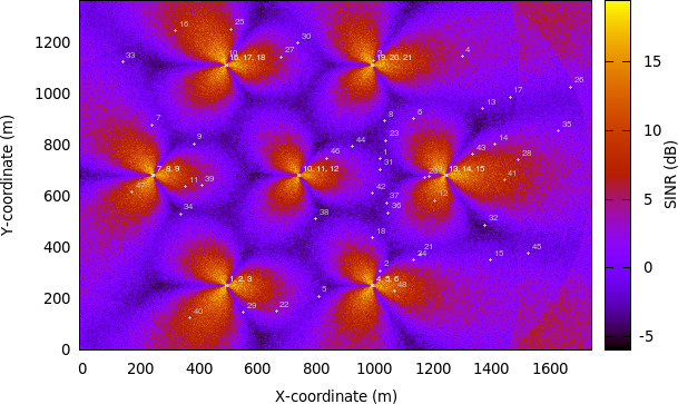
REM obtained from a simulation in handover campaign
After hours of running, the simulation campaign will eventually end. Next we will perform some post-processing on the produced simulation output to obtain meaningful information out of it.
In this example, we use GNU Octave to assist the processing of throughput and SINR data, as demonstrated in a sample GNU Octave script below:
% RxBytes is the 10th column
DlRxBytes = load ("no-op-DlRlcStats.txt") (:,10);
DlAverageThroughputKbps = sum (DlRxBytes) * 8 / 1000 / 50

% RxBytes is the 10th column
UlRxBytes = load ("no-op-UlRlcStats.txt") (:,10);
UlAverageThroughputKbps = sum (UlRxBytes) * 8 / 1000 / 50

% Sinr is the 6th column
DlSinr = load ("no-op-DlRsrpSinrStats.txt") (:,6);
% eliminate NaN values
idx = isnan (DlSinr);
DlSinr (idx) = 0;
DlAverageSinrDb = 10 * log10 (mean (DlSinr)) % convert to dB

% Sinr is the 5th column
UlSinr = load ("no-op-UlSinrStats.txt") (:,5);
% eliminate NaN values
idx = isnan (UlSinr);
UlSinr (idx) = 0;
UlAverageSinrDb = 10 * log10 (mean (UlSinr)) % convert to dB
As for the number of handovers, we can use simple shell scripting to count the number of occurrences of string “Handover” in the log file:
$ grep "Handover" no-op.txt | wc -l
Table Results of handover campaign below shows the complete statistics
after we are done with post-processing on every individual simulation run. The
values shown are the average of the results obtained from RngRun of 1, 2, 3,
and 4.
Statistics |
No-op |
A2-A4-RSRQ |
Strongest cell |
|---|---|---|---|
Average DL system throughput |
6 615 kbps |
20 509 kbps |
19 709 kbps |
Average UL system throughput |
4 095 kbps |
5 705 kbps |
6 627 kbps |
Average DL SINR |
-0.10 dB |
5.19 dB |
5.24 dB |
Average UL SINR |
9.54 dB |
81.57 dB |
79.65 dB |
Number of handovers per UE per second |
0 |
0.05694 |
0.04771 |
The results show that having a handover algorithm in a mobility simulation improves both user throughput and SINR significantly. There is little difference between the two handover algorithms in this campaign scenario. It would be interesting to see their performance in different scenarios, such as scenarios with home eNodeBs deployment.
19.2.23.2. Frequency Reuse examples
There are two examples showing Frequency Reuse Algorithms functionality.
lena-frequency-reuse is simple example with 3 eNBs in triangle layout.
There are 3 cell edge UEs, which are located in the center of this triangle and
3 cell center UEs (one near each eNB). User can also specify the number of randomly
located UEs. FR algorithm is installed in eNBs and each eNB has different FrCellTypeId,
what means each eNB uses different FR configuration. User can run lena-frequency-reuse
with 6 different FR algorithms: NoOp, Hard FR, Strict FR, Soft FR, Soft FFR and Enhanced FFR.
To run scenario with Distributed FFR algorithm, user should use lena-distributed-ffr.
These two examples are very similar, but they were split because Distributed FFR requires
EPC to be used, and other algorithms do not.
To run lena-frequency-reuse with different Frequency Reuse algorithms, user needs to specify
FR algorithm by overriding the default attribute ns3::LteHelper::FfrAlgorithm.
Example command to run lena-frequency-reuse with Soft FR algorithm is presented below:
$ ./ns3 run "lena-frequency-reuse --ns3::LteHelper::FfrAlgorithm=ns3::LteFrSoftAlgorithm"
In these examples functionality to generate REM and spectrum analyzer trace was added.
User can enable generation of it by setting generateRem and generateSpectrumTrace
attributes.
Command to generate REM for RB 1 in data channel from lena-frequency-reuse scenario
with Soft FR algorithm is presented below:
$ ./ns3 run "lena-frequency-reuse --ns3::LteHelper::FfrAlgorithm=ns3::LteFrSoftAlgorithm
  --generateRem=true --remRbId=1"
Radio Environment Map for Soft FR is presented in Figure REM for RB 1 obtained from lena-frequency-reuse example with Soft FR algorithm enabled.
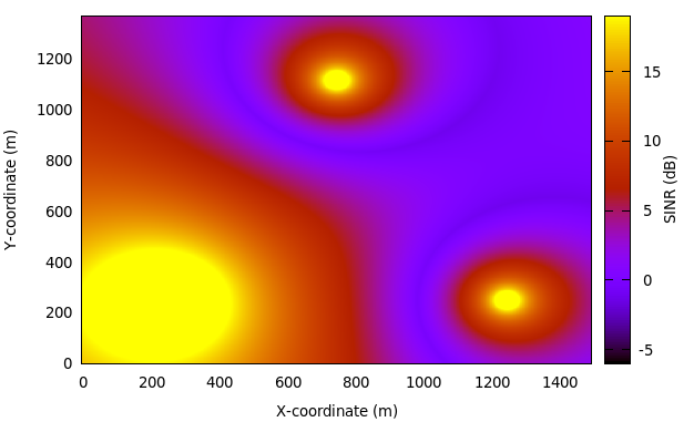
REM for RB 1 obtained from lena-frequency-reuse example with Soft FR
algorithm enabled
Command to generate spectrum trace from lena-frequency-reuse scenario
with Soft FFR algorithm is presented below (Spectrum Analyzer position needs to be configured
inside script):
$ ./ns3 run "lena-frequency-reuse --ns3::LteHelper::FfrAlgorithm=ns3::LteFfrSoftAlgorithm
  --generateSpectrumTrace=true"
Example spectrum analyzer trace is presented in figure Spectrum Analyzer trace obtained from lena-frequency-reuse example with Soft FFR algorithm enabled. Spectrum Analyzer was located need eNB with FrCellTypeId 2.. As can be seen, different data channel subbands are sent with different power level (according to configuration), while control channel is transmitted with uniform power along entire system bandwidth.
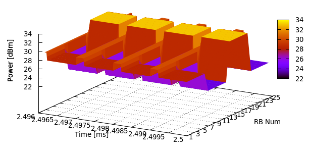
Spectrum Analyzer trace obtained from lena-frequency-reuse example
with Soft FFR algorithm enabled. Spectrum Analyzer was located need eNB
with FrCellTypeId 2.
lena-dual-stripe can be also run with Frequency Reuse algorithms installed in all macro eNB.
User needs to specify FR algorithm by overriding the default attribute ns3::LteHelper::FfrAlgorithm.
Example command to run lena-dual-stripe with Hard FR algorithm is presented below:
$ ./ns3 run "lena-dual-stripe
  --simTime=50 --nBlocks=0 --nMacroEnbSites=7 --nMacroEnbSitesX=2
  --epc=1 --useUdp=0 --outdoorUeMinSpeed=16.6667 --outdoorUeMaxSpeed=16.6667
  --ns3::LteHelper::HandoverAlgorithm=ns3::NoOpHandoverAlgorithm
  --ns3::LteHelper::FfrAlgorithm=ns3::LteFrHardAlgorithm
  --ns3::RadioBearerStatsCalculator::DlRlcOutputFilename=no-op-DlRlcStats.txt
  --ns3::RadioBearerStatsCalculator::UlRlcOutputFilename=no-op-UlRlcStats.txt
  --ns3::PhyStatsCalculator::DlRsrpSinrFilename=no-op-DlRsrpSinrStats.txt
  --ns3::PhyStatsCalculator::UlSinrFilename=no-op-UlSinrStats.txt
  --RngRun=1" > no-op.txt
Example command to generate REM for RB 1 in data channel from lena-dual-stripe scenario
with Hard FR algorithm is presented below:
$ ./ns3 run "lena-dual-stripe
  --simTime=50 --nBlocks=0 --nMacroEnbSites=7 --nMacroEnbSitesX=2
  --epc=0 --useUdp=0 --outdoorUeMinSpeed=16.6667 --outdoorUeMaxSpeed=16.6667
  --ns3::LteHelper::HandoverAlgorithm=ns3::NoOpHandoverAlgorithm
  --ns3::LteHelper::FfrAlgorithm=ns3::LteFrHardAlgorithm
  --ns3::RadioBearerStatsCalculator::DlRlcOutputFilename=no-op-DlRlcStats.txt
  --ns3::RadioBearerStatsCalculator::UlRlcOutputFilename=no-op-UlRlcStats.txt
  --ns3::PhyStatsCalculator::DlRsrpSinrFilename=no-op-DlRsrpSinrStats.txt
  --ns3::PhyStatsCalculator::UlSinrFilename=no-op-UlSinrStats.txt
  --RngRun=1 --generateRem=true --remRbId=1" > no-op.txt
Radio Environment Maps for RB 1, 10 and 20 generated from lena-dual-stripe
scenario with Hard Frequency Reuse algorithm are presented in the figures
below. These RB were selected because each one is used by different FR cell type.
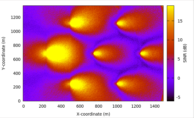
REM for RB 1 obtained from lena-dual-stripe simulation with Hard FR algorithm enabled
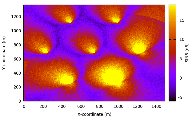
REM for RB 10 obtained from lena-dual-stripe simulation with Hard FR algorithm enabled
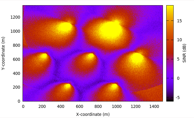
REM for RB 20 obtained from lena-dual-stripe simulation with Hard FR algorithm enabled
19.2.24. Carrier aggregation examples
The carrier aggregation feature is not enabled by default. The user can enable it by setting the boolean attribute
ns3::LteHelper::UseCa to true. The number of component carriers to be used in carrier aggregation can
be configured by setting the attribute ns3::LteHelper::NumberOfComponentCarriers. Currently the
maximum number is 5. Additionally, the component carrier manager needs to be configured. By default
the NoOpComponentCarrierManager is selected, which means that only the primary carrier is enabled. The Component
carrier manager (CCM) implementation that uses all the available carriers is RrComponentCarrierManager.
The CCM can be configured by using the attribute LteHelper::EnbComponentCarrierManager.
An example configuration is presented below:
Config::SetDefault("ns3::LteHelper::UseCa", BooleanValue(useCa));
Config::SetDefault("ns3::LteHelper::NumberOfComponentCarriers", UintegerValue(2));
Config::SetDefault("ns3::LteHelper::EnbComponentCarrierManager", StringValue("ns3::RrComponentCarrierManager"));
As an example, the user can take a look and run the lena-simple and lena-simple-epc programs and enable LTE traces
to check the performance. A new column is added to PHY and MAC traces to indicate the component carrier.
The test suite lte-carrier-aggregation is also a test program that can be used as an example as it can be run in a mode to write results
to output files by setting the s_writeResults boolean static variable to true. The test can be run by using a test-runner:
./ns3 run ‘test-runner –suite=lte-carrier-aggregation’
To plot the test results, a file has to be created in the root folder of the ns-3 repository, and added to it with the following content :
set terminal png set xlabel “Number of users” set ylabel “Throughput per UE [Mbps]” set key top right
downlink_results=”carrier_aggregation_results_dl.txt” uplink_results=”carrier_aggregation_results_ul.txt”
set output “ca-test-example-dl.png” set title “Downlink performance”
- plot downlink_results using 1:($2==1 ? $3/10000001/0) w lp t ‘NO SDL’,
downlink_results using 1:($2==2 ? $3/1000000 : 1/0) w lp t ‘RR SDL 1’, downlink_results using 1:($2==3 ? $3/1000000 : 1/0) w lp t ‘RR SDL 2’
set output “ca-test-example-ul.png” set title “Uplink performance”
- plot uplink_results using 1:($2==1 ? $3/10000001/0) w lp t ‘NO SDL’,
uplink_results using 1:($2==2 ? $3/1000000 : 1/0) w lp t ‘RR SDL 1’, uplink_results using 1:($2==3 ? $3/1000000 : 1/0) w lp t ‘RR SDL 2’
gnuplot can be run by providing the file name, so that in the ns-3 root directory
figures are generated. An example to run this test suite is shown in figures:
fig-ca-test-example-ul and fig-ca-test-example-dl.
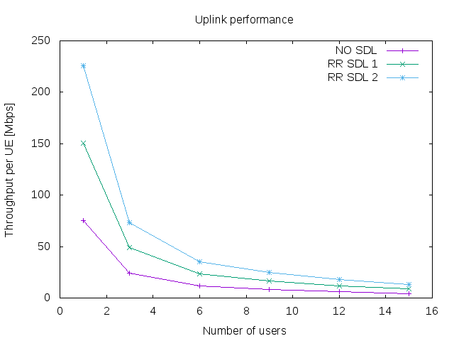
Example of CA test performance in the uplink
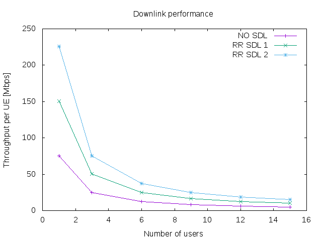
Example of CA test performance in the downlink
19.2.25. Radio link failure example
The example lena-radio-link-failure.cc is an example to simulate the RLF functionality. In particular, it simulates only one moving UE using Ideal or Real RRC protocol with EPC performing downlink and uplink communication in two scenarios shown in Scenario A: Radio link failure example with one eNB and Scenario B: Radio link failure example with two eNBs
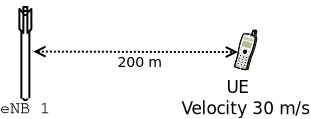
Scenario A: Radio link failure example with one eNB
We note that, the RLF detection is enabled by default, which can be disabled by
configuring the LteUePhy::EnableRlfDetection to false, e.g.,:
Config::SetDefault("ns3::LteUePhy::EnableRlfDetection", BooleanValue(false));
In this example, to study the impact of a RLF on the user’s quality of experience, we compute an instantaneous (i.e., every 200 ms) DL throughput of the UE, and writes it into a file for plotting purposes. For example, to simulate the “Scenario A” with Ideal and Real RRC protocol a user can use the following commands:
Ideal RRC:
./ns3 run "lena-radio-link-failure
--numberOfEnbs=1 --useIdealRrc=1
--interSiteDistance=1200 --n310=1 --n311=1
--t310=1 --enableCtrlErrorModel=1
--enableDataErrorModel=1 --simTime=25"

Real RRC:
./ns3 run "lena-radio-link-failure
--numberOfEnbs=1 --useIdealRrc=0
--interSiteDistance=1200 --n310=1 --n311=1
--t310=1 --enableCtrlErrorModel=1
--enableDataErrorModel=1 --simTime=25"
After running the above two commands, we can use a simple gnuplot script to plot the throughput as shown in the Figure Downlink instantaneous throughput of UE in scenario A , e.g.,
set terminal png
set output  "lena-radio-link-failure-one-enb-thrput.png"
set multiplot
set xlabel "Time [s]"
set ylabel "Instantaneous throughput UE [Mbps]"
set grid
set title "LTE RLF example 1 eNB DL instantaneous throughput"
plot "rlf_dl_thrput_1_eNB_ideal_rrc" using ($1):($2) with linespoints
title 'Ideal RRC' linestyle 1 lw 2 lc rgb 'blue', "rlf_dl_thrput_1_eNB_real_rrc"
using ($1):($2) with linespoints title 'Real RRC' linestyle 2 lw 2 lc rgb 'red'

unset multiplot
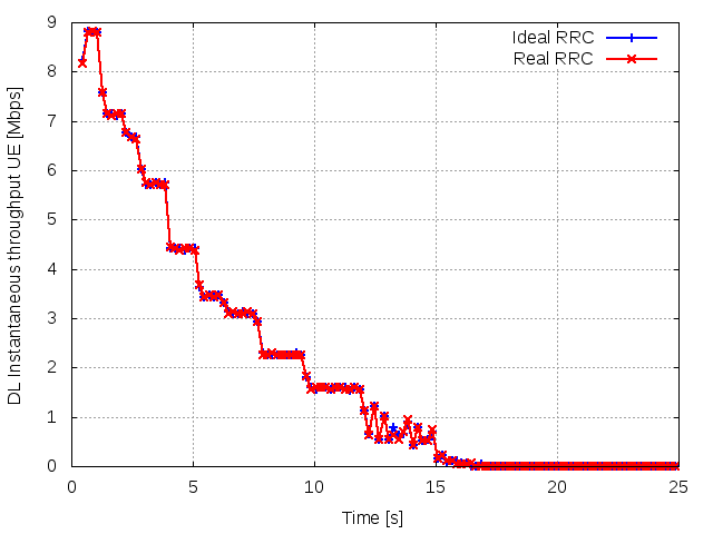
Downlink instantaneous throughput of UE in scenario A
In the simulator, a UE can synchronize (i.e., start reading system information) with an eNB at a low RSRP level, which defaults to -140 dBm (see QRxLevMin attribute of eNB RRC). It enables the UE to start the random access procedure with the eNB. In this scenario, when using the Ideal RRC the UE after the RLF will connect and disconnect from the eNB several times. This is because in the Ideal RRC mode, once the UE is able to receive Random Access Response (RAR) from the eNB, it can complete the RRC connection establishment procedure (RRC connection establishment) without any errors, since all the RRC messages are exchanged ideally between the eNB and the UE. However, soon after the connection establishment, it ends up in RLF due to the poor channel quality. On the other hand, with the Real RRC the UE after the RLF will not be able to complete the RRC connection establishment procedure due to the loss of RRC messages. Thus, it will not be able to establish the connection with the eNB. Therefore, in both the cases the UE throughput drops to zero as shown in the Figure Downlink instantaneous throughput of UE in scenario A. It is also worthwhile to mention that towards the end of the simulation (using Ideal or Real RRC) there are occasions where RAR timer at the UE MAC would timeout due to the increased distance between the eNB and the UE, which causes errors while decoding this message at the UE (Note: the downlink control error model is enabled by default).
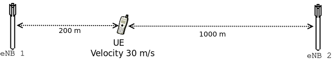
Scenario B: Radio link failure example with two eNBs
Similarly, to simulate the “Scenario B” with Ideal and Real RRC protocol following commands can be used:
Ideal RRC:
./ns3 run "lena-radio-link-failure
--numberOfEnbs=2 --useIdealRrc=1
--interSiteDistance=1200 --n310=1 --n311=1
--t310=1 --enableCtrlErrorModel=1
--enableDataErrorModel=1 --simTime=25"

Real RRC:
./ns3 run "lena-radio-link-failure
--numberOfEnbs=2 --useIdealRrc=0
--interSiteDistance=1200 --n310=1 --n311=1
--t310=1 --enableCtrlErrorModel=1
--enableDataErrorModel=1 --simTime=25"
Figure Downlink instantaneous throughput of UE in scenario B, shows the throughput in “Scenario B”. We note that in this scenario the handover algorithm is not used. As expected, with Ideal RRC protocol the UE after the RLF can complete the random access procedure with the second eNB. Interestingly, the DL SINR after the connection establishment is not low enough to trigger the RLF, but it is low enough to impact the DL control reception for some TBs, which in turn causes loss of data. It can be observed from the slightly unstable throughput of the UE after connecting to the second eNB. On the other hand, with Real RRC the UE faces problems in connection establishment phase due to the loss of RRC messages, in particular, the RRC connection request from the UE. This is the reason why the UE throughput after the RLF remains zero for a more extended period as compared to the ideal RRC protocol.
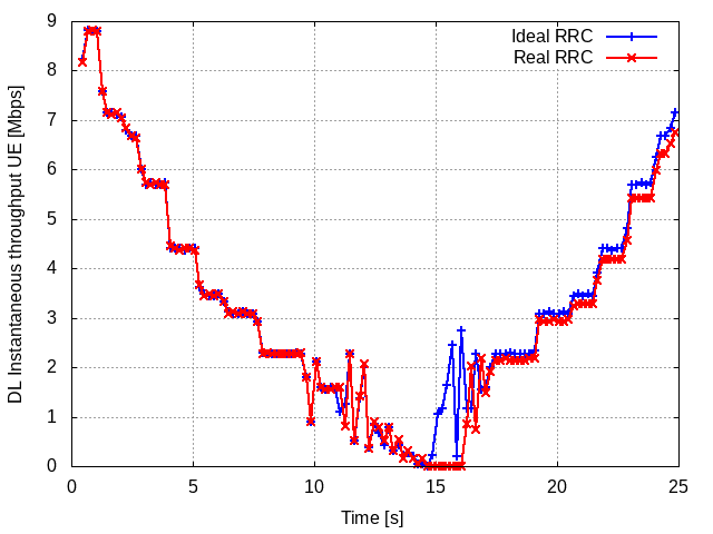
Downlink instantaneous throughput of UE in scenario B
19.2.26. Troubleshooting and debugging tips
Many users post on the ns-3-users mailing list asking, for example, why they do not get any traffic in their simulation, or maybe only uplink but no downlink traffic is generated, etc. In most of the cases, this is a bug in the user simulation program. Here the reader can find some tips to debug the program and find out the cause of the problem.
The general approach is to selectively and incrementally enable the logging of relevant LTE module components, verifying upon each activation that the output is as expected. In detail:
first check the control plane, in particular the RRC connection establishment procedure, by enabling the log components LteUeRrc and LteEnbRrc
then check packet transmissions on the data plane, starting by enabling the log components LteUeNetDevice and the EpcSgwApplication, EpcPgwApplication and EpcEnbApplication, then moving down the LTE radio stack (PDCP, RLC, MAC, and finally PHY). All this until you find where packets stop being processed / forwarded.