
|
A Discrete-Event Network Simulator
|
Models |
|
|
A Discrete-Event Network Simulator
|
Models |
We assume the reader is already familiar with how to use the ns-3 simulator to run generic simulation programs. If this is not the case, we strongly recommend the reader to consult [ns3tutorial].
The ns-3 LTE model is a software library that allows the simulation of LTE networks, optionally including the Evolved Packet Core (EPC). The process of performing such simulations typically involves the following steps:
- Define the scenario to be simulated
- Write a simulation program that recreates the desired scenario topology/architecture. This is done accessing the ns-3 LTE model library using the ns3::LteHelper API defined in src/lte/helper/lte-helper.h.
- Specify configuration parameters of the objects that are being used for the simulation. This can be done using input files (via the ns3::ConfigStore) or directly within the simulation program.
- Configure the desired output to be produced by the simulator
- Run the simulation.
All these aspects will be explained in the following sections by means of practical examples.
Here is the minimal simulation program that is needed to do an LTE-only simulation (without EPC).
Initial boilerplate:
#include "ns3/core-module.h"
#include "ns3/network-module.h"
#include "ns3/mobility-module.h"
#include "ns3/lte-module.h"

using namespace ns3;

int main (int argc, char *argv[])
{
  // the rest of the simulation program follows
Create a LteHelper object:
Ptr<LteHelper> lteHelper = CreateObject<LteHelper> ();
This will instantiate some common objects (e.g., the Channel object) and provide the methods to add eNBs and UEs and configure them.
Create Node objects for the eNB(s) and the UEs:
NodeContainer enbNodes;
enbNodes.Create (1);
NodeContainer ueNodes;
ueNodes.Create (2);
Note that the above Node instances at this point still don’t have an LTE protocol stack installed; they’re just empty nodes.
Configure the Mobility model for all the nodes:
MobilityHelper mobility;
mobility.SetMobilityModel ("ns3::ConstantPositionMobilityModel");
mobility.Install (enbNodes);
mobility.SetMobilityModel ("ns3::ConstantPositionMobilityModel");
mobility.Install (ueNodes);
The above will place all nodes at the coordinates (0,0,0). Please refer to the documentation of the ns-3 mobility model for how to set your own position or configure node movement.
Install an LTE protocol stack on the eNB(s):
NetDeviceContainer enbDevs;
enbDevs = lteHelper->InstallEnbDevice (enbNodes);
Install an LTE protocol stack on the UEs:
NetDeviceContainer ueDevs;
ueDevs = lteHelper->InstallUeDevice (ueNodes);
Attach the UEs to an eNB. This will configure each UE according to the eNB configuration, and create an RRC connection between them:
lteHelper->Attach (ueDevs, enbDevs.Get (0));
Activate an EPS Bearer including the setup of the Radio Bearer between an eNB and its attached UE:
enum EpsBearer::Qci q = EpsBearer::GBR_CONV_VOICE;
EpsBearer bearer (q);
lteHelper->ActivateEpsBearer (ueDevs, bearer);
In the current version of the ns-3 LTE model, the activation of an EPS Bearer will also activate two saturation traffic generators for that bearer, one in uplink and one in downlink.
Set the stop time:
Simulator::Stop (Seconds (0.005));
This is needed otherwise the simulation will last forever, because (among others) the start-of-subframe event is scheduled repeatedly, and the ns-3 simulator scheduler will hence never run out of events.
Run the simulation:
Simulator::Run ();
Cleanup and exit:
Simulator::Destroy ();
return 0;
}
For how to compile and run simulation programs, please refer to [ns3tutorial].
All the relevant LTE model parameters are managed through the ns-3 attribute system. Please refer to the [ns3tutorial] and [ns3manual] for detailed information on all the possible methods to do it (environmental variables, C++ API, GtkConfigStore...).
In the following, we just briefly summarize how to do it using input files together with the ns-3 ConfigStore. First of all, you need to put the following in your simulation program, right after main () starts:
CommandLine cmd;
cmd.Parse (argc, argv);
ConfigStore inputConfig;
inputConfig.ConfigureDefaults ();
// parse again so you can override default values from the command line
cmd.Parse (argc, argv);
for the above to work, make sure you also #include "ns3/config-store.h". Now create a text file named (for example) input-defaults.txt specifying the new default values that you want to use for some attributes:
default ns3::LteHelper::Scheduler "ns3::PfFfMacScheduler"
default ns3::LteHelper::PathlossModel "ns3::FriisSpectrumPropagationLossModel"
default ns3::LteEnbNetDevice::UlBandwidth "25"
default ns3::LteEnbNetDevice::DlBandwidth "25"
default ns3::LteEnbNetDevice::DlEarfcn "100"
default ns3::LteEnbNetDevice::UlEarfcn "18100"
default ns3::LteUePhy::TxPower "10"
default ns3::LteUePhy::NoiseFigure "9"
default ns3::LteEnbPhy::TxPower "30"
default ns3::LteEnbPhy::NoiseFigure "5"
Supposing your simulation program is called src/lte/examples/lte-sim-with-input, you can now pass these settings to the simulation program in the following way:
./waf --command-template="%s --ns3::ConfigStore::Filename=input-defaults.txt --ns3::ConfigStore::Mode=Load --ns3::ConfigStore::FileFormat=RawText" --run src/lte/examples/lte-sim-with-input
Furthermore, you can generate a template input file with the following command:
./waf --command-template="%s --ns3::ConfigStore::Filename=input-defaults.txt --ns3::ConfigStore::Mode=Save --ns3::ConfigStore::FileFormat=RawText" --run src/lte/examples/lte-sim-with-input
note that the above will put in the file input-defaults.txt all the default values that are registered in your particular build of the simulator, including lots of non-LTE attributes.
The ns-3 LTE model currently supports the output to file of MAC, RLC and PDCP level Key Performance Indicators (KPIs). You can enable it in the following way:
Ptr<LteHelper> lteHelper = CreateObject<LteHelper> ();

// configure all the simulation scenario here...

lteHelper->EnableMacTraces ();
lteHelper->EnableRlcTraces ();
lteHelper->EnablePdcpTraces ();

Simulator::Run ();
RLC and PDCP KPIs are calculated over a time interval and stored on ASCII files, two for RLC KPIs and two for PDCP KPIs, in each case one for uplink and one for downlink. The time interval duration can be controlled using the attribute ns3::RadioBearerStatsCalculator::EpochDuration.
The columns of the RLC KPI files is the following (the same for uplink and downlink):
- start time of measurement interval in seconds since the start of simulation
- end time of measurement interval in seconds since the start of simulation
- Cell ID
- unique UE ID (IMSI)
- cell-specific UE ID (RNTI)
- Logical Channel ID
- Number of transmitted RLC PDUs
- Total bytes transmitted.
- Number of received RLC PDUs
- Total bytes received
- Average RLC PDU delay in seconds
- Standard deviation of the RLC PDU delay
- Minimum value of the RLC PDU delay
- Maximum value of the RLC PDU delay
- Average RLC PDU size, in bytes
- Standard deviation of the RLC PDU size
- Minimum RLC PDU size
- Maximum RLC PDU size
Similarly, the columns of the PDCP KPI files is the following (again, the same for uplink and downlink):
- start time of measurement interval in seconds since the start of simulation
- end time of measurement interval in seconds since the start of simulation
- Cell ID
- unique UE ID (IMSI)
- cell-specific UE ID (RNTI)
- Logical Channel ID
- Number of transmitted PDCP PDUs
- Total bytes transmitted.
- Number of received PDCP PDUs
- Total bytes received
- Average PDCP PDU delay in seconds
- Standard deviation of the PDCP PDU delay
- Minimum value of the PDCP PDU delay
- Maximum value of the PDCP PDU delay
- Average PDCP PDU size, in bytes
- Standard deviation of the PDCP PDU size
- Minimum PDCP PDU size
- Maximum PDCP PDU size
MAC KPIs are basically a trace of the resource allocation reported by the scheduler upon the start of every subframe. They are stored in ASCII files. For downlink MAC KPIs the format is the following:
- Simulation time in seconds at which the allocation is indicated by the scheduler
- Cell ID
- unique UE ID (IMSI)
- Frame number
- Subframe number
- cell-specific UE ID (RNTI)
- MCS of TB 1
- size of TB 1
- MCS of TB 2 (0 if not present)
- size of TB 2 (0 if not present)
while for uplink MAC KPIs the format is:
- Simulation time in seconds at which the allocation is indicated by the scheduler
- Cell ID
- unique UE ID (IMSI)
- Frame number
- Subframe number
- cell-specific UE ID (RNTI)
- MCS of TB
- size of TB
The names of the files used for MAC KPI output can be customized via the ns-3 attributes ns3::MacStatsCalculator::DlOutputFilename and ns3::MacStatsCalculator::UlOutputFilename.
In this section we will describe how to use fading traces within LTE simulations.
It is possible to generate fading traces by using a dedicated matlab script provided with the code (/lte/model/fading-traces/fading-trace-generator.m). This script already includes the typical taps configurations for three 3GPP scenarios (i.e., pedestrian, vehicular and urban as defined in Annex B.2 of [TS36104]); however users can also introduce their specific configurations. The list of the configurable parameters is provided in the following:
- fc : the frequency in use (it affects the computation of the doppler speed).
- v_km_h : the speed of the users
- traceDuration : the duration in seconds of the total length of the trace.
- numRBs : the number of the resource block to be evaluated.
- tag : the tag to be applied to the file generated.
The file generated contains ASCII-formatted real values organized in a matrix fashion: every row corresponds to a different RB, and every column correspond to a different temporal fading trace sample.
It has to be noted that the ns-3 LTE module is able to work with any fading trace file that complies with the above described ASCII format. Hence, other external tools can be used to generate custom fading traces, such as for example other simulators or experimental devices.
When using a fading trace, it is of paramount importance to specify correctly the trace parameters in the simulation, so that the fading model can load and use it correcly. The parameters to be configured are:
- TraceFilename : the name of the trace to be loaded (absolute path, or relative path w.r.t. the path from where the simulation program is executed);
- TraceLength : the trace duration in seconds;
- SamplesNum : the number of samples;
- WindowSize : the size of the fading sampling window in seconds;
It is important to highlight that the sampling interval of the fading trace has to be 1 ms or greater, and in the latter case it has to be an integer multiple of 1 ms in order to be correctly processed by the fading module.
The default configuration of the matlab script provides a trace 10 seconds long, made of 10,000 samples (i.e., 1 sample per TTI=1ms) and used with a windows size of 0.5 seconds amplitude. These are also the default values of the parameters above used in the simulator; therefore their settage can be avoided in case the fading trace respects them.
In order to activate the fading module (which is not active by default) the following code should be included in the simulation program:
Ptr<LteHelper> lteHelper = CreateObject<LteHelper> ();
lteHelper->SetFadingModel("ns3::TraceFadingLossModel");
And for setting the parameters:
lteHelper->SetFadingModelAttribute ("TraceFilename", StringValue ("src/lte/model/fading-traces/fading_trace_EPA_3kmph.fad"));
lteHelper->SetFadingModelAttribute ("TraceLength", TimeValue (Seconds (10.0)));
lteHelper->SetFadingModelAttribute ("SamplesNum", UintegerValue (10000));
lteHelper->SetFadingModelAttribute ("WindowSize", TimeValue (Seconds (0.5)));
lteHelper->SetFadingModelAttribute ("RbNum", UintegerValue (100));
It has to be noted that, TraceFilename does not have a default value, therefore is has to be always set explicitly.
The simulator provide natively three fading traces generated according to the configurations defined in in Annex B.2 of [TS36104]. These traces are available in the folder src/lte/model/fading-traces/). An excerpt from these traces is represented in the following figures.
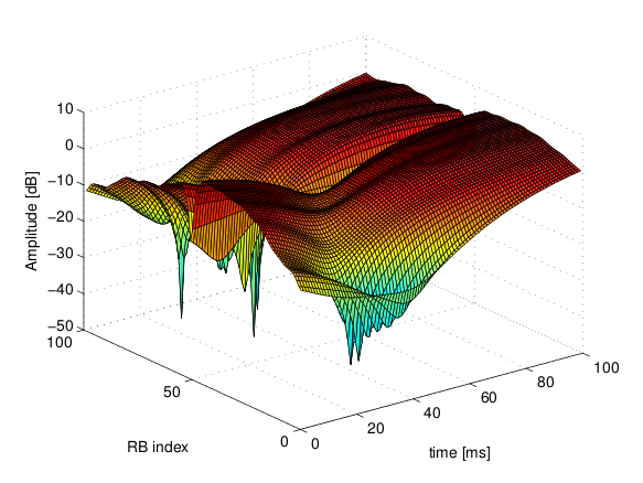
Excerpt of the fading trace included in the simulator for a pedestrian scenario (speed of 3 kmph).
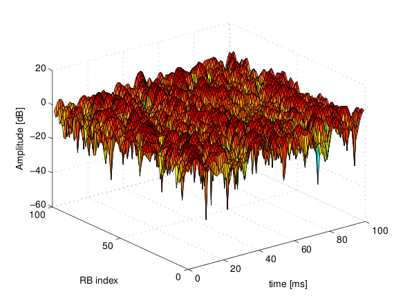
Excerpt of the fading trace included in the simulator for a vehicular scenario (speed of 60 kmph).
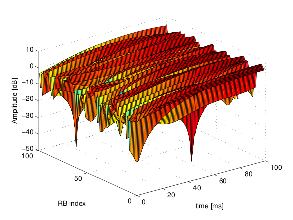
Excerpt of the fading trace included in the simulator for an urban scenario (speed of 3 kmph).
We now explain by examples how to use the buildings model (in particular, the BuildingMobilityModel and the BuildingPropagationModel classes) in an ns-3 simulation program to setup an LTE simulation scenario that includes buildings and indoor nodes.
Header files to be included:
#include <ns3/buildings-mobility-model.h>
#include <ns3/buildings-propagation-loss-model.h>
#include <ns3/building.h>
Pathloss model selection:
Ptr<LteHelper> lteHelper = CreateObject<LteHelper> ();

lteHelper->SetAttribute ("PathlossModel", StringValue ("ns3::BuildingsPropagationLossModel"));
EUTRA Band Selection
The selection of the working frequency of the propagation model has to be done with the standard ns-3 attribute system as described in the correspond section (“Configuration of LTE model parameters”) by means of the DlEarfcn and UlEarfcn parameters, for instance:
lteHelper->SetEnbDeviceAttribute ("DlEarfcn", UintegerValue (100));
lteHelper->SetEnbDeviceAttribute ("UlEarfcn", UintegerValue (18100));
It is to be noted that using other means to configure the frequency used by the propagation model (i.e., configuring the corresponding BuildingsPropagationLossModel attributes directly) might generates conflicts in the frequencies definition in the modules during the simulation, and is therefore not advised.
Mobility model selection:
MobilityHelper mobility;
mobility.SetMobilityModel ("ns3::BuildingsMobilityModel");
Building creation:
double x_min = 0.0;
double x_max = 10.0;
double y_min = 0.0;
double y_max = 20.0;
double z_min = 0.0;
double z_max = 10.0;
Ptr<Building> b = CreateObject <Building> ();
b->SetBoundaries (Box (x_min, x_max, y_min, y_max, z_min, z_max));
b->SetBuildingType (Building::Residential);
b->SetExtWallsType (Building::ConcreteWithWindows);
b->SetNFloors (3);
b->SetNRoomsX (3);
b->SetNRoomsY (2);
This will instantiate a residential building with base of 10 x 20 meters and height of 10 meters whose external walls are of concrete with windows; the building has three floors and has an internal 3 x 2 grid of rooms of equal size.
Node creation and positioning:
ueNodes.Create (2);
mobility.Install (ueNodes);
NetDeviceContainer ueDevs;
ueDevs = lteHelper->InstallUeDevice (ueNodes);
Ptr<BuildingsMobilityModel> mm0 = enbNodes.Get (0)->GetObject<BuildingsMobilityModel> ();
Ptr<BuildingsMobilityModel> mm1 = enbNodes.Get (1)->GetObject<BuildingsMobilityModel> ();
mm0->SetPosition (Vector (5.0, 5.0, 1.5));
mm1->SetPosition (Vector (30.0, 40.0, 1.5));
This positions the node on the scenario. Note that, in this example, node 0 will be in the building, and node 1 will be out of the building. Note that this alone is not sufficient to setup the topology correctly. What is left to be done is to issue the following command after we have placed all nodes in the simulation:
BuildingsHelper::MakeMobilityModelConsistent ();
This command will go through the lists of all nodes and of all buildings, determine for each user if it is indoor or outdoor, and if indoor it will also determine the building in which the user is located and the corresponding floor and number inside the building.
Is this subsection we illustrate how to configure the MIMO parameters. LTE defines 7 types of transmission modes:
- Transmission Mode 1: SISO.
- Transmission Mode 2: MIMO Tx Diversity.
- Transmission Mode 3: MIMO Spatial Multiplexity Open Loop.
- Transmission Mode 4: MIMO Spatial Multiplexity Closed Loop.
- Transmission Mode 5: MIMO Multi-User.
- Transmission Mode 6: Closer loop single layer precoding.
- Transmission Mode 7: Single antenna port 5.
According to model implemented, the simulator includes the first three transmission modes types. The default one is the Transmission Mode 1 (SISO). In order to change the default Transmission Mode to be used, the attribute DefaultTransmissionMode of the LteEnbRrc can be used, as shown in the following:
Config::SetDefault ("ns3::LteEnbRrc::DefaultTransmissionMode", UintegerValue (0)); // SISO
Config::SetDefault ("ns3::LteEnbRrc::DefaultTransmissionMode", UintegerValue (1)); // MIMO Tx diversity (1 layer)
Config::SetDefault ("ns3::LteEnbRrc::DefaultTransmissionMode", UintegerValue (2)); // MIMO Spatial Multiplexity (2 layers)
For changing the transmission mode of a certain user during the simulation a specific interface has been implemented in both standard schedulers:
void TransmissionModeConfigurationUpdate (uint16_t rnti, uint8_t txMode);
This method can be used both for developing transmission mode decision engine (i.e., for optimizing the transmission mode according to channel condition and/or user’s requirements) and for manual switching from simulation script. In the latter case, the switching can be done as shown in the following:
Ptr<LteEnbNetDevice> lteEnbDev = enbDevs.Get (0)->GetObject<LteEnbNetDevice> ();
PointerValue ptrval;
enbNetDev->GetAttribute ("FfMacScheduler", ptrval);
Ptr<RrFfMacScheduler> rrsched = ptrval.Get<RrFfMacScheduler> ();
Simulator::Schedule (Seconds (0.2), &RrFfMacScheduler::TransmissionModeConfigurationUpdate, rrsched, rnti, 1);
Finally, the model implemented can be reconfigured according to different MIMO models by updating the gain values (the only constraints is that the gain has to be constant during simulation run-time and common for the layers). The gain of each Transmission Mode can be changed according to the standard ns3 attribute system, where the attributes are: TxMode1Gain, TxMode2Gain, TxMode3Gain, TxMode4Gain, TxMode5Gain, TxMode6Gain and TxMode7Gain. By default only TxMode1Gain, TxMode2Gain and TxMode3Gain have a meaningful value, that are the ones derived by _[CatreuxMIMO] (i.e., respectively 0.0, 4.2 and -2.8 dB).
We now show how associate a particular AntennaModel with an eNB device in order to model a sector of a macro eNB. For this purpose, it is convenient to use the CosineAntennaModel provided by the ns-3 antenna module. The configuration of the eNB is to be done via the LteHelper instance right before the creation of the EnbNetDevice, as shown in the following:
lteHelper->SetEnbAntennaModelType ("ns3::CosineAntennaModel");
lteHelper->SetEnbAntennaModelAttribute ("Orientation", DoubleValue (0));
lteHelper->SetEnbAntennaModelAttribute ("Beamwidth",   DoubleValue (60);
lteHelper->SetEnbAntennaModelAttribute ("MaxGain",     DoubleValue (0.0));
the above code will generate an antenna model with a 60 degrees
beamwidth pointing along the X axis. The orientation is measured
in degrees from the X axis, e.g., an orientation of 90 would point
along the Y axis, and an orientation of -90 would point in the
negative direction along the Y axis. The beamwidth is the -3 dB
beamwidth, e.g, for a 60 degree beamwidth the antenna gain at an angle
of  degrees from the direction of orientation is -3 dB.
To create a multi-sector site, you need to create different ns-3 nodes placed at the same position, and to configure separate EnbNetDevice with different antenna orientations to be installed on each node.
By using the class RadioEnvironmentMapHelper it is possible to output to a file a Radio Environment Map (REM), i.e., a uniform 2D grid of values that represent the Signal-to-noise ratio in the downlink with respect to the eNB that has the strongest signal at each point.
To do this, you just need to add the following code to your simulation program towards the end, right before the call to Simulator::Run ():
Ptr<RadioEnvironmentMapHelper> remHelper = CreateObject<RadioEnvironmentMapHelper> ();
remHelper->SetAttribute ("ChannelPath", StringValue ("/ChannelList/0"));
remHelper->SetAttribute ("OutputFile", StringValue ("rem.out"));
remHelper->SetAttribute ("XMin", DoubleValue (-400.0));
remHelper->SetAttribute ("XMax", DoubleValue (400.0));
remHelper->SetAttribute ("XRes", UintegerValue (100));
remHelper->SetAttribute ("YMin", DoubleValue (-300.0));
remHelper->SetAttribute ("YMax", DoubleValue (300.0));
remHelper->SetAttribute ("YRes", UintegerValue (75));
remHelper->SetAttribute ("Z", DoubleValue (0.0));
remHelper->Install ();
By configuring the attributes of the RadioEnvironmentMapHelper object as shown above, you can tune the parameters of the REM to be generated. Note that each RadioEnvironmentMapHelper instance can generate only one REM; if you want to generate more REMs, you need to create one separate instance for each REM.
Note that the REM generation is very demanding, in particular:
- the run-time memory consumption is approximately 5KB per pixel. For example, a REM with a resolution of 500x500 needs about 1.25 GB of memory, and a resolution of 1000x1000 needs about 5 GB (too much for a regular PC at the time of this writing).
- if you generate a REM at the beginning of a simulation, it will slow down the execution of the rest of the simulation. If you want to generate a REM for a program and also use the same program to get simulation result, it is recommended to add a command-line switch that allows to either generate the REM or run the complete simulation. For this purpose, note that there is an attribute RadioEnvironmentMapHelper::StopWhenDone (default: true) that will force the simulation to stop right after the REM has been generated.
The REM is stored in an ASCII file in the following format:
- column 1 is the x coordinate
- column 2 is the y coordinate
- column 3 is the z coordinate
- column 4 is the SINR in linear units
A minimal gnuplot script that allows you to plot the REM is given below:
set view map;
set xlabel "X"
set ylabel "Y"
set cblabel "SINR (dB)"
unset key
plot "rem.out" using ($1):($2):(10*log10($4)) with image
As an example, here is the REM that can be obtained with the example program lena-dual-stripe, which shows a three-sector LTE macrocell in a co-channel deployment with some residential femtocells randomly deployed in two blocks of apartments.
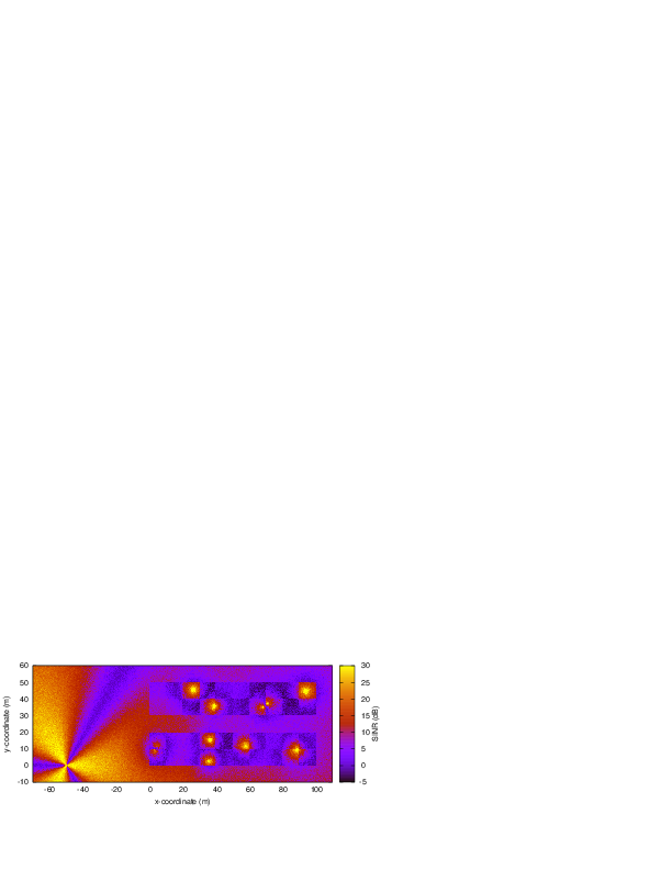
REM obtained from the lena-dual-stripe example
The simulator provides two possible schemes for what concerns the selection of the MCSs and correspondly the generation of the CQIs. The first one is based on the GSoC module [Piro2011] and works per RB basis. This model can be activated with the ns3 attribute system, as presented in the following:
Config::SetDefault ("ns3::LteAmc::AmcModel", EnumValue (LteAmc::PiroEW2010));
While, the solution based on the physical error model can be controlled with:
Config::SetDefault ("ns3::LteAmc::AmcModel", EnumValue (LteAmc::MiErrorModel));
Finally, the required efficiency of the PiroEW2010 AMC module can be tuned thanks to the Ber attribute (), for instance:
Config::SetDefault ("ns3::LteAmc::Ber", DoubleValue (0.00005));
We now explain how to write a simulation program that allows to simulate the EPC in addition to the LTE radio access network. The use of EPC allows to use IPv4 networking with LTE devices. In other words, you will be able to use the regular ns-3 applications and sockets over IPv4 over LTE, and also to connect an LTE network to any other IPv4 network you might have in your simulation.
First of all, in your simulation program you need to create two helpers:
Ptr<LteHelper> lteHelper = CreateObject<LteHelper> ();
Ptr<EpcHelper> epcHelper = CreateObject<EpcHelper> ();
Then, you need to tell the LTE helper that the EPC will be used:
lteHelper->SetEpcHelper (epcHelper);
the above step is necessary so that the LTE helper will trigger the appropriate EPC configuration in correspondance with some important configuration, such as when a new eNB or UE is added to the simulation, or an EPS bearer is created. The EPC helper will automatically take care of the necessary setup, such as S1 link creation and S1 bearer setup. All this will be done without the intervention of the user.
It is to be noted that, upon construction, the EpcHelper will also create and configure the PGW node. Its configuration in particular is very complex, and hence is done automatically by the Helper. Still, it is allowed to access the PGW node in order to connect it to other IPv4 network (e.g., the internet). Here is a very simple example about how to connect a single remote host to the PGW via a point-to-point link:
Ptr<Node> pgw = epcHelper->GetPgwNode ();

 // Create a single RemoteHost
NodeContainer remoteHostContainer;
remoteHostContainer.Create (1);
Ptr<Node> remoteHost = remoteHostContainer.Get (0);
InternetStackHelper internet;
internet.Install (remoteHostContainer);

// Create the internet
PointToPointHelper p2ph;
p2ph.SetDeviceAttribute ("DataRate", DataRateValue (DataRate ("100Gb/s")));
p2ph.SetDeviceAttribute ("Mtu", UintegerValue (1500));
p2ph.SetChannelAttribute ("Delay", TimeValue (Seconds (0.010)));
NetDeviceContainer internetDevices = p2ph.Install (pgw, remoteHost);
Ipv4AddressHelper ipv4h;
ipv4h.SetBase ("1.0.0.0", "255.0.0.0");
Ipv4InterfaceContainer internetIpIfaces = ipv4h.Assign (internetDevices);
// interface 0 is localhost, 1 is the p2p device
Ipv4Address remoteHostAddr = internetIpIfaces.GetAddress (1);
It’s important to specify routes so that the remote host can reach LTE UEs. One way of doing this is by exploiting the fact that the EpcHelper will by default assign to LTE UEs an IP address in the 7.0.0.0 network. With this in mind, it suffices to do:
Ipv4StaticRoutingHelper ipv4RoutingHelper;
Ptr<Ipv4StaticRouting> remoteHostStaticRouting = ipv4RoutingHelper.GetStaticRouting (remoteHost->GetObject<Ipv4> ());
remoteHostStaticRouting->AddNetworkRouteTo (Ipv4Address ("7.0.0.0"), Ipv4Mask ("255.0.0.0"), 1);
Now, you should go on and create LTE eNBs and UEs as explained in the previous sections. You can of course configure other LTE aspects such as pathloss and fading models. Right after you created the UEs, you should also configure them for IP networking. This is done as follows. We assume you have a container for UE and eNodeB nodes like this:
NodeContainer ueNodes;
NodeContainer enbNodes;
to configure an LTE-only simulation, you would then normally do something like this:
NetDeviceContainer ueLteDevs = lteHelper->InstallUeDevice (ueNodes);
lteHelper->Attach (ueLteDevs, enbLteDevs.Get (0));
in order to configure the UEs for IP networking, you just need to additionally do like this:
// we install the IP stack on the UEs
InternetStackHelper internet;
internet.Install (ueNodes);

// assign IP address to UEs
for (uint32_t u = 0; u < ueNodes.GetN (); ++u)
  {
    Ptr<Node> ue = ueNodes.Get (u);
    Ptr<NetDevice> ueLteDevice = ueLteDevs.Get (u);
    Ipv4InterfaceContainer ueIpIface = epcHelper->AssignUeIpv4Address (NetDeviceContainer (ueLteDevice));
    // set the default gateway for the UE
    Ptr<Ipv4StaticRouting> ueStaticRouting = ipv4RoutingHelper.GetStaticRouting (ue->GetObject<Ipv4> ());
    ueStaticRouting->SetDefaultRoute (epcHelper->GetUeDefaultGatewayAddress (), 1);
  }
The activation of bearers is done exactly in the same way as for an LTE-only simulation. Here is how to activate a default bearer:
lteHelper->ActivateEpsBearer (ueLteDevs, EpsBearer (EpsBearer::NGBR_VIDEO_TCP_DEFAULT), EpcTft::Default ());
you can of course use custom EpsBearer and EpcTft configurations, please refer to the doxygen documentation for how to do it.
Finally, you can install applications on the LTE UE nodes that communicate with remote applications over the internet. This is done following the usual ns-3 procedures. Following our simple example with a single remoteHost, here is how to setup downlink communication, with an UdpClient application on the remote host, and a PacketSink on the LTE UE (using the same variable names of the previous code snippets)
uint16_t dlPort = 1234;
PacketSinkHelper packetSinkHelper ("ns3::UdpSocketFactory", InetSocketAddress (Ipv4Address::GetAny (), dlPort));
ApplicationContainer serverApps = packetSinkHelper.Install (ue);
serverApps.Start (Seconds (0.01));
UdpClientHelper client (ueIpIface.GetAddress (0), dlPort);
ApplicationContainer clientApps = client.Install (remoteHost);
clientApps.Start (Seconds (0.01));
That’s all! You can now start your simulation as usual:
Simulator::Stop (Seconds (10.0));
Simulator::Run ();
The directory src/lte/examples/ contains some example simulation programs that show how to simulate different LTE scenarios.
There is a vast amount of reference LTE simulation scenarios which can be found in the literature. Here we list some of them:
- The dual stripe model [R4-092042], which is partially implemented in the example program src/lte/examples/lena-dual-stripe.cc
- The system simulation scenarios mentioned in section A.2 of [TR36814]