
|
A Discrete-Event Network Simulator
|
Models |
|
|
A Discrete-Event Network Simulator
|
Models |
To test and validate the ns-3 LTE module, several test suites are provided which are integrated with the ns-3 test framework. To run them, you need to have configured the build of the simulator in this way:
./waf configure --enable-tests --enable-modules=lte --enable-examples
./test.py
The above will run not only the test suites belonging to the LTE module, but also those belonging to all the other ns-3 modules on which the LTE module depends. See the ns-3 manual for generic information on the testing framework.
You can get a more detailed report in HTML format in this way:
./test.py -w results.html
After the above command has run, you can view the detailed result for each test by opening the file results.html with a web browser.
You can run each test suite separately using this command:
./test.py -s test-suite-name
For more details about test.py and the ns-3 testing framework, please refer to the ns-3 manual.
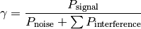
The test suite lte-downlink-sinr checks that the SINR calculation in downlink is performed correctly. The SINR in the downlink is calculated for each RB assigned to data transmissions by dividing the power of the intended signal from the considered eNB by the sum of the noise power plus all the transmissions on the same RB coming from other eNBs (the interference signals):
In general, different signals can be active during different periods
of time. We define a chunk as the time interval between any two
events of type either start or end of a waveform. In other words, a
chunk identifies a time interval during which the set of active
waveforms does not change. Let  be the generic chunk,
 its duration and
  its SINR,
calculated with the above equation. The calculation of the average
SINR
its SINR,
calculated with the above equation. The calculation of the average
SINR  to be used for CQI feedback reporting
uses the following formula:
to be used for CQI feedback reporting
uses the following formula:

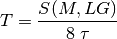
The test suite checks that the above calculation is performed
correctly in the simulator. The test vectors are obtained offline by
an Octave script that implements the above equation, and that
recreates a number of random transmitted signals and interference
signals that mimic a scenario where an UE is trying to decode a signal
from an eNB while facing interference from other eNBs. The test passes
if the calculated values are equal to the test vector within a
tolerance of  . The tolerance is meant to account for
the approximation errors typical of floating point arithmetic.
. The tolerance is meant to account for
the approximation errors typical of floating point arithmetic.
The test suite lte-uplink-sinr checks that the SINR calculation in uplink is performed correctly. This test suite is identical to lte-downlink-sinr described in the previous section, with the difference than both the signal and the interference now refer to transmissions by the UEs, and reception is performed by the eNB. This test suite recreates a number of random transmitted signals and interference signals to mimic a scenario where an eNB is trying to decode the signal from several UEs simultaneously (the ones in the cell of the eNB) while facing interference from other UEs (the ones belonging to other cells).
The test vectors are obtained by a dedicated Octave script. The test
passes if the calculated values are equal to the test vector within a
tolerance of which, as for the downlink SINR test,
deals with floating point arithmetic approximation issues.
The test suite lte-earfcn checks that the carrier frequency used by the LteSpectrumValueHelper class (which implements the LTE spectrum model) is done in compliance with [TS36101], where the E-UTRA Absolute Radio Frequency Channel Number (EARFCN) is defined. The test vector for this test suite comprises a set of EARFCN values and the corresponding carrier frequency calculated by hand following the specification of [TS36101]. The test passes if the carrier frequency returned by LteSpectrumValueHelper is the same as the known value for each element in the test vector.
The test suite lte-link-adaptation provides system tests recreating a scenario with a single eNB and a single UE. Different test cases are created corresponding to different SNR values perceived by the UE. The aim of the test is to check that in each test case the chosen MCS corresponds to some known reference values. These reference values are obtained by re-implementing in Octave (see src/lte/test/reference/lte_amc.m) the model described in Section Adaptive Modulation and Coding for the calculation of the spectral efficiency, and determining the corresponding MCS index by manually looking up the tables in [R1-081483]. The resulting test vector is represented in Figure Test vector for Adaptive Modulation and Coding.
The MCS which is used by the simulator is measured by obtaining the tracing output produced by the scheduler after 4ms (this is needed to account for the initial delay in CQI reporting). The SINR which is calcualted by the simulator is also obtained using the LteSinrChunkProcessor interface. The test passes if both the following conditions are satisfied:
- the SINR calculated by the simulator correspond to the SNR of the test vector within an absolute tolerance of
- the MCS index used by the simulator exactly corresponds to the one in the test vector.
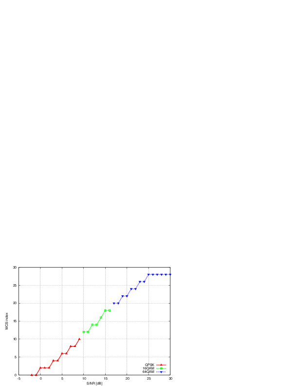
Test vector for Adaptive Modulation and Coding
The test suite lte-interference` provides system tests recreating an
inter-cell interference scenario with two eNBs, each having a single
UE attached to it and employing Adaptive Modulation and Coding both in
the downlink and in the uplink. The topology of the scenario
is depicted in Figure Topology for the inter-cell interference test. The
 parameter represents the distance of each UE to the eNB it
is attached to, whereas the
parameter represents the distance of each UE to the eNB it
is attached to, whereas the  parameter represent the
interferer distance. We note that the scenario topology is such that
the interferer distance is the same for uplink and downlink; still,
the actual interference power perceived will be different, because of
the different propagation loss in the uplink and downlink
bands. Different test cases are obtained by varying the
and parameters.
parameter represent the
interferer distance. We note that the scenario topology is such that
the interferer distance is the same for uplink and downlink; still,
the actual interference power perceived will be different, because of
the different propagation loss in the uplink and downlink
bands. Different test cases are obtained by varying the
and parameters.
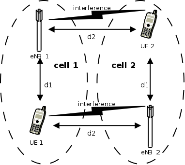
Topology for the inter-cell interference test
The test vectors are obtained by use of a dedicated octave script (available in src/lte/test/reference/lte_link_budget_interference.m), which does the link budget calculations (including interference) corresponding to the topology of each test case, and outputs the resulting SINR and spectral efficiency. The latter is then used to determine (using the same procedure adopted for Adaptive Modulation and Coding Tests. We note that the test vector contains separate values for uplink and downlink.
The test suite lte-rr-ff-mac-scheduler creates different test cases with a single eNB and several UEs, all having the same Radio Bearer specification. In each test case, the UEs see the same SINR from the eNB; different test cases are implemented by using different distance among UEs and the eNB (i.e., therefore having different SINR values) and different numbers of UEs. The test consists on checking that the obtained throughput performance is equal among users and matches a reference throughput value obtained according to the SINR perceived within a given tolerance.
The test vector is obtained according to the values of transport block
size reported in table 7.1.7.2.1-1 of [TS36213], considering an
equal distribution of the physical resource block among the users
using Resource Allocation Type 0 as defined in Section 7.1.6.1 of
[TS36213]. Let  be the TTI duration,
  be the
number of UEs,
be the
number of UEs,  the transmission bandwidth configuration in
number of RBs,
the transmission bandwidth configuration in
number of RBs,  the RBG size,
  the modulation and
coding scheme in use at the given SINR and
the modulation and
coding scheme in use at the given SINR and  be the
transport block size in bits as defined by 3GPP TS 36.213. We first
calculate the number
be the
transport block size in bits as defined by 3GPP TS 36.213. We first
calculate the number  of RBGs allocated to each user as

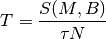
The reference throughput  in bit/s achieved by each UE is then calculated as
The test passes if the measured throughput matches with the reference throughput within a relative tolerance of 0.1. This tolerance is needed to account for the transient behavior at the beginning of the simulation (e.g., CQI feedback is only available after a few subframes) as well as for the accuracy of the estimator of the average throughput performance over the chosen simulation time (0.4s). This choice of the simulation time is justified by the need to follow the ns-3 guidelines of keeping the total execution time of the test suite low, in spite of the high number of test cases. In any case, we note that a lower value of the tolerance can be used when longer simulations are run.
In Figure fig-lenaThrTestCase1, the curves labeled “RR” represent the test values calculated for the RR scheduler test, as a function of the number of UEs and of the MCS index being used in each test case.
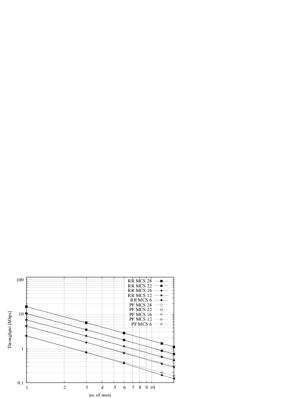
Test vectors for the RR and PF Scheduler in the downlink in a scenario where all UEs use the same MCS.
The test suite lte-pf-ff-mac-scheduler creates different test cases with a single eNB, using the Proportional Fair (PF) scheduler, and several UEs, all having the same Radio Bearer specification. The test cases are grouped in two categories in order to evaluate the performance both in terms of the adaptation to the channel condition and from a fairness perspective.
In the first category of test cases, the UEs are all placed at the
same distance from the eNB, and hence all placed in order to have the
same SINR. Different test cases are implemented by using a different
SINR value and a different number of UEs. The test consists on
checking that the obtained throughput performance matches with the
known reference throughput up to a given tolerance. The expected
behavior of the PF scheduler when all UEs have the same SNR is that
each UE should get an equal fraction of the throughput obtainable by a
single UE when using all the resources. We calculate the reference
throughput value by dividing the throughput achievable by a single UE
at the given SNR by the total number of UEs.
Let be the TTI duration, the transmission
bandwidth configuration in number of RBs, the modulation and
coding scheme in use at the given SINR and be the
transport block size as defined in [TS36213]. The reference
throughput in bit/s achieved by each UE is calculated as
The curves labeled “PF” in Figure fig-lenaThrTestCase1 represent the test values calculated for the PF scheduler tests of the first category, that we just described.
The second category of tests aims at verifying the fairness of the PF
scheduler in a more realistic simulation scenario where the UEs have a
different SINR (constant for the whole simulation). In these conditions, the PF
scheduler will give to each user a share of the system bandwidth that is
proportional to the capacity achievable by a single user alone considered its
SINR. In detail, let  be the modulation and coding scheme being used by
each UE (which is a deterministic function of the SINR of the UE, and is hence
known in this scenario). Based on the MCS, we determine the achievable
rate
be the modulation and coding scheme being used by
each UE (which is a deterministic function of the SINR of the UE, and is hence
known in this scenario). Based on the MCS, we determine the achievable
rate  for each user using the
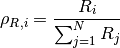
procedure described in Section~ref{sec:pfs}. We then define the
achievable rate ratio
for each user using the
procedure described in Section~ref{sec:pfs}. We then define the
achievable rate ratio  of each user as
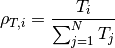
Let now be the throughput actually achieved by the UE , which
is obtained as part of the simulation output. We define the obtained throughput
ratio  of UE as
The test consists of checking that the following condition is verified:

if so, it means that the throughput obtained by each UE over the whole simulation matches with the steady-state throughput expected by the PF scheduler according to the theory. This test can be derived from [Holtzman2000] as follows. From Section 3 of [Holtzman2000], we know that

where  is a constant. By substituting the above into the
definition of given previously, we get
is a constant. By substituting the above into the
definition of given previously, we get
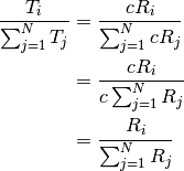
which is exactly the expression being used in the test.
Figure Throughput ratio evaluation for the PF scheduler in a scenario
where the UEs have MCS index presents the results obtained in a test case with
UEs  that are located at a distance from the base
station such that they will use respectively the MCS index
that are located at a distance from the base
station such that they will use respectively the MCS index 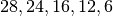 . From the figure, we note that, as expected, the obtained throughput is
proportional to the achievable rate. In other words, the PF scheduler assign
more resources to the users that use a higher MCS index.
. From the figure, we note that, as expected, the obtained throughput is
proportional to the achievable rate. In other words, the PF scheduler assign
more resources to the users that use a higher MCS index.
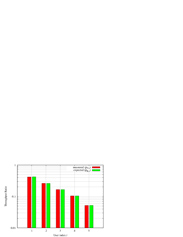
Throughput ratio evaluation for the PF scheduler in a scenario
where the UEs have MCS index 
Test suites lte-fdmt-ff-mac-scheduler and lte-tdmt-ff-mac-scheduler
create different test cases with a single eNB and several UEs, all having the same
Radio Bearer specification, using the Frequency Domain Maximum Throughput (FDMT)
scheduler and Time Domain Maximum Throughput (TDMT) scheduler respectively.
In other words, UEs are all placed at the
same distance from the eNB, and hence all placed in order to have the
same SNR. Different test cases are implemented by using a different
SNR values and a different number of UEs. The test consists on
checking that the obtained throughput performance matches with the
known reference throughput up to a given tolerance.The expected
behavior of both FDMT and TDMT scheduler when all UEs have the same SNR is that
scheduler allocates all RBGs to the first UE defined in script. This is because
the current FDMT and TDMT implementation always select the first UE to serve when there are
multiple UEs having the same SNR value. We calculate the reference
throughput value for first UE by the throughput achievable of a single UE
at the given SNR, while reference throughput value for other UEs by zero.
Let be the TTI duration, the transmission
bandwidth configuration in number of RBs, the modulation and
coding scheme in use at the given SNR and be the
transport block size as defined in [TS36.213]. The reference
throughput in bit/s achieved by each UE is calculated as
Test suites lte-tta-ff-mac-scheduler create different test cases with a single eNB and several UEs, all having the same Radio Bearer specification using TTA scheduler. Network topology and configurations in TTA test case are as the same as the test for MT scheduler. More complex test case needs to be developed to show the fairness feature of TTA scheduler.
Test suites lte-tdbet-ff-mac-scheduler and lte-fdbet-ff-mac-scheduler create different test cases with a single eNB and several UEs, all having the same Radio Bearer specification.
In the first test case of lte-tdbet-ff-mac-scheduler and lte-fdbet-ff-mac-scheduler, the UEs are all placed at the same distance from the eNB, and hence all placed in order to have the same SNR. Different test cases are implemented by using a different SNR value and a different number of UEs. The test consists on checking that the obtained throughput performance matches with the known reference throughput up to a given tolerance. In long term, the expected behavior of both TD-BET and FD-BET when all UEs have the same SNR is that each UE should get an equal throughput. However, the exact throughput value of TD-BET and FD-BET in this test case is not the same.
When all UEs have the same SNR, TD-BET can be seen as a specific case of PF where achievable rate equals to 1. Therefore, the throughput obtained by TD-BET is equal to that of PF. On the other hand, FD-BET performs very similar to the round robin (RR) scheduler in case of that all UEs have the same SNR and the number of UE( or RBG) is an integer multiple of the number of RBG( or UE). In this case, FD-BET always allocate the same number of RBGs to each UE. For example, if eNB has 12 RBGs and there are 6 UEs, then each UE will get 2 RBGs in each TTI. Or if eNB has 12 RBGs and there are 24 UEs, then each UE will get 2 RBGs per two TTIs. When the number of UE (RBG) is not an integer multiple of the number of RBG (UE), FD-BET will not follow the RR behavior because it will assigned different number of RBGs to some UEs, while the throughput of each UE is still the same.
The second category of tests aims at verifying the fairness of the both TD-BET and FD-BET schedulers in a more realistic simulation scenario where the UEs have a different SNR (constant for the whole simulation). In this case, both scheduler should give the same amount of averaged throughput to each user.
Specifically, for TD-BET, let  be the fraction of time allocated to user i in total simulation time,
 be the the full bandwidth achievable rate for user i and be the achieved throughput of
user i. Then we have:
be the the full bandwidth achievable rate for user i and be the achieved throughput of
user i. Then we have:

In TD-BET, the sum of for all user equals one. In long term, all UE has the same so that we replace
by . Then we have:
Test suites lte-fdtbfq-ff-mac-scheduler and lte-tdtbfq-ff-mac-scheduler create different test cases for testing three key features of TBFQ scheduler: traffic policing, fairness and traffic balance. Constant Bit Rate UDP traffic is used in both downlink and uplink in all test cases. The packet interval is set to 1ms to keep the RLC buffer non-empty. Different traffic rate is achieved by setting different packet size. Specifically, two classes of flows are created in the testsuites:
- Homogeneous flow: flows with the same token generation rate and packet arrival rate
- Heterogeneous flow: flows with different packet arrival rate, but with the same token generation rate
In test case 1 verifies traffic policing and fairness features for the scenario that all UEs are placed at the same distance from the eNB. In this case, all Ues have the same SNR value. Different test cases are implemented by using a different SNR value and a different number of UEs. Because each flow have the same traffic rate and token generation rate, TBFQ scheduler will guarantee the same throughput among UEs without the constraint of token generation rate. In addition, the exact value of UE throughput is depended on the total traffic rate:
- If total traffic rate <= maximum throughput, UE throughput = traffic rate
- If total traffic rate > maximum throughput, UE throughput = maximum throughput / N
Here, N is the number of UE connected to eNodeB. The maximum throughput in this case equals to the rate that all RBGs are assigned to one UE(e.g., when distance equals 0, maximum throughput is 2196000 byte/sec). When the traffic rate is smaller than max bandwidth, TBFQ can police the traffic by token generation rate so that the UE throughput equals its actual traffic rate (token generation rate is set to traffic generation rate); On the other hand, when total traffic rate is bigger than the max throughput, eNodeB cannot forward all traffic to UEs. Therefore, in each TTI, TBFQ will allocate all RBGs to one UE due to the large packets buffered in RLC buffer. When a UE is scheduled in current TTI, its token counter is decreased so that it will not be scheduled in the next TTI. Because each UE has the same traffic generation rate, TBFQ will serve each UE in turn and only serve one UE in each TTI (both in TD TBFQ and FD TBFQ). Therefore, the UE throughput in the second condition equals to the evenly share of maximum throughput.
Test case 2 verifies traffic policing and fairness features for the scenario that each UE is placed at the different distance from the eNB. In this case, each UE has the different SNR value. Similar to test case 1, UE throughput in test case 2 is also depended on the total traffic rate but with a different maximum throughput. Suppose all UEs have a high traffic load. Then the traffic will saturate the RLC buffer in eNodeB. In each TTI, after selecting one UE with highest metric, TBFQ will allocate all RBGs to this UE due to the large RLC buffer size. On the other hand, once RLC buffer is saturated, the total throughput of all UEs cannot increase any more. In addition, as we discussed in test case 1, for homogeneous flows which have the same t_i and r_i, each UE will achieve the same throughput in long term. Therefore, we can use the same method in TD BET to calculate the maximum throughput:

Here, is the maximum throughput. be the the full bandwidth achievable rate
for user i. is the number of UE.
When the totol traffic rate is bigger than , the UE throughput equals to  . Otherwise, UE throughput
equals to its traffic generation rate.
. Otherwise, UE throughput
equals to its traffic generation rate.
In test case 3, three flows with different traffic rate are created. Token generation rate for each flow is the same and equals to the average traffic rate of three flows. Because TBFQ use a shared token bank, tokens contributed by UE with lower traffic load can be utilized by UE with higher traffic load. In this way, TBFQ can guarantee the traffic rate for each flow. Although we use heterogeneous flow here, the calculation of maximum throughput is as same as that in test case 2. In calculation max throughput of test case 2, we assume that all UEs suffer high traffic load so that scheduler always assign all RBGs to one UE in each TTI. This assumes is also true in heterogeneous flow case. In other words, whether those flows have the same traffic rate and token generation rate, if their traffic rate is bigger enough, TBFQ performs as same as it in test case 2. Therefore, the maximum bandwidth in test case 3 is as same as it in test case 2.
In test case 3, in some flows, token generate rate does not equal to MBR, although all flows are CBR traffic. This is not accorded with our parameter setting rules. Actually, the traffic balance feature is used in VBR traffic. Because different UE’s peak rate may occur in different time, TBFQ use shared token bank to balance the traffic among those VBR traffics. Test case 3 use CBR traffic to verify this feature. But in the real simulation, it is recommended to set token generation rate to MBR.
Test suites lte-pss-ff-mac-scheduler create different test cases with a single eNB and several UEs. In all test cases, we select PFsch in FD scheduler. Same testing results can also be obtained by using CoItA scheduler. In addition, all test cases do not define nMux so that TD scheduler in PSS will always select half of total UE.
In the first class test case of lte-pss-ff-mac-scheduler, the UEs are all placed at the same distance from the eNB, and hence all placed in order to have the same SNR. Different test cases are implemented by using a different TBR for each UEs. In each test cases, all UEs have the same Target Bit Rate configured by GBR in EPS bear setting. The expected behavior of PSS is to guarantee that each UE’s throughput at least equals its TBR if the total flow rate is blow maximum throughput. Similar to TBFQ, the maximum throughput in this case equals to the rate that all RBGs are assigned to one UE. When the traffic rate is smaller than max bandwidth, the UE throughput equals its actual traffic rate; On the other hand, UE throughput equals to the evenly share of the maximum throughput.
In the first class of test cases, each UE has the same SNR. Therefore, the priority metric in PF scheduler will be
determined by past average throughput  because each UE has the same achievable throughput
 in PFsch or same
 ![CoI[k,n]](_images/math/d0da4949e2695aa7a6f0dedffc2fb42af9360d40.png) in CoItA. This means that PSS will performs like a
TD-BET which allocates all RBGs to one UE in each TTI. Then the maximum value of UE throughput equals to
the achievable rate that all RBGs are allocated to this UE.
in CoItA. This means that PSS will performs like a
TD-BET which allocates all RBGs to one UE in each TTI. Then the maximum value of UE throughput equals to
the achievable rate that all RBGs are allocated to this UE.
In the second class of test case of lte-pss-ff-mac-scheduler, the UEs are all placed at the same distance from the eNB, and hence all placed in order to have the same SNR. Different TBR values are assigned to each UE. There also exist an maximum throughput in this case. Once total traffic rate is bigger than this threshold, there will be some UEs that cannot achieve their TBR. Because there is no fading, subband CQIs for each RBGs frequency are the same. Therefore, in FD scheduler,in each TTI, priority metrics of UE for all RBGs are the same. This means that FD scheduler will always allocate all RBGs to one user. Therefore, in the maximum throughput case, PSS performs like a TD-BET. Then we have:
Here, is the maximum throughput. be the the full bandwidth achievable rate
for user i. is the number of UE.
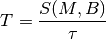
The aim of the system test is to verify the integration of the
BuildingPathlossModel with the lte module. The test exploits a set of
three pre calculated losses for generating the expected SINR at the
receiver counting the transmission and the noise powers. These SINR
values are compared with the results obtained from a LTE
simulation that uses the BuildingPathlossModel. The reference loss values are
calculated off-line with an Octave script
(/test/reference/lte_pathloss.m). Each test case passes if the
reference loss value is equal to the value calculated by the simulator
within a tolerance of  dB, which accouns for numerical
errors in the calculations.
dB, which accouns for numerical
errors in the calculations.
The test suite lte-phy-error-model generates different test cases for evaluating both data and control error models. For what concern the data, the test consists of nine test cases with single eNB and a various number of UEs, all having the same Radio Bearer specification. Each test is designed for evaluating the error rate perceived by a specific TB size in order to verify that it corresponds to the expected values according to the BLER generated for CB size analog to the TB size. This means that, for instance, the test will check that the performance of a TB of bits is analogous to the one of a a CB size of bits by collecting the performance of a user which has been forced the generation of a such TB size according to the distance to eNB. In order to significantly test the BER at MAC level, we modified the Adaptive Modulation and Coding (AMC) module, the LteAmc class, for making it less robust to channel conditions by adding a configurable BER parameter (called Ber in the ns3 attribute system) which enable the selection of the desired BER at MAC level when choosing the MCS to be used. In detail, the AMC module has been forced to select the AMC considering a BER of 0.01 (instead of the standard value equal to 0.00005). We note that, these values do not reflect actual BER since they come from an analytical bound which do not consider all the transmission chain aspects; therefore the resulted BER might be different.
The parameters of the nine test cases are reported in the following:
- 4 UEs placed 1800 meters far from the eNB, which implies the use of MCS 2 (SINR of -5.51 dB) and a TB of 256 bits, that in turns produce a BER of 0.33 (see point A in figure BLER for tests 1, 2, 3.).
- 2 UEs placed 1800 meters far from the eNB, which implies the use of MCS 2 (SINR of -5.51 dB) and a TB of 528 bits, that in turns produce a BER of 0.11 (see point B in figure BLER for tests 1, 2, 3.).
- 1 UE placed 1800 meters far from the eNB, which implies the use of MCS 2 (SINR of -5.51 dB) and a TB of 1088 bits, that in turns produce a BER of 0.02 (see point C in figure BLER for tests 1, 2, 3.).
- 1 UE placed 600 meters far from the eNB, which implies the use of MCS 12 (SINR of 4.43 dB) and a TB of 4800 bits, that in turns produce a BER of 0.3 (see point D in figure BLER for tests 4, 5.).
- 3 UEs placed 600 meters far from the eNB, which implies the use of MCS 12 (SINR of 4.43 dB) and a TB of 1632 bits, that in turns produce a BER of 0.55 (see point E in figure BLER for tests 4, 5.).
- 1 UE placed 470 meters far from the eNB, which implies the use of MCS 16 (SINR of 8.48 dB) and a TB of 7272 bits (segmented in 2 CBs of 3648 and 3584 bits), that in turns produce a BER of 0.14, since each CB has CBLER equal to 0.075 (see point F in figure BLER for test 6.).
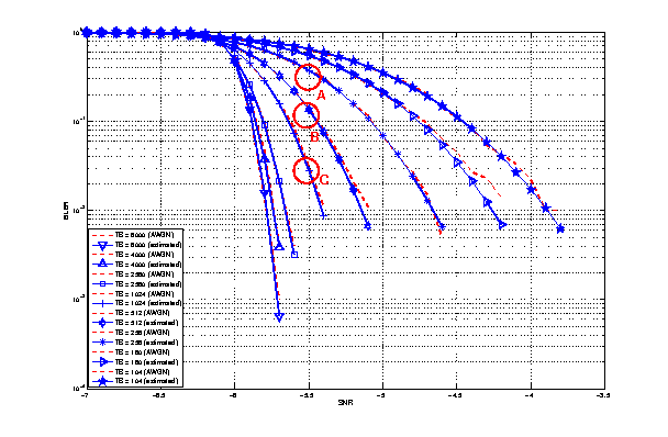
BLER for tests 1, 2, 3.
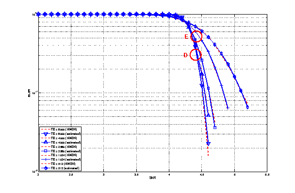
BLER for tests 4, 5.
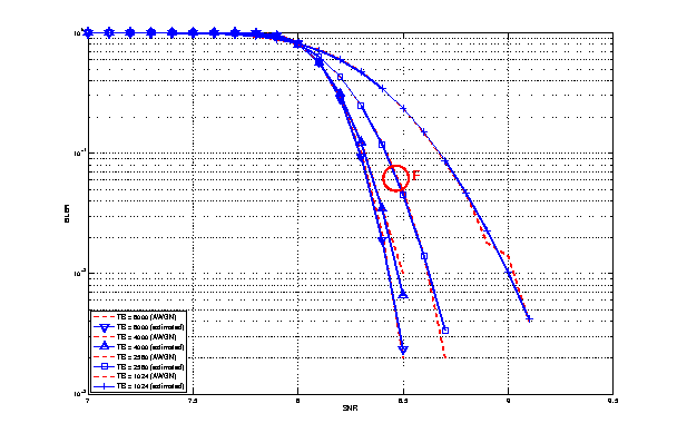
BLER for test 6.
The test verifies that in each case the expected number of packets received correct corresponds to a Bernoulli distribution with a confidence interval of 95%, where the probability of success in each trail is  and
and  is the total number of packet sent.
The error model of PCFICH-PDDCH channels consists of 4 test cases with a single UE and several eNBs, where the UE is connected to only one eNB in order to have the remaining acting as interfering ones. The errors on data are disabled in order to verify only the ones due to erroneous decodification of PCFICH-PDCCH. The test verifies that the error on the data received respects the decodification error probability of the PCFICH-PDCCH with a tolerance of 0.1 due to the errors that might be produced in quantizing the MI and the error curve. As before, the system has been forced on working in a less conservative fashion in the AMC module for appreciating the results in border situations. The parameters of the 4 tests cases are reported in the following:
- 2 eNBs placed 1078 meters far from the UE, which implies a SINR of -2.00 dB and a TB of 217 bits, that in turns produce a BER of 0.007.
- 3 eNBs placed 1078 meters far from the UE, which implies a SINR of -4.00 dB and a TB of 217 bits, that in turns produce a BER of 0.045.
- 4 eNBs placed 1078 meters far from the UE, which implies a SINR of -6.00 dB and a TB of 133 bits, that in turns produce a BER of 0.206.
- 5 eNBs placed 1078 meters far from the UE, which implies a SINR of -7.00 dB and a TB of 81 bits, that in turns produce a BER of 0.343.
The test suite lte-mimo aims at verifying both the effect of the gain considered for each Transmission Mode on the system performance and the Transmission Mode switching through the scheduler interface. The test consists on checking whether the amount of bytes received during a certain window of time (0.1 seconds in our case) corresponds to the expected ones according to the values of transport block size reported in table 7.1.7.2.1-1 of [TS36213], similarly to what done for the tests of the schedulers.
The test is performed both for Round Robin and Proportional Fair schedulers. The test passes if the measured throughput matches with the reference throughput within a relative tolerance of 0.1. This tolerance is needed to account for the transient behavior at the beginning of the simulation and the transition phase between the Transmission Modes.
The test suite lte-antenna checks that the AntennaModel integrated
with the LTE model works correctly. This test suite recreates a
simulation scenario with one eNB node at coordinates (0,0,0) and one
UE node at coordinates (x,y,0). The eNB node is configured with an
CosineAntennaModel having given orientation and beamwidth. The UE
instead uses the default IsotropicAntennaModel. The test
checks that the received power both in uplink and downlink account for
the correct value of the antenna gain, which is determined
offline; this is implemented by comparing the uplink and downlink SINR
and checking that both match with the reference value up to a
tolerance of  which accounts for numerical errors.
Different test cases are provided by varying the x and y coordinates
of the UE, and the beamwidth and the orientation of the antenna of
the eNB.
which accounts for numerical errors.
Different test cases are provided by varying the x and y coordinates
of the UE, and the beamwidth and the orientation of the antenna of
the eNB.
Two test suites lte-rlc-um-transmitter and lte-rlc-am-transmitter check that the UM RLC and the AM RLC implementation work correctly. Both these suites work by testing RLC instances connected to special test entities that play the role of the MAC and of the PDCP, implementing respectively the LteMacSapProvider and LteRlcSapUser interfaces. Different test cases (i.e., input test vector consisting of series of primitive calls by the MAC and the PDCP) are provided that check the behavior in the following cases:
- one SDU, one PDU: the MAC notifies a TX opportunity causes the creation of a PDU which exactly contains a whole SDU
- segmentation: the MAC notifies multiple TX opportunities that are smaller than the SDU size stored in the transmission buffer, which is then to be fragmented and hence multiple PDUs are generated;
- concatenation: the MAC notifies a TX opportunity that is bigger than the SDU, hence multiple SDUs are concatenated in the same PDU
- buffer status report: a series of new SDUs notifications by the PDCP is inteleaved with a series of TX opportunity notification in order to verify that the buffer status report procedure is correct.
In all these cases, an output test vector is determine manually from knowledge of the input test vector and knowledge of the expected behavior. These test vector are specialized for UM RLC and AM RLC due to their different behavior. Each test case passes if the sequence of primitives triggered by the RLC instance being tested is exacly equal to the output test vector. In particular, for each PDU transmitted by the RLC instance, both the size and the content of the PDU are verified to check for an exact match with the test vector.
The unit test suite epc-gtpu checks that the encoding and decoding of the GTP-U header is done correctly. The test fills in a header with a set of known values, adds the header to a packet, and then removes the header from the packet. The test fails if, upon removing, any of the fields in the GTP-U header is not decoded correctly. This is detected by comparing the decoded value from the known value.
Two test suites (epc-s1u-uplink and epc-s1u-downlink) make sure that the S1-U interface implementation works correctly in isolation. This is achieved by creating a set of simulation scenarios where the EPC model alone is used, without the LTE model (i.e., without the LTE radio protocol stack, which is replaced by simple CSMA devices). This checks that the interoperation between multiple EpcEnbApplication instances in multiple eNBs and the EpcSgwPgwApplication instance in the SGW/PGW node works correctly in a variety of scenarios, with varying numbers of end users (nodes with a CSMA device installed), eNBs, and different traffic patterns (packet sizes and number of total packets). Each test case works by injecting the chosen traffic pattern in the network (at the considered UE or at the remote host for in the uplink or the downlink test suite respectively) and checking that at the receiver (the remote host or each considered UE, respectively) that exactly the same traffic patterns is received. If any mismatch in the transmitted and received traffic pattern is detected for any UE, the test fails.
The test suite epc-tft-classifier checks in isolation that the behavior of the EpcTftClassifier class is correct. This is performed by creating different classifier instances where different TFT instances are activated, and testing for each classifier that an heterogeneous set of packets (including IP and TCP/UDP headers) is classified correctly. Several test cases are provided that check the different matching aspects of a TFT (e.g. local/remote IP address, local/remote port) both for uplink and downlink traffic. Each test case corresponds to a specific packet and a specific classifier instance with a given set of TFTs. The test case passes if the bearer identifier returned by the classifier exactly matches with the one that is expected for the considered packet.
The test suite lte-epc-e2e-data ensures the correct end-to-end functionality of the LTE-EPC data plane. For each test case in this suite, a complete LTE-EPC simulation scenario is created with the following characteristics:
- a given number of eNBs
- for each eNB, a given number of UEs
- for each UE, a given number of active EPS bearers
- for each active EPS bearer, a given traffic pattern (number of UDP packets to be transmitted and packet size)
Each test is executed by transmitting the given traffic pattern both in the uplink and in the downlink, at subsequent time intervals. The test passes if all the following conditions are satisfied:
- for each active EPS bearer, the transmitted and received traffic pattern (respectively at the UE and the remote host for uplink, and vice versa for downlink) is exactly the same
- for each active EPS bearer and each direction (uplink or downlink), exactly the expected number of packet flows over the corresponding RadioBearer instance