
|
A Discrete-Event Network Simulator
|
Models |
|
|
A Discrete-Event Network Simulator
|
Models |
The ns-3 propagation module defines two generic interfaces, namely PropagationLossModel and PropagationDelayModel, for the modeling of respectively propagation loss and propagation delay.
Propagation loss models calculate the Rx signal power considering the Tx signal power and the mutual Rx and Tx antennas positions.
A propagation loss model can be “chained” to another one, making a list. The final Rx power takes into account all the chained models. In this way one can use a slow fading and a fast fading model (for example), or model separately different fading effects.
The following propagation delay models are implemented:
Other models could be available thanks to other modules, e.g., the building module.
Each of the available propagation loss models of ns-3 is explained in one of the following subsections.
This model implements the Friis propagation loss model. This model was first described in [friis]. The original equation was described as:

with the following equation for the case of an isotropic antenna with no heat loss:

The final equation becomes:

Modern extensions to this original equation are:
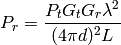
With:
: transmission power (W)
: reception power (W)
: transmission gain (unit-less)
: reception gain (unit-less)
: wavelength (m)
: distance (m)
: system loss (unit-less)
In the implementation, is calculated as
 , where
  m/s is the speed of light in
vacuum, and
m/s is the speed of light in
vacuum, and  is the frequency in Hz which can be configured by
the user via the Frequency attribute.
is the frequency in Hz which can be configured by
the user via the Frequency attribute.
The Friis model is valid only for propagation in free space within
the so-called far field region, which can be considered
approximately as the region for  .
The model will still return a value for , as
doing so (rather than triggering a fatal error) is practical for
many simulation scenarios. However, we stress that the values
obtained in such conditions shall not be considered realistic.
.
The model will still return a value for , as
doing so (rather than triggering a fatal error) is practical for
many simulation scenarios. However, we stress that the values
obtained in such conditions shall not be considered realistic.
Related with this issue, we note that the Friis formula is
undefined for  , and results in
 for
for  .
.
Both these conditions occur outside of the far field region, so in
principle the Friis model shall not be used in these conditions.
In practice, however, Friis is often used in scenarios where accurate
propagation modeling is not deemed important, and values of
can occur.
To allow practical use of the model in such
scenarios, we have to 1) return some value for , and
2) avoid large discontinuities in propagation loss values (which
could lead to artifacts such as bogus capture effects which are
much worse than inaccurate propagation loss values). The two issues
are conflicting, as, according to the Friis formula,
 ;
so if, for , we use a fixed loss value, we end up with an infinitely large
discontinuity, which as we discussed can cause undesirable
simulation artifacts.
;
so if, for , we use a fixed loss value, we end up with an infinitely large
discontinuity, which as we discussed can cause undesirable
simulation artifacts.
To avoid these artifact, this implementation of the Friis model
provides an attribute called MinLoss which allows to specify the
minimum total loss (in dB) returned by the model. This is used in
such a way that
continuously increases for  , until
MinLoss is reached, and then stay constant; this allow to
return a value for and at the same time avoid
discontinuities. The model won’t be much realistic, but at least
the simulation artifacts discussed before are avoided. The default value of
MinLoss is 0 dB, which means that by default the model will return
, until
MinLoss is reached, and then stay constant; this allow to
return a value for and at the same time avoid
discontinuities. The model won’t be much realistic, but at least
the simulation artifacts discussed before are avoided. The default value of
MinLoss is 0 dB, which means that by default the model will return
 for
for  .
We note that this value of is outside of the far field
region, hence the validity of the model in the far field region is
not affected.
.
We note that this value of is outside of the far field
region, hence the validity of the model in the far field region is
not affected.
This model implements a Two-Ray Ground propagation loss model ported from NS2
The Two-ray ground reflection model uses the formula
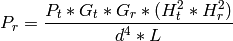
The original equation in Rappaport’s book assumes  .
To be consistent with the free space equation, is added here.
.
To be consistent with the free space equation, is added here.
 and
and  are set at the respective nodes
  coordinate plus a model parameter
set via SetHeightAboveZ.
coordinate plus a model parameter
set via SetHeightAboveZ.
The two-ray model does not give a good result for short distances, due to the oscillation caused by constructive and destructive combination of the two rays. Instead the Friis free-space model is used for small distances.
The crossover distance, below which Friis is used, is calculated as follows:
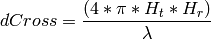
In the implementation, is calculated as
, where m/s is the speed of light in
vacuum, and is the frequency in Hz which can be configured by
the user via the Frequency attribute.
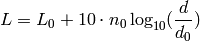
This model implements a log distance propagation model.
The reception power is calculated with a so-called log-distance propagation model:
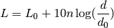
where:
: the path loss distance exponent
: reference distance (m)
: path loss at reference distance (dB)
When the path loss is requested at a distance smaller than the reference distance, the tx power is returned.
This model implements a log distance path loss propagation model with three distance fields. This model is the same as ns3::LogDistancePropagationLossModel except that it has three distance fields: near, middle and far with different exponents.
Within each field the reception power is calculated using the log-distance propagation equation:
Each field begins where the previous ends and all together form a continuous function.
There are three valid distance fields: near, middle, far. Actually four: the first from 0 to the reference distance is invalid and returns txPowerDbm.

Complete formula for the path loss in dB:
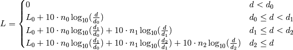
where:
: three distance fields (m)
: path loss distance exponent for each field (unitless)
When the path loss is requested at a distance smaller than the reference
distance , the tx power (with no path loss) is returned. The
reference distance defaults to 1m and reference loss defaults to
FriisPropagationLossModel with 5.15 GHz and is thus = 46.67 dB.
The propagation loss is totally random, and it changes each time the model is called. As a consequence, all the packets (even those between two fixed nodes) experience a random propagation loss.
This propagation loss model implements Nakagami-m fast fading propagation loss model.
The Nakagami-m distribution is applied to the power level. The probability density function is defined as

with  the fading depth parameter and
  the average received power.
It is implemented by either a GammaRandomVariable or a ErlangRandomVariable random variable.
Like in :cpp:class:ThreeLogDistancePropagationLossModel`, the parameter is varied
over three distance fields:

For  the Nakagami-m distribution equals the Rayleigh distribution. Thus
this model also implements Rayleigh distribution based fast fading.
the Nakagami-m distribution equals the Rayleigh distribution. Thus
this model also implements Rayleigh distribution based fast fading.
This model sets a constant received power level independent of the transmit power.
The received power is constant independent of the transmit power; the user must set received power level. Note that if this loss model is chained to other loss models, it should be the first loss model in the chain. Else it will disregard the losses computed by loss models that precede it in the chain.
The propagation loss is fixed for each pair of nodes and doesn’t depend on their actual positions. This model shoud be useful for synthetic tests. Note that by default the propagation loss is assumed to be symmetric.
This propagation loss depends only on the distance (range) between transmitter and receiver.
The single MaxRange attribute (units of meters) determines path loss. Receivers at or within MaxRange meters receive the transmission at the transmit power level. Receivers beyond MaxRange receive at power -1000 dBm (effectively zero).
This model is used to model open area pathloss for long distance (i.e., > 1 Km). In order to include all the possible frequencies usable by LTE we need to consider several variants of the well known Okumura Hata model. In fact, the original Okumura Hata model [hata] is designed for frequencies ranging from 150 MHz to 1500 MHz, the COST231 [cost231] extends it for the frequency range from 1500 MHz to 2000 MHz. Another important aspect is the scenarios considered by the models, in fact the all models are originally designed for urban scenario and then only the standard one and the COST231 are extended to suburban, while only the standard one has been extended to open areas. Therefore, the model cannot cover all scenarios at all frequencies. In the following we detail the models adopted.
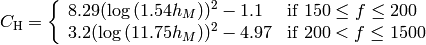
The pathloss expression of the COST231 OH is:

where

and
: eNB height above the ground [m]
: UE height above the ground [m]
: is a logarithm in base 10 (this for the whole document)
This model is only for urban scenarios.
The pathloss expression of the standard OH in urban area is:

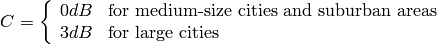
where for small or medium sized city

and for large cities
There extension for the standard OH in suburban is
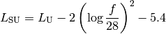
where
: pathloss in urban areas
The extension for the standard OH in open area is

The literature lacks of extensions of the COST231 to open area (for suburban it seems that we can just impose C = 0); therefore we consider it a special case fo the suburban one.
This model is designed for Line-of-Sight (LoS) short range outdoor communication in the frequency range 300 MHz to 100 GHz. This model provides an upper and lower bound respectively according to the following formulas
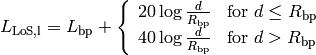
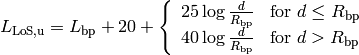
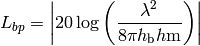
where the breakpoint distance is given by
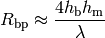
and the above parameters are
: UE height above the ground [m]
and  is the value for the basic transmission loss at the break point, defined as:
The value used by the simulator is the average one for modeling the median pathloss.
This model is designed for Non-Line-of-Sight (LoS) short range outdoor communication over rooftops in the frequency range 300 MHz to 100 GHz. This model includes several scenario-dependent parameters, such as average street width, orientation, etc. It is advised to set the values of these parameters manually (using the ns-3 attribute system) according to the desired scenario.
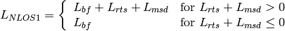
In detail, the model is based on [walfisch] and [ikegami], where the loss is expressed
as the sum of free-space loss ( ), the diffraction loss from rooftop to
street (
), the diffraction loss from rooftop to
street ( ) and the reduction due to multiple screen diffraction past
rows of building (
) and the reduction due to multiple screen diffraction past
rows of building ( ). The formula is:
The free-space loss is given by:

where:
) [m]
The term takes into account the width of the street and its orientation, according to the formulas
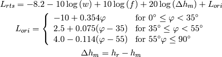
where:
: is the height of the rooftop [m]
: is the height of the mobile [m]
: is the street orientation with respect to the direct path (degrees)
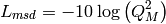
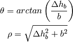
The multiple screen diffraction loss depends on the BS antenna height relative to the building height and on the incidence angle. The former is selected as the higher antenna in the communication link. Regarding the latter, the “settled field distance” is used for select the proper model; its value is given by

with
Therefore, in case of  (where l is the distance over which the building extend),
it can be evaluated according to
(where l is the distance over which the building extend),
it can be evaluated according to
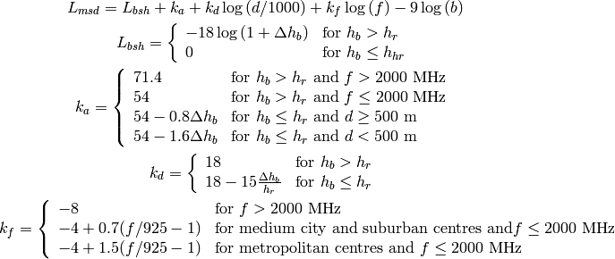
Alternatively, in case of  , the formula is:
where
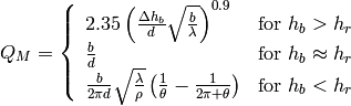
where:
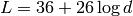
This is the empirical model for the pathloss at 2600 MHz for urban areas which is described in [kun2600mhz].
The model is as follows. Let be the distance between the transmitter and the receiver
in meters; the pathloss in dB is calculated as:
The following propagation delay models are implemented:
In this model, the signal travels with constant speed. The delay is calculated according with the trasmitter and receiver positions. The Euclidean distance between the Tx and Rx antennas is used. Beware that, according to this model, the Earth is flat.
The propagation delay is totally random, and it changes each time the model is called. All the packets (even those between two fixed nodes) experience a random delay. As a consequence, the packets order is not preserved.
| [friis] | Friis, H.T., “A Note on a Simple Transmission Formula,” Proceedings of the IRE , vol.34, no.5, pp.254,256, May 1946 |
| [hata] | M.Hata, “Empirical formula for propagation loss in land mobile radio services”, IEEE Trans. on Vehicular Technology, vol. 29, pp. 317-325, 1980 |
| [cost231] | “Digital Mobile Radio: COST 231 View on the Evolution Towards 3rd Generation Systems”, Commission of the European Communities, L-2920, Luxembourg, 1989 |
| [walfisch] | J.Walfisch and H.L. Bertoni, “A Theoretical model of UHF propagation in urban environments,” in IEEE Trans. Antennas Propagat., vol.36, 1988, pp.1788- 1796 |
| [ikegami] | F.Ikegami, T.Takeuchi, and S.Yoshida, “Theoretical prediction of mean field strength for Urban Mobile Radio”, in IEEE Trans. Antennas Propagat., Vol.39, No.3, 1991 |
| [kun2600mhz] | Sun Kun, Wang Ping, Li Yingze, “Path loss models for suburban scenario at 2.3GHz, 2.6GHz and 3.5GHz”, in Proc. of the 8th International Symposium on Antennas, Propagation and EM Theory (ISAPE), Kunming, China, Nov 2008. |