|
A Discrete-Event Network Simulator
|
Models |
|
|
A Discrete-Event Network Simulator
|
Models |
The main objective of the profiling carried out is to assess the simulator performance on a broad set of scenarios. This evaluation provides reference values for simulation running times and memory consumption figures. It also helps to identify potential performance improvements and to check for scalability problems when increasing the number of eNodeB and UEs attached to those.
In the following sections, a detailed description of the general profiling framework employed to perform the study is introduced. It also includes details on the main performed tests and its results evaluation.
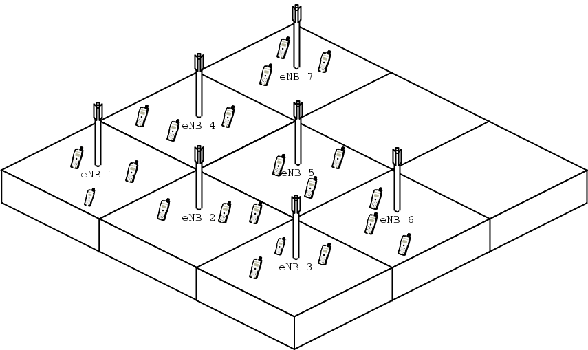
The simulation script used for all the E-UTRAN results showed in this documentation is located at src/lte/examples/lena-profiling.cc. It uses the complete PHY and MAC UE/eNodeB implementation with a simplified RLC implementation on top. This script generates a squared grid topology, placing a eNodeB at the centre of each square. UEs attached to this node are scattered randomly across the square (using a random uniform distribution along X and Y axis). If BuildingPropagationModel is used, the squares are replaced by rooms. To generate the UL and DL traffic, the RLC implementation always report data to be transfered.
E-UTRAN
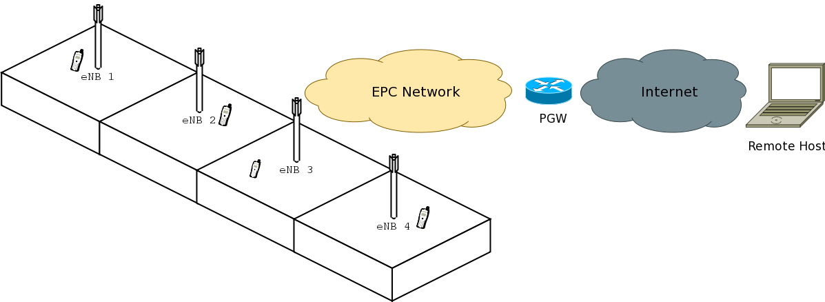
For the EPC results, the script is src/lte/examples/lena-simple-epc.cc. It uses a complete E-UTRAN implementation (PHY+MAC+RLC/UM+PDCP) and the most relevant EPC user plane entities the PGW and SGW, including GTP-U tunneling. This script generates a given number of eNodeBs, distributed across a line and attaches a single UE to every eNodeB. It also creates an EPC network and an external host connected to it through the Internet. Each UE sends and receives data to and from the remote host. In addition, each UE is also sending data to the UE camped in the adjacent eNodeB.
Propagation Model
RLC and MAC traces are enabled for all UEs and all eNodeBs and those traces are written to disk directly. The MAC scheduler used is round robin.
The lena-profiling simulation script accepts the following input parameters:
- simTime: time to simulate (in seconds)
- nUe: number of UEs attached to each eNodeB
- nEnb: number of eNodeB composing the grid per floor
- nFloors: number of floors, 0 for Friis propagation model (no walls), 1 or greater for Building propagation model generating a nFloors-storey building.
- traceDirectory: destination directory where simulation traces will be stored
The lena-simple-epc script accepts those other parameters:
- simTime: time to simulate (in seconds)
- numberOfNodes: number of eNodeB + UE pairs created
Running time is measured using default Linux shell command time. This command counts how much user time the execution of a program takes.
To simplify the process of running the profiling script for a wide range of values and collecting its timing data, a simple Perl script to automate the complete process is provided. It is placed in src/lte/test/lte-test-run-time.pl for lena-profiling and in src/lte/epc-test-run-time.pl for lena-simple-epc. It simply runs a batch of simulations with a range of parameters and stores the timing results in a CSV file called lteTimes.csv and epcTimes.csv respectively. The range of values each parameter sweeps can be modified editing the corresponding script.
For installing the modules, simply use the following command:
perl -MCPAN -e 'install moduleName'
To plot the results obtained from running the Perl scripts, two gnuplot scripts are provided, in src/lte/test/lte-test-run-plot and src/lte/test/epc-test-run-plot. Most of the plots available in this documentation can be reproduced with those, typing the commands gnuplot < src/lte/test/lte-test-run-plot and gnuplot < src/lte/test/epc-test-run-plot.
All timing tests had been run in a Intel Pentium IV 3.00 GHz machine with 512 Mb of RAM memory running Fedora Core 10 with a 2.6.27.41-170.2.117 kernel, storing the traces directly to the hard disk.
Also, as a reference configuration, the build has been configured static and optimized. The exact waf command issued is:
CXXFLAGS="-O3 -w" ./waf -d optimized configure --enable-static --enable-examples --enable-modules=lte
The following results and figures had been obtained with LENA changeset 2c5b0d697717.
This scenario, evaluates the running time for a fixed simulation time (10s) and Friis propagation mode increasing the number of UEs attached to each eNodeB and the number of planted eNodeBs in the scenario.
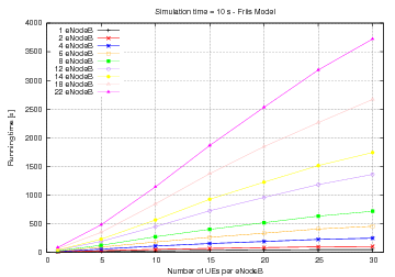
Running time
The figure shows the expected behaviour, since it increases linearly respect the number of UEs per eNodeB and quadratically respect the total number of eNodeBs.
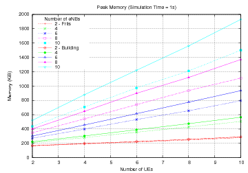
The objective of this scenario is to evaluate the impact of the propagation model complexity in the overall run time figures. Therefore, the same scenario is simulated twice: once using the more simple Friis model, once with the more complex Building model. The rest of the parameters (e.g. number of eNodeB and of UE attached per eNodeB) were mantained. The timing results for both models are compared in the following figure.
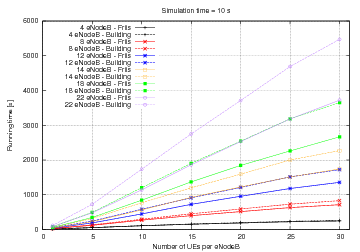
Propagation Model
In this situation, results are also coherent with what is expected. The more complex the model, the higher the running time. Moreover, as the number of computed path losses increases (i.e. more UEs per eNodeB or more eNodeBs) the extra complexity of the propagation model drives the running time figures further apart.
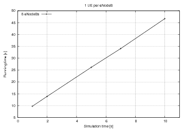
In this scenario, for a fixed set of UEs per eNodeB, different simulation times had been run. As the simulation time increases, running time should also increase linearly, i.e. for a given scenario, simulate four seconds should take twice times what it takes to simulate two seconds. The slope of this line is a function of the complexity of the scenario: the more eNodeB / UEs placed, the higher the slope of the line.
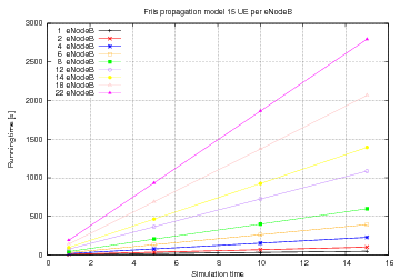
Simulation time
The following results and figures had been obtained with LENA changeset e8b3ccdf6673. The rationale behind the two scenarios profiled on this section is the same than for the E-UTRA part.
Running time evolution is quadratic since we increase at the same time the number of eNodeB and the number of UEs.
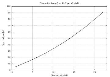
Running time
To estimate the additional complexity of the upper LTE Radio Protocol Stack model and the EPC model, we compare two scenarios using the simplified E-UTRAN version (using only PHY, MAC and the simplified RLC/SM, with no EPC and no ns-3 applications) against the complete E-UTRAN + EPC (with UM RLC, PDCP, end-to-end IP networking and regular ns-3 applications). Both configuration have been tested with the same number of UEs per eNodeB, the same number of eNodeBs, and approximately the same volume of transmitted data (an exact match was not possible due to the different ways in which packets are generated in the two configurations).
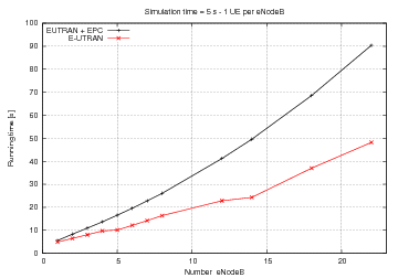
EPC E-UTRAN running time
From the figure, it is evident that the additional complexity of using the upper LTE stack plus the EPC model translates approximately into a doubling of the execution time of the simulations. We believe that, considered all the new features that have been added, this figure is acceptable.
Finally, again the linearity of the running time as the simulation time increases gets validated through a set of experiments, as the following figure shows.
Simulation time