| [ < ] | [ > ] | [ << ] | [ Up ] | [ >> ] | [Top] | [Contents] | [Index] | [ ? ] |
Let’s do an example taken from one of the best-known books on TCP around.
“TCP/IP Illustrated, Volume 1: The Protocols,” by W. Richard Stevens is a
classic. I just flipped the book open and ran across a nice plot of both the
congestion window and sequence numbers versus time on page 366. Stevens calls
this, “Figure 21.10. Value of cwnd and send sequence number while data is being
transmitted.” Let’s just recreate the cwnd part of that plot in ns-3
using the tracing system and gnuplot.
| [ < ] | [ > ] | [ << ] | [ Up ] | [ >> ] | [Top] | [Contents] | [Index] | [ ? ] |
The first thing to think about is how we want to get the data out. What is it
that we need to trace? The first thing to do is to consult “The list of all
trace sources” to see what we have to work with. Recall that this is found
in the ns-3 Doxygen in the “Core” Module section. If you scroll
through the list, you will eventually find:
  ns3::TcpSocketImpl
  CongestionWindow: The TCP connection's congestion window
It turns out that the ns-3 TCP implementation lives (mostly) in the
file src/internet-stack/tcp-socket-impl.cc. If you don’t know this a
priori, you can use the recursive grep trick:
find . -name '*.cc' | xargs grep -i tcp
You will find page after page of instances of tcp pointing you to that file.
If you open src/internet-stack/tcp-socket-impl.cc in your favorite
editor, you will see right up at the top of the file, the following declarations:
  TypeId
  TcpSocketImpl::GetTypeId ()
  {
    static TypeId tid = TypeId(``ns3::TcpSocketImpl'')
      .SetParent<TcpSocket> ()
      .AddTraceSource (``CongestionWindow'',
                       ``The TCP connection's congestion window'',
                       MakeTraceSourceAccessor (&TcpSocketImpl::m_cWnd))
      ;
    return tid;
  }
This should tell you to look for the declaration of m_cWnd in the header
file src/internet-stack/tcp-socket-impl.h. If you open this file in your
favorite editor, you will find:
TracedValue<uint32_t> m_cWnd; //Congestion window
You should now understand this code completely. If we have a pointer to the
TcpSocketImpl, we can TraceConnect to the “CongestionWindow” trace
source if we provide an appropriate callback target. This is the same kind of
trace source that we saw in the simple example at the start of this section,
except that we are talking about uint32_t instead of int32_t.
We now know that we need to provide a callback that returns void and takes
two uint32_t parameters, the first being the old value and the second
being the new value:
  void
  CwndTrace (uint32_t oldValue, uint32_t newValue)
  {
    ...
  }
| [ < ] | [ > ] | [ << ] | [ Up ] | [ >> ] | [Top] | [Contents] | [Index] | [ ? ] |
It’s always best to try and find working code laying around that you can modify, rather than starting from scratch. So the first order of business now is to find some code that already hooks the “CongestionWindow” trace source and see if we can modify it. As usual, grep is your friend:
find . -name '*.cc' | xargs grep CongestionWindow
This will point out a couple of promising candidates:
examples/tcp/tcp-large-transfer.cc and
src/test/ns3tcp/ns3tcp-cwnd-test-suite.cc.
We haven’t visited any of the test code yet, so let’s take a look there. You
will typically find that test code is fairly minimal, so this is probably a
very good bet. Open src/test/ns3tcp/ns3tcp-cwnd-test-suite.cc in your
favorite editor and search for “CongestionWindow”. You will find,
  ns3TcpSocket->TraceConnectWithoutContext (``CongestionWindow'',
    MakeCallback (&Ns3TcpCwndTestCase1::CwndChange, this));
This should look very familiar to you. We mentioned above that if we had a
pointer to the TcpSocketImpl, we could TraceConnect to the
“CongestionWindow” trace source. That’s exactly what we have here; so it
turns out that this line of code does exactly what we want. Let’s go ahead
and extract the code we need from this function
(Ns3TcpCwndTestCase1::DoRun (void)). If you look at this function,
you will find that it looks just like an ns-3 script. It turns out that
is exactly what it is. It is a script run by the test framework, so we can just
pull it out and wrap it in main instead of in DoRun. Rather than
walk through this, step, by step, we have provided the file that results from
porting this test back to a native ns-3 script –
examples/tutorial/fifth.cc.
| [ < ] | [ > ] | [ << ] | [ Up ] | [ >> ] | [Top] | [Contents] | [Index] | [ ? ] |
The fifth.cc example demonstrates an extremely important rule that you
must understand before using any kind of Attribute: you must ensure
that the target of a Config command exists before trying to use it.
This is no different than saying an object must be instantiated before trying
to call it. Although this may seem obvious when stated this way, it does
trip up many people trying to use the system for the first time.
Let’s return to basics for a moment. There are three basic time periods that
exist in any ns-3 script. The first time period is sometimes called
“Configuration Time” or “Setup Time,” and is in force during the period
when the main function of your script is running, but before
Simulator::Run is called. The second time period is sometimes called
“Simulation Time” and is in force during the time period when
Simulator::Run is actively executing its events. After it completes
executing the simulation, Simulator::Run will return control back to
the main function. When this happens, the script enters what can be
called “Teardown Time,” which is when the structures and objects created
during setup and taken apart and released.
Perhaps the most common mistake made in trying to use the tracing system is
assuming that entities constructed dynamically during simulation time are
available during configuration time. In particular, an ns-3
Socket is a dynamic object often created by Applications to
communicate between Nodes. An ns-3 Application
always has a “Start Time” and a “Stop Time” associated with it. In the
vast majority of cases, an Application will not attempt to create
a dynamic object until its StartApplication method is called at some
“Start Time”. This is to ensure that the simulation is completely
configured before the app tries to do anything (what would happen if it tried
to connect to a node that didn’t exist yet during configuration time). The
answer to this issue is to 1) create a simulator event that is run after the
dynamic object is created and hook the trace when that event is executed; or
2) create the dynamic object at configuration time, hook it then, and give
the object to the system to use during simulation time. We took the second
approach in the fifth.cc example. This decision required us to create
the MyApp Application, the entire purpose of which is to take
a Socket as a parameter.
| [ < ] | [ > ] | [ << ] | [ Up ] | [ >> ] | [Top] | [Contents] | [Index] | [ ? ] |
Now, let’s take a look at the example program we constructed by dissecting
the congestion window test. Open examples/tutorial/fifth.cc in your
favorite editor. You should see some familiar looking code:
  /* -*- Mode:C++; c-file-style:''gnu''; indent-tabs-mode:nil; -*- */
  /*
   * This program is free software; you can redistribute it and/or modify
   * it under the terms of the GNU General Public License version 2 as
   * published by the Free Software Foundation;
   *
   * This program is distributed in the hope that it will be useful,
   * but WITHOUT ANY WARRANTY; without even the implied warranty of
   * MERCHANTABILITY or FITNESS FOR A PARTICULAR PURPOSE.  See the
   * GNU General Public License for more details.
   *
   * You should have received a copy of the GNU General Public License
   * along with this program; if not, write to the Free Software
   * Foundation, Include., 59 Temple Place, Suite 330, Boston, MA  02111-1307  USA
   */

  #include <fstream>
  #include "ns3/core-module.h"
  #include "ns3/common-module.h"
  #include "ns3/simulator-module.h"
  #include "ns3/node-module.h"
  #include "ns3/helper-module.h"

  using namespace ns3;

  NS_LOG_COMPONENT_DEFINE ("FifthScriptExample");
This has all been covered, so we won’t rehash it. The next lines of source are
the network illustration and a comment addressing the problem described above
with Socket.
  // ===========================================================================
  //
  //         node 0                 node 1
  //   +----------------+    +----------------+
  //   |    ns-3 TCP    |    |    ns-3 TCP    |
  //   +----------------+    +----------------+
  //   |    10.1.1.1    |    |    10.1.1.2    |
  //   +----------------+    +----------------+
  //   | point-to-point |    | point-to-point |
  //   +----------------+    +----------------+
  //           |                     |
  //           +---------------------+
  //                5 Mbps, 2 ms
  //
  //
  // We want to look at changes in the ns-3 TCP congestion window.  We need
  // to crank up a flow and hook the CongestionWindow attribute on the socket
  // of the sender.  Normally one would use an on-off application to generate a
  // flow, but this has a couple of problems.  First, the socket of the on-off
  // application is not created until Application Start time, so we wouldn't be
  // able to hook the socket (now) at configuration time.  Second, even if we
  // could arrange a call after start time, the socket is not public so we
  // couldn't get at it.
  //
  // So, we can cook up a simple version of the on-off application that does what
  // we want.  On the plus side we don't need all of the complexity of the on-off
  // application.  On the minus side, we don't have a helper, so we have to get
  // a little more involved in the details, but this is trivial.
  //
  // So first, we create a socket and do the trace connect on it; then we pass
  // this socket into the constructor of our simple application which we then
  // install in the source node.
  // ===========================================================================
  //
This should also be self-explanatory.
The next part is the declaration of the MyApp Application that
we put together to allow the Socket to be created at configuration time.
  class MyApp : public Application
  {
  public:

    MyApp ();
    virtual ~MyApp();

    void Setup (Ptr<Socket> socket, Address address, uint32_t packetSize,
      uint32_t nPackets, DataRate dataRate);

  private:
    virtual void StartApplication (void);
    virtual void StopApplication (void);

    void ScheduleTx (void);
    void SendPacket (void);

    Ptr<Socket>     m_socket;
    Address         m_peer;
    uint32_t        m_packetSize;
    uint32_t        m_nPackets;
    DataRate        m_dataRate;
    EventId         m_sendEvent;
    bool            m_running;
    uint32_t        m_packetsSent;
  };
You can see that this class inherits from the ns-3 Application
class. Take a look at src/node/application.h if you are interested in
what is inherited. The MyApp class is obligated to override the
StartApplication and StopApplication methods. These methods are
automatically called when MyApp is required to start and stop sending
data during the simulation.
| [ < ] | [ > ] | [ << ] | [ Up ] | [ >> ] | [Top] | [Contents] | [Index] | [ ? ] |
It is worthwhile to spend a bit of time explaining how events actually get
started in the system. This is another fairly deep explanation, and can be
ignored if you aren’t planning on venturing down into the guts of the system.
It is useful, however, in that the discussion touches on how some very important
parts of ns-3 work and exposes some important idioms. If you are
planning on implementing new models, you probably want to understand this
section.
The most common way to start pumping events is to start an Application.
This is done as the result of the following (hopefully) familar lines of an
ns-3 script:
  ApplicationContainer apps = ...
  apps.Start (Seconds (1.0));
  apps.Stop (Seconds (10.0));
The application container code (see src/helper/application-container.h if
you are interested) loops through its contained applications and calls,
app->SetStartTime (startTime);
as a result of the apps.Start call and
app->SetStopTime (stopTime);
as a result of the apps.Stop call.
The ultimate result of these calls is that we want to have the simulator
automatically make calls into our Applications to tell them when to
start and stop. In the case of MyApp, it inherits from class
Application and overrides StartApplication, and
StopApplication. These are the functions that will be called by
the simulator at the appropriate time. In the case of MyApp you
will find that MyApp::StartApplication does the initial Bind,
and Connect on the socket, and then starts data flowing by calling
MyApp::SendPacket. MyApp::StopApplication stops generating
packets by cancelling any pending send events and closing the socket.
One of the nice things about ns-3 is that you can completely
ignore the implementation details of how your Application is
“automagically” called by the simulator at the correct time. But since
we have already ventured deep into ns-3 already, let’s go for it.
If you look at src/node/application.cc you will find that the
SetStartTime method of an Application just sets the member
variable m_startTime and the SetStopTime method just sets
m_stopTime. From there, without some hints, the trail will probably
end.
The key to picking up the trail again is to know that there is a global
list of all of the nodes in the system. Whenever you create a node in
a simulation, a pointer to that node is added to the global NodeList.
Take a look at src/node/node-list.cc and search for
NodeList::Add. The public static implementation calls into a private
implementation called NodeListPriv::Add. This is a relatively common
idom in ns-3. So, take a look at NodeListPriv::Add. There
you will find,
Simulator::ScheduleWithContext (index, TimeStep (0), &Node::Start, node);
This tells you that whenever a Node is created in a simulation, as
a side-effect, a call to that node’s Start method is scheduled for
you that happens at time zero. Don’t read too much into that name, yet.
It doesn’t mean that the node is going to start doing anything, it can be
interpreted as an informational call into the Node telling it that
the simulation has started, not a call for action telling the Node
to start doing something.
So, NodeList::Add indirectly schedules a call to Node::Start
at time zero to advise a new node that the simulation has started. If you
look in src/node/node.h you will, however, not find a method called
Node::Start. It turns out that the Start method is inherited
from class Object. All objects in the system can be notified when
the simulation starts, and objects of class Node are just one kind
of those objects.
Take a look at src/core/object.cc next and search for Object::Start.
This code is not as straightforward as you might have expected since
ns-3 Objects support aggregation. The code in
Object::Start then loops through all of the objects that have been
aggregated together and calls their DoStart method. This is another
idiom that is very common in ns-3. There is a public API method,
that stays constant across implementations, that calls a private implementation
method that is inherited and implemented by subclasses. The names are typically
something like MethodName for the public API and DoMethodName for
the private API.
This tells us that we should look for a Node::DoStart method in
src/node/node.cc for the method that will continue our trail. If you
locate the code, you will find a method that loops through all of the devices
in the node and then all of the applications in the node calling
device->Start and application->Start respectively.
You may already know that classes Device and Application both
inherit from class Object and so the next step will be to look at
what happens when Application::DoStart is called. Take a look at
src/node/application.cc and you will find:
  void
  Application::DoStart (void)
  {
    m_startEvent = Simulator::Schedule (m_startTime, &Application::StartApplication, this);
    if (m_stopTime != TimeStep (0))
      {
        m_stopEvent = Simulator::Schedule (m_stopTime, &Application::StopApplication, this);
      }
    Object::DoStart ();
  }
Here, we finally come to the end of the trail. If you have kept it all straight,
when you implement an ns-3 Application, your new application
inherits from class Application. You override the StartApplication
and StopApplication methods and provide mechanisms for starting and
stopping the flow of data out of your new Application. When a Node
is created in the simulation, it is added to a global NodeList. The act
of adding a node to this NodeList causes a simulator event to be scheduled
for time zero which calls the Node::Start method of the newly added
Node to be called when the simulation starts. Since a Node inherits
from Object, this calls the Object::Start method on the Node
which, in turn, calls the DoStart methods on all of the Objects
aggregated to the Node (think mobility models). Since the Node
Object has overridden DoStart, that method is called when the
simulation starts. The Node::DoStart method calls the Start methods
of all of the Applications on the node. Since Applications are
also Objects, this causes Application::DoStart to be called. When
Application::DoStart is called, it schedules events for the
StartApplication and StopApplication calls on the Application.
These calls are designed to start and stop the flow of data from the
Application
This has been another fairly long journey, but it only has to be made once, and
you now understand another very deep piece of ns-3.
| [ < ] | [ > ] | [ << ] | [ Up ] | [ >> ] | [Top] | [Contents] | [Index] | [ ? ] |
The MyApp Application needs a constructor and a destructor,
of course:
  MyApp::MyApp ()
    : m_socket (0),
      m_peer (),
      m_packetSize (0),
      m_nPackets (0),
      m_dataRate (0),
      m_sendEvent (),
      m_running (false),
      m_packetsSent (0)
  {
  }

  MyApp::~MyApp()
  {
    m_socket = 0;
  }
The existence of the next bit of code is the whole reason why we wrote this
Application in the first place.
void
MyApp::Setup (Ptr<Socket> socket, Address address, uint32_t packetSize,
                     uint32_t nPackets, DataRate dataRate)
{
  m_socket = socket;
  m_peer = address;
  m_packetSize = packetSize;
  m_nPackets = nPackets;
  m_dataRate = dataRate;
}
This code should be pretty self-explanatory. We are just initializing member
variables. The important one from the perspective of tracing is the
Ptr<Socket> socket which we needed to provide to the application
during configuration time. Recall that we are going to create the Socket
as a TcpSocket (which is implemented by TcpSocketImpl) and hook
its “CongestionWindow” trace source before passing it to the Setup
method.
  void
  MyApp::StartApplication (void)
  {
    m_running = true;
    m_packetsSent = 0;
    m_socket->Bind ();
    m_socket->Connect (m_peer);
    SendPacket ();
  }
The above code is the overridden implementation Application::StartApplication
that will be automatically called by the simulator to start our Application
running at the appropriate time. You can see that it does a Socket Bind
operation. If you are familiar with Berkeley Sockets this shouldn’t be a surprise.
It performs the required work on the local side of the connection just as you might
expect. The following Connect will do what is required to establish a connection
with the TCP at Address m_peer. It should now be clear why we need to defer
a lot of this to simulation time, since the Connect is going to need a fully
functioning network to complete. After the Connect, the Application
then starts creating simulation events by calling SendPacket.
The next bit of code explains to the Application how to stop creating
simulation events.
  void
  MyApp::StopApplication (void)
  {
    m_running = false;

    if (m_sendEvent.IsRunning ())
      {
        Simulator::Cancel (m_sendEvent);
      }

    if (m_socket)
      {
        m_socket->Close ();
      }
  }
Every time a simulation event is scheduled, an Event is created. If the
Event is pending execution or executing, its method IsRunning will
return true. In this code, if IsRunning() returns true, we
Cancel the event which removes it from the simulator event queue. By
doing this, we break the chain of events that the Application is using to
keep sending its Packets and the Application goes quiet. After we
quiet the Application we Close the socket which tears down the TCP
connection.
The socket is actually deleted in the destructor when the m_socket = 0 is
executed. This removes the last reference to the underlying Ptr<Socket> which
causes the destructor of that Object to be called.
Recall that StartApplication called SendPacket to start the
chain of events that describes the Application behavior.
  void
  MyApp::SendPacket (void)
  {
    Ptr<Packet> packet = Create<Packet> (m_packetSize);
    m_socket->Send (packet);

    if (++m_packetsSent < m_nPackets)
      {
        ScheduleTx ();
      }
  }
Here, you see that SendPacket does just that. It creates a Packet
and then does a Send which, if you know Berkeley Sockets, is probably
just what you expected to see.
It is the responsibility of the Application to keep scheduling the
chain of events, so the next lines call ScheduleTx to schedule another
transmit event (a SendPacket) until the Application decides it
has sent enough.
  void
  MyApp::ScheduleTx (void)
  {
    if (m_running)
      {
        Time tNext (Seconds (m_packetSize * 8 / static_cast<double> (m_dataRate.GetBitRate ())));
        m_sendEvent = Simulator::Schedule (tNext, &MyApp::SendPacket, this);
      }
  }
Here, you see that ScheduleTx does exactly that. If the Application
is running (if StopApplication has not been called) it will schedule a
new event, which calls SendPacket again. The alert reader will spot
something that also trips up new users. The data rate of an Application is
just that. It has nothing to do with the data rate of an underlying Channel.
This is the rate at which the Application produces bits. It does not take
into account any overhead for the various protocols or channels that it uses to
transport the data. If you set the data rate of an Application to the same
data rate as your underlying Channel you will eventually get a buffer overflow.
| [ < ] | [ > ] | [ << ] | [ Up ] | [ >> ] | [Top] | [Contents] | [Index] | [ ? ] |
The whole point of this exercise is to get trace callbacks from TCP indicating the congestion window has been updated. The next piece of code implements the corresponding trace sink:
  static void
  CwndChange (uint32_t oldCwnd, uint32_t newCwnd)
  {
    NS_LOG_UNCOND (Simulator::Now ().GetSeconds () << ``\t'' << newCwnd);
  }
This should be very familiar to you now, so we won’t dwell on the details. This function just logs the current simulation time and the new value of the congestion window every time it is changed. You can probably imagine that you could load the resulting output into a graphics program (gnuplot or Excel) and immediately see a nice graph of the congestion window behavior over time.
We added a new trace sink to show where packets are dropped. We are going to add an error model to this code also, so we wanted to demonstrate this working.
  static void
  RxDrop (Ptr<const Packet> p)
  {
    NS_LOG_UNCOND ("RxDrop at " << Simulator::Now ().GetSeconds ());
  }
This trace sink will be connected to the “PhyRxDrop” trace source of the
point-to-point NetDevice. This trace source fires when a packet is dropped
by the physical layer of a NetDevice. If you take a small detour to the
source (src/devices/point-to-point/point-to-point-net-device.cc) you will
see that this trace source refers to PointToPointNetDevice::m_phyRxDropTrace.
If you then look in src/devices/point-to-point/point-to-point-net-device.h
for this member variable, you will find that it is declared as a
TracedCallback<Ptr<const Packet> >. This should tell you that the
callback target should be a function that returns void and takes a single
parameter which is a Ptr<const Packet> – just what we have above.
| [ < ] | [ > ] | [ << ] | [ Up ] | [ >> ] | [Top] | [Contents] | [Index] | [ ? ] |
The following code should be very familiar to you by now:
  int
  main (int argc, char *argv[])
  {
    NodeContainer nodes;
    nodes.Create (2);

    PointToPointHelper pointToPoint;
    pointToPoint.SetDeviceAttribute ("DataRate", StringValue ("5Mbps"));
    pointToPoint.SetChannelAttribute ("Delay", StringValue ("2ms"));

    NetDeviceContainer devices;
    devices = pointToPoint.Install (nodes);
This creates two nodes with a point-to-point channel between them, just as shown in the illustration at the start of the file.
The next few lines of code show something new. If we trace a connection that behaves perfectly, we will end up with a monotonically increasing congestion window. To see any interesting behavior, we really want to introduce link errors which will drop packets, cause duplicate ACKs and trigger the more interesting behaviors of the congestion window.
ns-3 provides ErrorModel objects which can be attached to
Channels. We are using the RateErrorModel which allows us
to introduce errors into a Channel at a given rate.
  Ptr<RateErrorModel> em = CreateObjectWithAttributes<RateErrorModel> (
    "RanVar", RandomVariableValue (UniformVariable (0., 1.)),
    "ErrorRate", DoubleValue (0.00001));
  devices.Get (1)->SetAttribute ("ReceiveErrorModel", PointerValue (em));
The above code instantiates a RateErrorModel Object. Rather than
using the two-step process of instantiating it and then setting Attributes,
we use the convenience function CreateObjectWithAttributes which
allows us to do both at the same time. We set the “RanVar”
Attribute to a random variable that generates a uniform distribution
from 0 to 1. We also set the “ErrorRate” Attribute.
We then set the resulting instantiated RateErrorModel as the error
model used by the point-to-point NetDevice. This will give us some
retransmissions and make our plot a little more interesting.
  InternetStackHelper stack;
  stack.Install (nodes);

  Ipv4AddressHelper address;
  address.SetBase (``10.1.1.0'', ``255.255.255.252'');
  Ipv4InterfaceContainer interfaces = address.Assign (devices);
The above code should be familiar. It installs internet stacks on our two nodes and creates interfaces and assigns IP addresses for the point-to-point devices.
Since we are using TCP, we need something on the destination node to receive
TCP connections and data. The PacketSink Application is commonly
used in ns-3 for that purpose.
  uint16_t sinkPort = 8080;
  Address sinkAddress (InetSocketAddress(interfaces.GetAddress (1), sinkPort));
  PacketSinkHelper packetSinkHelper ("ns3::TcpSocketFactory",
    InetSocketAddress (Ipv4Address::GetAny (), sinkPort));
  ApplicationContainer sinkApps = packetSinkHelper.Install (nodes.Get (1));
  sinkApps.Start (Seconds (0.));
  sinkApps.Stop (Seconds (20.));
This should all be familiar, with the exception of,
  PacketSinkHelper packetSinkHelper ("ns3::TcpSocketFactory",
    InetSocketAddress (Ipv4Address::GetAny (), sinkPort));
This code instantiates a PacketSinkHelper and tells it to create sockets
using the class ns3::TcpSocketFactory. This class implements a design
pattern called “object factory” which is a commonly used mechanism for
specifying a class used to create objects in an abstract way. Here, instead of
having to create the objects themselves, you provide the PacketSinkHelper
a string that specifies a TypeId string used to create an object which
can then be used, in turn, to create instances of the Objects created by the
factory.
The remaining parameter tells the Application which address and port it
should Bind to.
The next two lines of code will create the socket and connect the trace source.
  Ptr<Socket> ns3TcpSocket = Socket::CreateSocket (nodes.Get (0),
    TcpSocketFactory::GetTypeId ());
  ns3TcpSocket->TraceConnectWithoutContext (``CongestionWindow'',
    MakeCallback (&CwndChange));
The first statement calls the static member function Socket::CreateSocket
and provides a Node and an explicit TypeId for the object factory
used to create the socket. This is a slightly lower level call than the
PacketSinkHelper call above, and uses an explicit C++ type instead of
one referred to by a string. Otherwise, it is conceptually the same thing.
Once the TcpSocket is created and attached to the Node, we can
use TraceConnectWithoutContext to connect the CongestionWindow trace
source to our trace sink.
Recall that we coded an Application so we could take that Socket
we just made (during configuration time) and use it in simulation time. We now
have to instantiate that Application. We didn’t go to any trouble to
create a helper to manage the Application so we are going to have to
create and install it “manually”. This is actually quite easy:
  Ptr<MyApp> app = CreateObject<MyApp> ();
  app->Setup (ns3TcpSocket, sinkAddress, 1040, 1000, DataRate ("1Mbps"));
  nodes.Get (0)->AddApplication (app);
  app->Start (Seconds (1.));
  app->Stop (Seconds (20.));
The first line creates an Object of type MyApp – our
Application. The second line tells the Application what
Socket to use, what address to connect to, how much data to send
at each send event, how many send events to generate and the rate at which
to produce data from those events.
Next, we manually add the MyApp Application to the source node
and explicitly call the Start and Stop methods on the
Application to tell it when to start and stop doing its thing.
We need to actually do the connect from the receiver point-to-point NetDevice
to our callback now.
devices.Get (1)->TraceConnectWithoutContext("PhyRxDrop", MakeCallback (&RxDrop));
It should now be obvious that we are getting a reference to the receiving
Node NetDevice from its container and connecting the trace source defined
by the attribute “PhyRxDrop” on that device to the trace sink RxDrop.
Finally, we tell the simulator to override any Applications and just
stop processing events at 20 seconds into the simulation.
    Simulator::Stop (Seconds(20));
    Simulator::Run ();
    Simulator::Destroy ();

    return 0;
  }
Recall that as soon as Simulator::Run is called, configuration time
ends, and simulation time begins. All of the work we orchestrated by
creating the Application and teaching it how to connect and send
data actually happens during this function call.
As soon as Simulator::Run returns, the simulation is complete and
we enter the teardown phase. In this case, Simulator::Destroy takes
care of the gory details and we just return a success code after it completes.
| [ < ] | [ > ] | [ << ] | [ Up ] | [ >> ] | [Top] | [Contents] | [Index] | [ ? ] |
Since we have provided the file fifth.cc for you, if you have built
your distribution (in debug mode since it uses NS_LOG – recall that optimized
builds optimize out NS_LOGs) it will be waiting for you to run.
  ./waf --run fifth
  Waf: Entering directory `/home/craigdo/repos/ns-3-allinone-dev/ns-3-dev/build
  Waf: Leaving directory `/home/craigdo/repos/ns-3-allinone-dev/ns-3-dev/build'
  'build' finished successfully (0.684s)
  1.20919 1072
  1.21511 1608
  1.22103 2144
  ...
  1.2471  8040
  1.24895 8576
  1.2508  9112
  RxDrop at 1.25151
  ...
You can probably see immediately a downside of using prints of any kind in your
traces. We get those extraneous waf messages printed all over our interesting
information along with those RxDrop messages. We will remedy that soon, but I’m
sure you can’t wait to see the results of all of this work. Let’s redirect that
output to a file called cwnd.dat:
./waf --run fifth > cwnd.dat 2>&1
Now edit up “cwnd.dat” in your favorite editor and remove the waf build status
and drop lines, leaving only the traced data (you could also comment out the
TraceConnectWithoutContext("PhyRxDrop", MakeCallback (&RxDrop)); in the
script to get rid of the drop prints just as easily.
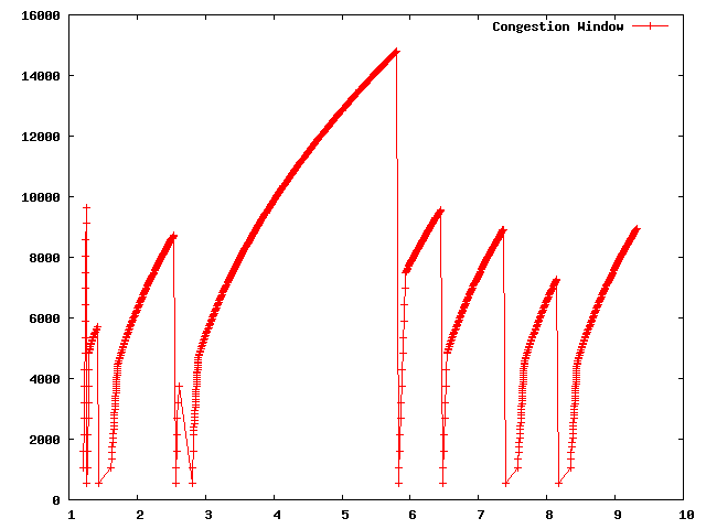
You can now run gnuplot (if you have it installed) and tell it to generate some pretty pictures:
  gnuplot> set terminal png size 640,480
  gnuplot> set output "cwnd.png"
  gnuplot> plot "cwnd.dat" using 1:2 title 'Congestion Window' with linespoints
  gnuplot> exit
You should now have a graph of the congestion window versus time sitting in the file “cwnd.png” in all of its glory, that looks like:
| [ < ] | [ > ] | [ << ] | [ Up ] | [ >> ] | [Top] | [Contents] | [Index] | [ ? ] |
In the previous section, we showed how to hook a trace source and get hopefully
interesting information out of a simulation. Perhaps you will recall that we
called logging to the standard output using std::cout a “Blunt Instrument”
much earlier in this chapter. We also wrote about how it was a problem having
to parse the log output in order to isolate interesting information. It may
have occurred to you that we just spent a lot of time implementing an example
that exhibits all of the problems we purport to fix with the ns-3 tracing
system! You would be correct. But, bear with us. We’re not done yet.
One of the most important things we want to do is to is to have the ability to
easily control the amount of output coming out of the simulation; and we also
want to save those data to a file so we can refer back to it later. We can use
the mid-level trace helpers provided in ns-3 to do just that and complete
the picture.
We provide a script that writes the cwnd change and drop events developed in
the example fifth.cc to disk in separate files. The cwnd changes are
stored as a tab-separated ASCII file and the drop events are stored in a pcap
file. The changes to make this happen are quite small.
| [ < ] | [ > ] | [ << ] | [ Up ] | [ >> ] | [Top] | [Contents] | [Index] | [ ? ] |
Let’s take a look at the changes required to go from fifth.cc to
sixth.cc. Open examples/tutorial/fifth.cc in your favorite
editor. You can see the first change by searching for CwndChange. You will
find that we have changed the signatures for the trace sinks and have added
a single line to each sink that writes the traced information to a stream
representing a file.
  static void
  CwndChange (Ptr<OutputStreamWrapper> stream, uint32_t oldCwnd, uint32_t newCwnd)
  {
    NS_LOG_UNCOND (Simulator::Now ().GetSeconds () << "\t" << newCwnd);
    *stream->GetStream () << Simulator::Now ().GetSeconds () << "\t" << oldCwnd << "\t" << newCwnd << std::endl;
  }

  static void
  RxDrop (Ptr<PcapFileWrapper> file, Ptr<const Packet> p)
  {
    NS_LOG_UNCOND ("RxDrop at " << Simulator::Now ().GetSeconds ());
    file->Write(Simulator::Now(), p);
  }
We have added a “stream” parameter to the CwndChange trace sink.
This is an object that holds (keeps safely alive) a C++ output stream. It
turns out that this is a very simple object, but one that manages lifetime
issues for the stream and solves a problem that even experienced C++ users
run into. It turns out that the copy constructor for ostream is marked
private. This means that ostreams do not obey value semantics and cannot
be used in any mechanism that requires the stream to be copied. This includes
the ns-3 callback system, which as you may recall, requires objects
that obey value semantics. Further notice that we have added the following
line in the CwndChange trace sink implementation:
*stream->GetStream () << Simulator::Now ().GetSeconds () << "\t" << oldCwnd << "\t" << newCwnd << std::endl;
This would be very familiar code if you replaced *stream->GetStream ()
with std::cout, as in:
std::cout << Simulator::Now ().GetSeconds () << "\t" << oldCwnd << "\t" << newCwnd << std::endl;
This illustrates that the Ptr<OutputStreamWrapper> is really just
carrying around a std::ofstream for you, and you can use it here like
any other output stream.
A similar situation happens in RxDrop except that the object being
passed around (a Ptr<PcapFileWrapper>) represents a pcap file. There
is a one-liner in the trace sink to write a timestamp and the contents of the
packet being dropped to the pcap file:
file->Write(Simulator::Now(), p);
Of course, if we have objects representing the two files, we need to create
them somewhere and also cause them to be passed to the trace sinks. If you
look in the main function, you will find new code to do just that:
  AsciiTraceHelper asciiTraceHelper;
  Ptr<OutputStreamWrapper> stream = asciiTraceHelper.CreateFileStream ("sixth.cwnd");
  ns3TcpSocket->TraceConnectWithoutContext ("CongestionWindow", MakeBoundCallback (&CwndChange, stream));

  ...

  PcapHelper pcapHelper;
  Ptr<PcapFileWrapper> file = pcapHelper.CreateFile ("sixth.pcap", std::ios::out, PcapHelper::DLT_PPP);
  devices.Get (1)->TraceConnectWithoutContext("PhyRxDrop", MakeBoundCallback (&RxDrop, file));
In the first section of the code snippet above, we are creating the ASCII trace file, creating an object responsible for managing it and using a variant of the callback creation function to arrange for the object to be passed to the sink. Our ASCII trace helpers provide a rich set of functions to make using text (ASCII) files easy. We are just going to illustrate the use of the file stream creation function here.
The CreateFileStream{ function is basically going to instantiate
a std::ofstream object and create a new file (or truncate an existing file).
This ofstream is packaged up in an ns-3 object for lifetime management
and copy constructor issue resolution.
We then take this ns-3 object representing the file and pass it to
MakeBoundCallback(). This function creates a callback just like
MakeCallback(), but it “binds” a new value to the callback. This
value is added to the callback before it is called.
Essentially, MakeBoundCallback(&CwndChange, stream) causes the trace
source to add the additional “stream” parameter to the front of the formal
parameter list before invoking the callback. This changes the required
signature of the CwndChange sink to match the one shown above, which
includes the “extra” parameter Ptr<OutputStreamWrapper> stream.
In the second section of code in the snippet above, we instantiate a
PcapHelper to do the same thing for our pcap trace file that we did
with the AsciiTraceHelper. The line of code,
Ptr<PcapFileWrapper> file = pcapHelper.CreateFile ("sixth.pcap", "w", PcapHelper::DLT_PPP);
creates a pcap file named “sixth.pcap” with file mode “w”. This means that
the new file is to truncated if an existing file with that name is found. The
final parameter is the “data link type” of the new pcap file. These are
the same as the pcap library data link types defined in bpf.h if you are
familar with pcap. In this case, DLT_PPP indicates that the pcap file
is going to contain packets prefixed with point to point headers. This is true
since the packets are coming from our point-to-point device driver. Other
common data link types are DLT_EN10MB (10 MB Ethernet) appropriate for csma
devices and DLT_IEEE802_11 (IEEE 802.11) appropriate for wifi devices. These
are defined in src/helper/trace-helper.h" if you are interested in seeing
the list. The entries in the list match those in bpf.h but we duplicate
them to avoid a pcap source dependence.
A ns-3 object representing the pcap file is returned from CreateFile
and used in a bound callback exactly as it was in the ascii case.
An important detour: It is important to notice that even though both of these objects are declared in very similar ways,
  Ptr<PcapFileWrapper> file ...
  Ptr<OutputStreamWrapper> stream ...
The underlying objects are entirely different. For example, the
Ptr<PcapFileWrapper> is a smart pointer to an ns-3 Object that is a
fairly heaviweight thing that supports Attributes and is integrated into
the config system. The Ptr<OutputStreamWrapper>, on the other hand, is a smart
pointer to a reference counted object that is a very lightweight thing.
Remember to always look at the object you are referencing before making any
assumptions about the “powers” that object may have.
For example, take a look at src/common/pcap-file-object.h in the
distribution and notice,
class PcapFileWrapper : public Object
that class PcapFileWrapper is an ns-3 Object by virtue of
its inheritance. Then look at src/common/output-stream-wrapper.h and
notice,
class OutputStreamWrapper : public SimpleRefCount<OutputStreamWrapper>
that this object is not an ns-3 Object at all, it is “merely” a
C++ object that happens to support intrusive reference counting.
The point here is that just because you read Ptr<something> it does not necessarily
mean that “something” is an ns-3 Object on which you can hang ns-3
Attributes, for example.
Now, back to the example. If you now build and run this example,
./waf --run sixth
you will see the same messages appear as when you ran “fifth”, but two new
files will appear in the top-level directory of your ns-3 distribution.
sixth.cwnd sixth.pcap
Since “sixth.cwnd” is an ASCII text file, you can view it with cat
or your favorite file viewer.
  1.20919 536     1072
  1.21511 1072    1608
  ...
  9.30922 8893    8925
  9.31754 8925    8957
You have a tab separated file with a timestamp, an old congestion window and a new congestion window suitable for directly importing into your plot program. There are no extraneous prints in the file, no parsing or editing is required.
Since “sixth.pcap” is a pcap file, you can fiew it with tcpdump.
  reading from file ../../sixth.pcap, link-type PPP (PPP)
  1.251507 IP 10.1.1.1.49153 > 10.1.1.2.8080: . 17689:18225(536) ack 1 win 65535
  1.411478 IP 10.1.1.1.49153 > 10.1.1.2.8080: . 33808:34312(504) ack 1 win 65535
  ...
  7.393557 IP 10.1.1.1.49153 > 10.1.1.2.8080: . 781568:782072(504) ack 1 win 65535
  8.141483 IP 10.1.1.1.49153 > 10.1.1.2.8080: . 874632:875168(536) ack 1 win 65535
You have a pcap file with the packets that were dropped in the simulation. There are no other packets present in the file and there is nothing else present to make life difficult.
It’s been a long journey, but we are now at a point where we can appreciate the
ns-3 tracing system. We have pulled important events out of the middle
of a TCP implementation and a device driver. We stored those events directly in
files usable with commonly known tools. We did this without modifying any of the
core code involved, and we did this in only 18 lines of code:
  static void
  CwndChange (Ptr<OutputStreamWrapper> stream, uint32_t oldCwnd, uint32_t newCwnd)
  {
    NS_LOG_UNCOND (Simulator::Now ().GetSeconds () << "\t" << newCwnd);
    *stream->GetStream () << Simulator::Now ().GetSeconds () << "\t" << oldCwnd << "\t" << newCwnd << std::endl;
  }

  ...

  AsciiTraceHelper asciiTraceHelper;
  Ptr<OutputStreamWrapper> stream = asciiTraceHelper.CreateFileStream ("sixth.cwnd");
  ns3TcpSocket->TraceConnectWithoutContext ("CongestionWindow", MakeBoundCallback (&CwndChange, stream));

  ...

  static void
  RxDrop (Ptr<PcapFileWrapper> file, Ptr<const Packet> p)
  {
    NS_LOG_UNCOND ("RxDrop at " << Simulator::Now ().GetSeconds ());
    file->Write(Simulator::Now(), p);
  }

  ...

  PcapHelper pcapHelper;
  Ptr<PcapFileWrapper> file = pcapHelper.CreateFile ("sixth.pcap", "w", PcapHelper::DLT_PPP);
  devices.Get (1)->TraceConnectWithoutContext("PhyRxDrop", MakeBoundCallback (&RxDrop, file));
| [ < ] | [ > ] | [ << ] | [ Up ] | [ >> ] |
This document was generated by root on May 3, 2010 using texi2html 1.82.