
ns-3 Manual
This is the ns-3 Manual. Primary documentation for the ns-3 project is organized as follows:
Several guides that are version controlled for each release (the latest release) and development tree:
Tutorial
Installation Guide
Manual (this document)
Model Library
Contributing Guide
ns-3 Doxygen: Documentation of the public APIs of the simulator
This document is written in reStructuredText for Sphinx and is maintained in the
doc/manual directory of ns-3’s source code. Source file column width is 100 columns.
1. Organization
This chapter describes the overall ns-3 software organization and the corresponding organization of this manual.
ns-3 is a discrete-event network simulator in which the simulation core and models are implemented in C++. ns-3 is built as a library which may be statically or dynamically linked to a C++ main program that defines the simulation topology and starts the simulator. ns-3 also exports nearly all of its API to Python, allowing Python programs to import an “ns3” module in much the same way as the ns-3 library is linked by executables in C++.
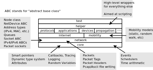
Software organization of ns-3
The source code for ns-3 is mostly organized in the src directory and
can be described by the diagram in Software organization of ns-3. We will
work our way from the bottom up; in general, modules only have dependencies
on modules beneath them in the figure.
We first describe the core of the simulator; those components that are
common across all protocol, hardware, and environmental models.
The simulation core is implemented in src/core. Packets are
fundamental objects in a network simulator
and are implemented in src/network. These two simulation modules by
themselves are intended to comprise a generic simulation core that can be
used by different kinds of networks, not just Internet-based networks. The
above modules of ns-3 are independent of specific network and device
models, which are covered in subsequent parts of this manual.
In addition to the above ns-3 core, we introduce, also in the initial portion of the manual, two other modules that supplement the core C++-based API. ns-3 programs may access all of the API directly or may make use of a so-called helper API that provides convenient wrappers or encapsulation of low-level API calls. The fact that ns-3 programs can be written to two APIs (or a combination thereof) is a fundamental aspect of the simulator. We also describe how Python is supported in ns-3 before moving onto specific models of relevance to network simulation.
The remainder of the manual is focused on documenting the models and
supporting capabilities. The next part focuses on two fundamental objects in
ns-3: the Node and NetDevice. Two special NetDevice types are
designed to support network emulation use cases, and emulation is described
next. The following chapter is devoted to Internet-related models,
including the
sockets API used by Internet applications. The next chapter covers
applications, and the following chapter describes additional support for
simulation, such as animators and statistics.
The project maintains a manual section devoted to testing and validation of ns-3 code (see the tests section in the ns-3 manual).
2. Simulator
This chapter explains some of the core ns-3 simulator concepts.
2.1. Events and Simulator
ns-3 is a discrete-event network simulator. Conceptually, the simulator keeps track of a number of events that are scheduled to execute at a specified simulation time. The job of the simulator is to execute the events in sequential time order. Once the completion of an event occurs, the simulator will move to the next event (or will exit if there are no more events in the event queue). If, for example, an event scheduled for simulation time “100 seconds” is executed, and the next event is not scheduled until “200 seconds”, the simulator will immediately jump from 100 seconds to 200 seconds (of simulation time) to execute the next event. This is what is meant by “discrete-event” simulator.
To make this all happen, the simulator needs a few things:
a simulator object that can access an event queue where events are stored and that can manage the execution of events
a scheduler responsible for inserting and removing events from the queue
a way to represent simulation time
the events themselves
This chapter of the manual describes these fundamental objects (simulator, scheduler, time, event) and how they are used.
2.1.1. Event
An event represents something that changes the simulation status, i.e., between two events the simulation status does not change, and the event will likely change it (it could also not change anything).
Note that another way to understand an event is to consider it as a delayed function call. With the due differences, a discrete event simulation is not much different from a “normal” program where the functions are not called immediately, but are marked with a “time”, and the time is used to decide the order of the functions execution.
The time, of course, is a simulated time, and is quite different from the “real” time. Depending on the simulation complexity the simulated time can advance faster or slower then the “real” time, but like a “real” time can only go forward.
An example of an event is the reception of a packet, or the expiration of a timer.
An event is represented by:
The time at which the event will happen
A pointer to the function that will “handle” the event,
The parameters of the function that will handle the event (if any),
Other internal structures.
An event is scheduled through a call to Simulator::Schedule, and once
scheduled, it can be canceled or removed.
Removal implies removal from the scheduler data structure, while cancel
keeps them in the data structure but sets a boolean flag that suppresses
calling the bound event function at the scheduled time. When an event is
scheduled by the Simulator, an EventId is returned. The client may use
this event ID to later cancel or remove the event; see the example program
src/core/examples/sample-simulator.{cc,py} for example usage.
Cancelling an event is typically less computationally expensive than
removing it, but cancelled events consumes more memory in the scheduler
data structure, which might impact its performances.
Events are stored by the simulator in a scheduler data structure. Events are handled in increasing order of simulator time, and in the case of two events with the same scheduled time, the event with the lowest unique ID (a monotonically increasing counter) will be handled first. In other words tied events are handled in FIFO order.
Note that concurrent events (events that happen at the very same time) are unlikely in a real system - not to say impossible. In ns-3 concurrent events are common for a number of reasons, one of them being the time representation. While developing a model this must be carefully taken into account.
During the event execution, the simulation time will not advance, i.e., each event is executed in zero time. This is a common assumption in discrete event simulations, and holds when the computational complexity of the operations executed in the event is negligible. When this assumption does not hold, it is necessary to schedule a second event to mimic the end of the computationally intensive task.
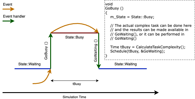
As an example, suppose to have a device that receives a packet and has to perform a complex analysis on it (e.g., an image processing task). The sequence of events will be:
T(t) - Packet reception and processing, save the result somewhere, and schedule an event in (t+d) marking the end of the data processing.
T(t+d) - Retrieve the data, and do other stuff based them.
So, even if the data processing actually did return a result in the execution of the first event, the data is considered valid only after the second event.
The image below can be useful to clarify the idea.
2.1.2. Simulator
The Simulator class is the public entry point to access event scheduling
facilities. Once a couple of events have been scheduled to start the
simulation, the user can start to execute them by entering the simulator
main loop (call Simulator::Run). Once the main loop starts running, it
will sequentially execute all scheduled events in order from oldest to
most recent until there are either no more events left in the event
queue or Simulator::Stop has been called.
To schedule events for execution by the simulator main loop, the Simulator class provides the Simulator::Schedule* family of functions.
Handling event handlers with different signatures
These functions are declared and implemented as C++ templates to handle automatically the wide variety of C++ event handler signatures used in the wild. For example, to schedule an event to execute 10 seconds in the future, and invoke a C++ method or function with specific arguments, you might write this:
void handler(int arg0, int arg1)
{
  std::cout << "handler called with argument arg0=" << arg0 << " and
     arg1=" << arg1 << std::endl;
}

Simulator::Schedule(Seconds(10), &handler, 10, 5);
Which will output:
handler called with argument arg0=10 and arg1=5
Of course, these C++ templates can also handle transparently member methods on C++ objects:
To be completed: member method example
Notes:
the ns-3 Schedule methods recognize automatically functions and methods only if they take less than 5 arguments. If you need them to support more arguments, please, file a bug report.
Readers familiar with the term ‘fully-bound functors’ will recognize the Simulator::Schedule methods as a way to automatically construct such objects.
Common scheduling operations
The Simulator API was designed to make it really simple to schedule most events. It provides three variants to do so (ordered from most commonly used to least commonly used):
Schedulemethods which allow you to schedule an event in the future by providing the delay between the current simulation time and the expiration date of the target event.ScheduleNowmethods which allow you to schedule an event for the current simulation time: they will execute _after_ the current event is finished executing but _before_ the simulation time is changed for the next event.ScheduleDestroymethods which allow you to hook in the shutdown process of the Simulator to cleanup simulation resources: every ‘destroy’ event is executed when the user calls the Simulator::Destroy method.
Maintaining the simulation context
There are two basic ways to schedule events, with and without context. What does this mean?
Simulator::Schedule(Time const &time, MEM mem_ptr, OBJ obj);
vs.
Simulator::ScheduleWithContext(uint32_t context, Time const &time, MEM mem_ptr, OBJ obj);
Readers who invest time and effort in developing or using a non-trivial simulation model will know the value of the ns-3 logging framework to debug simple and complex simulations alike. One of the important features that is provided by this logging framework is the automatic display of the network node id associated with the ‘currently’ running event.
The node id of the currently executing network node is in fact tracked by the Simulator class. It can be accessed with the Simulator::GetContext method which returns the ‘context’ (a 32-bit integer) associated and stored in the currently-executing event. In some rare cases, when an event is not associated with a specific network node, its ‘context’ is set to 0xffffffff.
To associate a context to each event, the Schedule, and ScheduleNow methods automatically reuse the context of the currently-executing event as the context of the event scheduled for execution later.
In some cases, most notably when simulating the transmission of a packet from a node to another, this behavior is undesirable since the expected context of the reception event is that of the receiving node, not the sending node. To avoid this problem, the Simulator class provides a specific schedule method: ScheduleWithContext which allows one to provide explicitly the node id of the receiving node associated with the receive event.
XXX: code example
In some very rare cases, developers might need to modify or understand how the context (node id) of the first event is set to that of its associated node. This is accomplished by the NodeList class: whenever a new node is created, the NodeList class uses ScheduleWithContext to schedule a ‘initialize’ event for this node. The ‘initialize’ event thus executes with a context set to that of the node id and can use the normal variety of Schedule methods. It invokes the Node::Initialize method which propagates the ‘initialize’ event by calling the DoInitialize method for each object associated with the node. The DoInitialize method overridden in some of these objects (most notably in the Application base class) will schedule some events (most notably Application::StartApplication) which will in turn scheduling traffic generation events which will in turn schedule network-level events.
Notes:
Users need to be careful to propagate DoInitialize methods across objects by calling Initialize explicitly on their member objects
The context id associated with each ScheduleWithContext method has other uses beyond logging: it is used by an experimental branch of ns-3 to perform parallel simulation on multicore systems using multithreading.
The Simulator::* functions do not know what the context is: they merely make sure that whatever context you specify with ScheduleWithContext is available when the corresponding event executes with ::GetContext.
It is up to the models implemented on top of Simulator::* to interpret the context value. In ns-3, the network models interpret the context as the node id of the node which generated an event. This is why it is important to call ScheduleWithContext in ns3::Channel subclasses because we are generating an event from node i to node j and we want to make sure that the event which will run on node j has the right context.
2.1.2.1. Available Simulator Engines
ns-3 supplies two different types of basic simulator engine to manage event execution. These are derived from the abstract base class SimulatorImpl:
DefaultSimulatorImpl This is a classic sequential discrete event simulator engine which uses a single thread of execution. This engine executes events as fast as possible.
DistributedSimulatorImpl This is a classic YAWNS distributed (“parallel”) simulator engine. By labeling and instantiating your model components appropriately this engine will execute the model in parallel across many compute processes, yet in a time-synchronized way, as if the model had executed sequentially. The two advantages are to execute models faster and to execute models too large to fit in one compute node. This engine also attempts to execute as fast as possible.
NullMessageSimulatorImpl This implements a variant of the Chandy- Misra-Bryant (CMB) null message algorithm for parallel simulation. Like DistributedSimulatorImpl this requires appropriate labeling and instantiation of model components. This engine attempts to execute events as fast as possible.
You can choose which simulator engine to use by setting a global variable, for example:
GlobalValue::Bind("SimulatorImplementationType",
                  StringValue("ns3::DistributedSimulatorImpl"));
or by using a command line argument
$ ./ns3 run "... --SimulatorImplementationType=ns3::DistributedSimulatorImpl"
In addition to the basic simulator engines there is a general facility used to build “adapters” which provide small behavior modifications to one of the core SimulatorImpl engines. The adapter base class is SimulatorAdapter, itself derived from SimulatorImpl. SimulatorAdapter uses the PIMPL (pointer to implementation) idiom to forward all calls to the configured base simulator engine. This makes it easy to provide small customizations just by overriding the specific Simulator calls needed, and allowing SimulatorAdapter to handle the rest.
There are few places where adapters are used currently:
RealtimeSimulatorImpl This adapter attempts to execute in real time by pacing the wall clock evolution. This pacing is “best effort”, meaning actual event execution may not occur exactly in sync, but close to it. This engine is normally only used with the DefaultSimulatorImpl, but it can be used to keep a distributed simulation synchronized with real time. See the RealTime chapter.
VisualSimulatorImpl This adapter starts a live visualization of the running simulation, showing the network graph and each packet traversing the links.
LocalTimeSimulatorImpl This adapter enables attaching noisy local clocks to Nodes, then scheduling events with respect to the local noisy clock, instead of relative to the true simulator time.
In addition to the PIMPL idiom of SimulatorAdapter there is a special per-event customization hook:
SimulatorImpl::PreEventHook( const EventId & id)
One can use this to perform any housekeeping actions before the next event actually executes.
The distinction between a core engine and an adapter is the following: there can only ever be one core engine running, while there can be several adapters chained up each providing a variation on the base engine execution. For example one can use noisy local clocks with the real time adapter.
A single adapter can be added on top of the DefaultSimulatorImpl by the same two methods above: binding the “SimulatorImplementationType” global value or using the command line argument. To chain multiple adapters a different approach must be used; see the SimulatorAdapter::AddAdapter() API documentation.
The simulator engine type can be set once, but must be set before the first call to the Simulator() API. In practice, since some models have to schedule their start up events when they are constructed, this means generally you should set the engine type before instantiating any other model components.
The engine type can be changed after Simulator::Destroy() but before any additional calls to the Simulator API, for instance when executing multiple runs in a single ns-3 invocation.
2.1.3. Time
ns-3 internally represents simulation times and durations as 64-bit signed integers (with the sign bit used for negative durations). The time values are interpreted with respect to a “resolution” unit in the customary SI units: fs, ps, ns, us, ms, s, min, h, d, y. The unit defines the minimum Time value. It can be changed once before any calls to Simulator::Run(). It is not stored with the 64-bit time value itself.
Times can be constructed from all standard numeric types (using the configured default unit) or with explicit units (as in Time MicroSeconds (uint64_t value)). Times can be compared, tested for sign or equality to zero, rounded to a given unit, converted to standard numeric types in specific units. All basic arithmetic operations are supported (addition, subtraction, multiplication or division by a scalar (numeric value)). Times can be written to/read from IO streams. In the case of writing it is easy to choose the output unit, different from the resolution unit.
Here are examples of common usage:
Time t1 = MilliSeconds(1500); // 1.5 s = 1500 ms
Time t2 = MicroSeconds(500);  // 500 microseconds
Time t3 = t1 + t2;            // arithmetic
Time t4 = t3 * 2;             // multiplication

if (t4 > Seconds(3))
{
    std::cout << "t4 is greater than 3 seconds\n";
}

double ms = t4.GetMilliSeconds(); // convert to double in ms

std::cout << t4.As(Time::MS) << "\n"; // stream with specific unit
Note
When using floating-point values with constructors like Seconds(1.5),
users should be aware that values smaller than the current resolution
will be rounded. For example, if the resolution is set to nanoseconds,
values like Seconds(1e-10) will be rounded to zero.
Consider inspecting Time::SetResolution() and using methods like
GetNanoSeconds() to understand how sub-resolution values behave in practice.
When calling Time::SetResolution(), there is a trade-off between
the precision of time measurements and the maximum simulation time
span that can be represented. Finer resolutions (like femtoseconds)
allow for more precise timing but reduce the maximum representable
duration.
Resolution Unit |
Smallest Step |
Approximate Max Time Span |
|---|---|---|
Seconds |
1 s |
~2.9 × 10¹¹ years |
Milliseconds |
1 ms |
~2.9 × 10⁸ years |
Microseconds |
1 µs |
~2.9 × 10⁵ years |
Nanoseconds |
1 ns |
~292 years |
Picoseconds |
1 ps |
~107 days |
Femtoseconds |
1 fs |
~2.6 hours |
2.1.4. Scheduler
The main job of the Scheduler classes is to maintain the priority queue of future events. The scheduler can be set with a global variable, similar to choosing the SimulatorImpl:
GlobalValue::Bind("SchedulerType",
                  StringValue("ns3::DistributedSimulatorImpl"));
The scheduler can be changed at any time via Simulator::SetScheduler(). The default scheduler is MapScheduler which uses a std::map<> to store events in time order.
Because event distributions vary by model there is no one best strategy for the priority queue, so ns-3 has several options with differing tradeoffs. The example utils/bench-scheduler.c can be used to test the performance for a user-supplied event distribution. For modest execution times (less than an hour, say) the choice of priority queue is usually not significant; configuring the build type to optimized is much more important in reducing execution times.
The available scheduler types, and a summary of their time and space complexity on Insert() and RemoveNext(), are listed in the following table. See the individual Scheduler API pages for details on the complexity of the other API calls.
Scheduler Type |
Complexity |
||||
|---|---|---|---|---|---|
SchedulerImpl Type |
Method |
Time |
Space |
||
Insert() |
RemoveNext() |
Overhead |
Per Event |
||
CalendarScheduler |
<std::list> [] |
Constant |
Constant |
24 bytes |
16 bytes |
HeapScheduler |
Heap on std::vector |
Logarithmic |
Logarithmic |
24 bytes |
0 |
ListScheduler |
std::list |
Linear |
Constant |
24 bytes |
16 bytes |
MapScheduler |
st::map |
Logarithmic |
Constant |
40 bytes |
32 bytes |
PriorityQueueScheduler |
std::priority_queue<,std::vector> |
Logarithmic |
Logarithms |
24 bytes |
0 |
2.2. Callbacks
Some new users to ns-3 are unfamiliar with an extensively used programming idiom used throughout the code: the ns-3 callback. This chapter provides some motivation on the callback, guidance on how to use it, and details on its implementation.
2.2.1. Callbacks Motivation
Consider that you have two simulation models A and B, and you wish to have them pass information between them during the simulation. One way that you can do that is that you can make A and B each explicitly knowledgeable about the other, so that they can invoke methods on each other:
class A {
public:
  void ReceiveInput( /* parameters */ );
  ...
}
and in another source file:
class B {
public:
  void DoSomething();
  ...

private:
  A* a_instance; // pointer to an A
}

void
B::DoSomething()
{
  // Tell a_instance that something happened
  a_instance->ReceiveInput( /* parameters */ );
  ...
}
This certainly works, but it has the drawback that it introduces a dependency on
A and B to know about the other at compile time (this makes it harder to have
independent compilation units in the simulator) and is not generalized; if in a
later usage scenario, B needs to talk to a completely different C object, the
source code for B needs to be changed to add a c_instance and so forth. It
is easy to see that this is a brute force mechanism of communication that can
lead to programming cruft in the models.
This is not to say that objects should not know about one another if there is a hard dependency between them, but that often the model can be made more flexible if its interactions are less constrained at compile time.
This is not an abstract problem for network simulation research, but rather it has been a source of problems in previous simulators, when researchers want to extend or modify the system to do different things (as they are apt to do in research). Consider, for example, a user who wants to add an IPsec security protocol sublayer between TCP and IP:
If the simulator has made assumptions, and hard coded into the code, that IP always talks to a transport protocol above, the user may be forced to hack the system to get the desired interconnections. This is clearly not an optimal way to design a generic simulator.
2.2.2. Callbacks Background
Note
Readers familiar with programming callbacks may skip this tutorial section.
The basic mechanism that allows one to address the problem above is known as a callback. The ultimate goal is to allow one piece of code to call a function (or method in C++) without any specific inter-module dependency.
This ultimately means you need some kind of indirection – you treat the address of the called function as a variable. This variable is called a pointer-to-function variable. The relationship between function and pointer-to-function pointer is really no different that that of object and pointer-to-object.
In C the canonical example of a pointer-to-function is a pointer-to-function-returning-integer (PFI). For a PFI taking one int parameter, this could be declared like,:
int (*pfi)(int arg) = 0;
What you get from this is a variable named simply pfi that is initialized to
the value 0. If you want to initialize this pointer to something meaningful, you
have to have a function with a matching signature. In this case:
int MyFunction(int arg) {}
If you have this target, you can initialize the variable to point to your function like:
pfi = MyFunction;
You can then call MyFunction indirectly using the more suggestive form of the call:
int result = (*pfi)(1234);
This is suggestive since it looks like you are dereferencing the function pointer just like you would dereference any pointer. Typically, however, people take advantage of the fact that the compiler knows what is going on and will just use a shorter form:
int result = pfi(1234);
Notice that the function pointer obeys value semantics, so you can pass it around like any other value. Typically, when you use an asynchronous interface you will pass some entity like this to a function which will perform an action and call back to let you know it completed. It calls back by following the indirection and executing the provided function.
In C++ you have the added complexity of objects. The analogy with the PFI above means you have a pointer to a member function returning an int (PMI) instead of the pointer to function returning an int (PFI).
The declaration of the variable providing the indirection looks only slightly different:
int (MyClass::*pmi)(int arg) = 0;
This declares a variable named pmi just as the previous example declared a
variable named pfi. Since the will be to call a method of an instance of a
particular class, one must declare that method in a class:
class MyClass {
public:
  int MyMethod(int arg);
};
Given this class declaration, one would then initialize that variable like this:
pmi = &MyClass::MyMethod;
This assigns the address of the code implementing the method to the variable,
completing the indirection. In order to call a method, the code needs a this
pointer. This, in turn, means there must be an object of MyClass to refer to. A
simplistic example of this is just calling a method indirectly (think virtual
function):
int (MyClass::*pmi)(int arg) = 0;   // Declare a PMI
pmi = &MyClass::MyMethod;           // Point at the implementation code

MyClass myClass;                    // Need an instance of the class
(myClass.*pmi)(1234);              // Call the method with an object ptr
Just like in the C example, you can use this in an asynchronous call to another module which will call back using a method and an object pointer. The straightforward extension one might consider is to pass a pointer to the object and the PMI variable. The module would just do:
(*objectPtr.*pmi)(1234);
to execute the callback on the desired object.
One might ask at this time, what’s the point? The called module will have to
understand the concrete type of the calling object in order to properly make the
callback. Why not just accept this, pass the correctly typed object pointer and
do object->Method(1234) in the code instead of the callback? This is
precisely the problem described above. What is needed is a way to decouple the
calling function from the called class completely. This requirement led to the
development of the Functor.
A functor is the outgrowth of something invented in the 1960s called a closure. It is basically just a packaged-up function call, possibly with some state.
A functor has two parts, a specific part and a generic part, related through
inheritance. The calling code (the code that executes the callback) will execute
a generic overloaded operator() of a generic functor to cause the callback
to be called. The called code (the code that wants to be called back) will have
to provide a specialized implementation of the operator() that performs the
class-specific work that caused the close-coupling problem above.
With the specific functor and its overloaded operator() created, the called
code then gives the specialized code to the module that will execute the
callback (the calling code).
The calling code will take a generic functor as a parameter, so an implicit cast is done in the function call to convert the specific functor to a generic functor. This means that the calling module just needs to understand the generic functor type. It is decoupled from the calling code completely.
The information one needs to make a specific functor is the object pointer and the pointer-to-method address.
The essence of what needs to happen is that the system declares a generic part of the functor:
template <typename T>
class Functor
{
public:
  virtual int operator()(T arg) = 0;
};
The caller defines a specific part of the functor that really is just there to
implement the specific operator() method:
template <typename T, typename ARG>
class SpecificFunctor : public Functor<ARG>
{
public:
  SpecificFunctor(T* p, int (T::*_pmi)(ARG arg))
  {
    m_p = p;
    m_pmi = _pmi;
  }

  virtual int operator()(ARG arg)
  {
    (*m_p.*m_pmi)(arg);
  }
private:
  int (T::*m_pmi)(ARG arg);
  T* m_p;
};
Here is an example of the usage:
class A
{
public:
A(int a0) : a(a0) {}
int Hello(int b0)
{
  std::cout << "Hello from A, a = " << a << " b0 = " << b0 << std::endl;
}
int a;
};

int main()
{
  A a(10);
  SpecificFunctor<A, int> sf(&a, &A::Hello);
  sf(5);
}
Note
The previous code is not real ns-3 code. It is simplistic example code used only to illustrate the concepts involved and to help you understand the system more. Do not expect to find this code anywhere in the ns-3 tree.
Notice that there are two variables defined in the class above. The m_p variable is the object pointer and m_pmi is the variable containing the address of the function to execute.
Notice that when operator() is called, it in turn calls the method provided
with the object pointer using the C++ PMI syntax.
To use this, one could then declare some model code that takes a generic functor as a parameter:
void LibraryFunction(Functor functor);
The code that will talk to the model would build a specific functor and pass it to LibraryFunction:
MyClass myClass;
SpecificFunctor<MyClass, int> functor(&myclass, MyClass::MyMethod);
When LibraryFunction is done, it executes the callback using the
operator() on the generic functor it was passed, and in this particular
case, provides the integer argument:
void
LibraryFunction(Functor functor)
{
  // Execute the library function
  functor(1234);
}
Notice that LibraryFunction is completely decoupled from the specific
type of the client. The connection is made through the Functor polymorphism.
The Callback API in ns-3 implements object-oriented callbacks using the functor mechanism. This callback API, being based on C++ templates, is type-safe; that is, it performs static type checks to enforce proper signature compatibility between callers and callees. It is therefore more type-safe to use than traditional function pointers, but the syntax may look imposing at first. This section is designed to walk you through the Callback system so that you can be comfortable using it in ns-3.
2.2.3. Using the Callback API
The Callback API is fairly minimal, providing only two services:
1. callback type declaration: a way to declare a type of callback with a given signature, and,
2. callback instantiation: a way to instantiate a template-generated forwarding callback which can forward any calls to another C++ class member method or C++ function.
This is best observed via walking through an example, based on
samples/main-callback.cc.
2.2.3.1. Using the Callback API with static functions
Consider a function:
static double
CbOne(double a, double b)
{
  std::cout << "invoke cbOne a=" << a << ", b=" << b << std::endl;
  return a;
}
Consider also the following main program snippet:
int main(int argc, char *argv[])
{
  // return type: double
  // first arg type: double
  // second arg type: double
  Callback<double, double, double> one;
}
This is an example of a C-style callback – one which does not include or need
a this pointer. The function template Callback is essentially the
declaration of the variable containing the pointer-to-function. In the example
above, we explicitly showed a pointer to a function that returned an integer and
took a single integer as a parameter, The Callback template function is
a generic version of that – it is used to declare the type of a callback.
Note
Readers unfamiliar with C++ templates may consult http://www.cplusplus.com/doc/tutorial/templates/.
The Callback template requires one mandatory argument (the return type
of the function to be assigned to this callback) and up to five optional
arguments, which each specify the type of the arguments (if your particular
callback function has more than five arguments, then this can be handled
by extending the callback implementation).
So in the above example, we have a declared a callback named “one” that will
eventually hold a function pointer. The signature of the function that it will
hold must return double and must support two double arguments. If one tries
to pass a function whose signature does not match the declared callback,
a compilation error will occur. Also, if one tries to assign to a callback
an incompatible one, compilation will succeed but a run-time
NS_FATAL_ERROR will be raised. The sample program
src/core/examples/main-callback.cc demonstrates both of these error cases
at the end of the main() program.
Now, we need to tie together this callback instance and the actual target function (CbOne). Notice above that CbOne has the same function signature types as the callback– this is important. We can pass in any such properly-typed function to this callback. Let’s look at this more closely:
static   double CbOne(double a, double b) {}
           ^             ^         ^
           |             |         |
           |             |         |
Callback<double,       double,   double> one;
You can only bind a function to a callback if they have the matching signature. The first template argument is the return type, and the additional template arguments are the types of the arguments of the function signature.
Now, let’s bind our callback “one” to the function that matches its signature:
// build callback instance which points to cbOne function
one = MakeCallback(&CbOne);
This call to MakeCallback is, in essence, creating one of the specialized
functors mentioned above. The variable declared using the Callback
template function is going to be playing the part of the generic functor. The
assignment one = MakeCallback(&CbOne) is the cast that converts the
specialized functor known to the callee to a generic functor known to the caller.
Then, later in the program, if the callback is needed, it can be used as follows:
NS_ASSERT(!one.IsNull());

// invoke cbOne function through callback instance
double retOne;
retOne = one(10.0, 20.0);
The check for IsNull() ensures that the callback is not null – that there
is a function to call behind this callback. Then, one() executes the
generic operator() which is really overloaded with a specific implementation
of operator() and returns the same result as if CbOne() had been
called directly.
2.2.3.2. Using the Callback API with member functions
Generally, you will not be calling static functions but instead public member functions of an object. In this case, an extra argument is needed to the MakeCallback function, to tell the system on which object the function should be invoked. Consider this example, also from main-callback.cc:
class MyCb {
public:
  int CbTwo(double a) {
      std::cout << "invoke cbTwo a=" << a << std::endl;
      return -5;
  }
};

int main()
{
  ...
  // return type: int
  // first arg type: double
  Callback<int, double> two;
  MyCb cb;
  // build callback instance which points to MyCb::cbTwo
  two = MakeCallback(&MyCb::CbTwo, &cb);
  ...
}
Here, we pass an additional object pointer to the MakeCallback<> function.
Recall from the background section above that Operator() will use the pointer to
member syntax when it executes on an object:
virtual int operator()(ARG arg)
{
  (*m_p.*m_pmi)(arg);
}
And so we needed to provide the two variables (m_p and m_pmi) when
we made the specific functor. The line:
two = MakeCallback(&MyCb::CbTwo, &cb);
does precisely that. In this case, when two() is invoked:
int result = two(1.0);
will result in a call to the CbTwo member function (method) on the object
pointed to by &cb.
2.2.3.3. Building Null Callbacks
It is possible for callbacks to be null; hence it may be wise to
check before using them. There is a special construct for a null
callback, which is preferable to simply passing “0” as an argument;
it is the MakeNullCallback<> construct:
two = MakeNullCallback<int, double>();
NS_ASSERT(two.IsNull());
Invoking a null callback is just like invoking a null function pointer: it will crash at runtime.
2.2.4. Bound Callbacks
A very useful extension to the functor concept is that of a Bound Callback.
Previously it was mentioned that closures were originally function calls
packaged up for later execution. Notice that in all of the Callback
descriptions above, there is no way to package up any parameters for use
later – when the Callback is called via operator(). All of
the parameters are provided by the calling function.
What if it is desired to allow the client function (the one that provides the
callback) to provide some of the parameters?
Alexandrescu
calls the process of allowing a client to specify one of the parameters “binding”.
One of the parameters of operator() has been bound (fixed) by the client.
Some of our pcap tracing code provides a nice example of this. There is a function that needs to be called whenever a packet is received. This function calls an object that actually writes the packet to disk in the pcap file format. The signature of one of these functions will be:
static void DefaultSink(Ptr<PcapFileWrapper> file, Ptr<const Packet> p);
The static keyword means this is a static function which does not need a
this pointer, so it will be using C-style callbacks. We don’t want the
calling code to have to know about anything but the Packet. What we want in
the calling code is just a call that looks like:
m_promiscSnifferTrace(m_currentPkt);
What we want to do is to bind the Ptr<PcapFileWriter> file to the
specific callback implementation when it is created and arrange for the
operator() of the Callback to provide that parameter for free.
We provide the MakeBoundCallback template function for that purpose. It
takes the same parameters as the MakeCallback template function but also
takes the parameters to be bound. In the case of the example above:
MakeBoundCallback(&DefaultSink, file);
will create a specific callback implementation that knows to add in the extra bound arguments. Conceptually, it extends the specific functor described above with one or more bound arguments:
template <typename T, typename ARG, typename BOUND_ARG>
class SpecificFunctor : public Functor
{
  public:
    SpecificFunctor(T* p, int (T::*_pmi)(ARG arg), BOUND_ARG boundArg)
    {
      m_p = p;
      m_pmi = pmi;
      m_boundArg = boundArg;
    }

    virtual int operator()(ARG arg)
    {
      (*m_p.*m_pmi)(m_boundArg, arg);
    }
  private:
    void (T::*m_pmi)(ARG arg);
    T* m_p;
    BOUND_ARG m_boundArg;
};
You can see that when the specific functor is created, the bound argument is saved
in the functor / callback object itself. When the operator() is invoked with
the single parameter, as in:
m_promiscSnifferTrace(m_currentPkt);
the implementation of operator() adds the bound parameter into the actual
function call:
(*m_p.*m_pmi)(m_boundArg, arg);
It’s possible to bind two or three arguments as well. Say we have a function with signature:
static void NotifyEvent(Ptr<A> a, Ptr<B> b, MyEventType e);
One can create bound callback binding first two arguments like:
MakeBoundCallback(&NotifyEvent, a1, b1);
assuming a1 and b1 are objects of type A and B respectively. Similarly for three arguments one would have function with a signature:
static void NotifyEvent(Ptr<A> a, Ptr<B> b, MyEventType e);
Binding three arguments in done with:
MakeBoundCallback(&NotifyEvent, a1, b1, c1);
again assuming a1, b1 and c1 are objects of type A, B and C respectively.
This kind of binding can be used for exchanging information between objects in simulation; specifically, bound callbacks can be used as traced callbacks, which will be described in the next section.
2.2.5. Traced Callbacks
Placeholder subsection
2.2.6. Callback locations in ns-3
Where are callbacks frequently used in ns-3? Here are some of the more visible ones to typical users:
Socket API
Layer-2/Layer-3 API
Tracing subsystem
API between IP and routing subsystems
2.2.7. Implementation details
The code snippets above are simplistic and only designed to illustrate the mechanism itself. The actual Callback code is quite complicated and very template-intense and a deep understanding of the code is not required. If interested, expert users may find the following useful.
The code was originally written based on the techniques described in http://www.codeproject.com/cpp/TTLFunction.asp. It was subsequently rewritten to follow the architecture outlined in Modern C++ Design, Generic Programming and Design Patterns Applied, Alexandrescu, chapter 5, Generalized Functors.
This code uses:
default template parameters to saves users from having to specify empty parameters when the number of parameters is smaller than the maximum supported number
the pimpl idiom: the Callback class is passed around by value and delegates the crux of the work to its pimpl pointer.
two pimpl implementations which derive from CallbackImpl FunctorCallbackImpl can be used with any functor-type while MemPtrCallbackImpl can be used with pointers to member functions.
a reference list implementation to implement the Callback’s value semantics.
This code most notably departs from the Alexandrescu implementation in that it does not use type lists to specify and pass around the types of the callback arguments. Of course, it also does not use copy-destruction semantics and relies on a reference list rather than autoPtr to hold the pointer.
2.3. Object model
ns-3 is fundamentally a C++ object system. Objects can be declared and instantiated as usual, per C++ rules. ns-3 also adds some features to traditional C++ objects, as described below, to provide greater functionality and features. This manual chapter is intended to introduce the reader to the ns-3 object model.
This section describes the C++ class design for ns-3 objects. In brief, several design patterns in use include classic object-oriented design (polymorphic interfaces and implementations), separation of interface and implementation, the non-virtual public interface design pattern, an object aggregation facility, and reference counting for memory management. Those familiar with component models such as COM or Bonobo will recognize elements of the design in the ns-3 object aggregation model, although the ns-3 design is not strictly in accordance with either.
2.3.1. Object-oriented behavior
C++ objects, in general, provide common object-oriented capabilities (abstraction, encapsulation, inheritance, and polymorphism) that are part of classic object-oriented design. ns-3 objects make use of these properties; for instance:
class Address
{
public:
  Address();
  Address(uint8_t type, const uint8_t *buffer, uint8_t len);
  Address(const Address & address);
  Address &operator=(const Address &address);
  ...
private:
  uint8_t m_type;
  uint8_t m_len;
  ...
};
2.3.2. Object base classes
There are three special base classes used in ns-3. Classes that inherit from these base classes can instantiate objects with special properties. These base classes are:
class
Objectclass
ObjectBaseclass
SimpleRefCount
It is not required that ns-3 objects inherit from these class, but
those that do get special properties. Classes deriving from
class Object get the following properties.
the ns-3 type and attribute system (see Configuration and Attributes)
an object aggregation system
a smart-pointer reference counting system (class Ptr)
Classes that derive from class ObjectBase get the first two
properties above, but do not get smart pointers. Classes that derive from class
SimpleRefCount: get only the smart-pointer reference counting
system.
In practice, class Object is the variant of the three above that
the ns-3 developer will most commonly encounter.
2.3.3. Memory management and class Ptr
Memory management in a C++ program is a complex process, and is often done incorrectly or inconsistently. We have settled on a reference counting design described as follows.
All objects using reference counting maintain an internal reference count to
determine when an object can safely delete itself. Each time that a pointer is
obtained to an interface, the object’s reference count is incremented by calling
Ref(). It is the obligation of the user of the pointer to explicitly
Unref() the pointer when done. When the reference count falls to zero, the
object is deleted.
When the client code obtains a pointer from the object itself through object creation, or via GetObject, it does not have to increment the reference count.
When client code obtains a pointer from another source (e.g., copying a pointer) it must call
Ref()to increment the reference count.All users of the object pointer must call
Unref()to release the reference.
The burden for calling Unref() is somewhat relieved by the use of
the reference counting smart pointer class described below.
Users using a low-level API who wish to explicitly allocate non-reference-counted objects on the heap, using operator new, are responsible for deleting such objects.
2.3.3.1. Reference counting smart pointer (Ptr)
Calling Ref() and Unref() all the time would be cumbersome, so ns-3
provides a smart pointer class Ptr similar to
Boost::intrusive_ptr. This smart-pointer class assumes that the
underlying type provides a pair of Ref and Unref methods that are
expected to increment and decrement the internal refcount of the object
instance.
This implementation allows you to manipulate the smart pointer as if it was a normal pointer: you can compare it with zero, compare it against other pointers, assign zero to it, etc.
It is possible to extract the raw pointer from this smart pointer with the
GetPointer() and PeekPointer() methods.
If you want to store a newed object into a smart pointer, we recommend you to use the CreateObject template functions to create the object and store it in a smart pointer to avoid memory leaks. These functions are really small convenience functions and their goal is just to save you a small bit of typing.
2.3.4. CreateObject and Create
Objects in C++ may be statically, dynamically, or automatically created. This holds true for ns-3 also, but some objects in the system have some additional frameworks available. Specifically, reference counted objects are usually allocated using a templated Create or CreateObject method, as follows.
For objects deriving from class Object:
Ptr<WifiNetDevice> device = CreateObject<WifiNetDevice>();
Please do not create such objects using operator new; create them using
CreateObject() instead.
For objects deriving from class SimpleRefCount, or other objects
that support usage of the smart pointer class, a templated helper function is
available and recommended to be used:
Ptr<B> b = Create<B>();
This is simply a wrapper around operator new that correctly handles the reference counting system.
In summary, use Create<B> if B is not an object but just uses reference
counting (e.g. Packet), and use CreateObject<B> if B derives
from ns3::Object.
2.3.6. Aggregation
The ns-3 object aggregation system is motivated in strong part by a recognition that a common use case for ns-2 has been the use of inheritance and polymorphism to extend protocol models. For instance, specialized versions of TCP such as RenoTcpAgent derive from (and override functions from) class TcpAgent.
However, two problems that have arisen in the ns-2 model are downcasts and “weak base class.” Downcasting refers to the procedure of using a base class pointer to an object and querying it at run time to find out type information, used to explicitly cast the pointer to a subclass pointer so that the subclass API can be used. Weak base class refers to the problems that arise when a class cannot be effectively reused (derived from) because it lacks necessary functionality, leading the developer to have to modify the base class and causing proliferation of base class API calls, some of which may not be semantically correct for all subclasses.
ns-3 is using a version of the query interface design pattern to avoid these problems. This design is based on elements of the Component Object Model and GNOME Bonobo although full binary-level compatibility of replaceable components is not supported and we have tried to simplify the syntax and impact on model developers.
2.3.7. Examples
2.3.7.1. Aggregation example
Node is a good example of the use of aggregation in ns-3. Note
that there are not derived classes of Nodes in ns-3 such as class
InternetNode. Instead, components (protocols) are aggregated to a
node. Let’s look at how some Ipv4 protocols are added to a node.:
static void
AddIpv4Stack(Ptr<Node> node)
{
  Ptr<Ipv4L3Protocol> ipv4 = CreateObject<Ipv4L3Protocol>();
  ipv4->SetNode(node);
  node->AggregateObject(ipv4);
  Ptr<Ipv4Impl> ipv4Impl = CreateObject<Ipv4Impl>();
  ipv4Impl->SetIpv4(ipv4);
  node->AggregateObject(ipv4Impl);
}
Note that the Ipv4 protocols are created using CreateObject().
Then, they are aggregated to the node. In this manner, the Node base class does
not need to be edited to allow users with a base class Node pointer to access
the Ipv4 interface; users may ask the node for a pointer to its Ipv4 interface
at runtime. How the user asks the node is described in the next subsection.
Note that it is a programming error to aggregate more than one object of the
same type to an ns3::Object. So, for instance, aggregation is not
an option for storing all of the active sockets of a node.
2.3.7.2. GetObject example
GetObject is a type-safe way to achieve a safe downcasting and to allow interfaces to be found on an object.
Consider a node pointer m_node that points to a Node object that has an
implementation of IPv4 previously aggregated to it. The client code wishes to
configure a default route. To do so, it must access an object within the node
that has an interface to the IP forwarding configuration. It performs the
following:
Ptr<Ipv4> ipv4 = m_node->GetObject<Ipv4>();
If the node in fact does not have an Ipv4 object aggregated to it, then the method will return null. Therefore, it is good practice to check the return value from such a function call. If successful, the user can now use the Ptr to the Ipv4 object that was previously aggregated to the node.
Another example of how one might use aggregation is to add optional models to objects. For instance, an existing Node object may have an “Energy Model” object aggregated to it at run time (without modifying and recompiling the node class). An existing model (such as a wireless net device) can then later “GetObject” for the energy model and act appropriately if the interface has been either built in to the underlying Node object or aggregated to it at run time. However, other nodes need not know anything about energy models.
We hope that this mode of programming will require much less need for developers to modify the base classes.
2.3.8. Object factories
A common use case is to create lots of similarly configured objects. One can
repeatedly call CreateObject() but there is also a factory design
pattern in use in the ns-3 system. It is heavily used in the “helper” API.
Class ObjectFactory can be used to instantiate objects and to
configure the attributes on those objects:
void SetTypeId(TypeId tid);
void Set(std::string name, const AttributeValue &value);
Ptr<T> Create() const;
The first method allows one to use the ns-3 TypeId system to specify the type
of objects created. The second allows one to set attributes on the objects to be
created, and the third allows one to create the objects themselves.
For example:
ObjectFactory factory;
// Make this factory create objects of type FriisPropagationLossModel
factory.SetTypeId("ns3::FriisPropagationLossModel")
// Make this factory object change a default value of an attribute, for
// subsequently created objects
factory.Set("SystemLoss", DoubleValue(2.0));
// Create one such object
Ptr<Object> object = factory.Create();
factory.Set("SystemLoss", DoubleValue(3.0));
// Create another object with a different SystemLoss
Ptr<Object> object = factory.Create();
2.3.9. Downcasting
A question that has arisen several times is, “If I have a base class pointer
(Ptr) to an object and I want the derived class pointer, should I downcast (via
C++ dynamic cast) to get the derived pointer, or should I use the object
aggregation system to GetObject<> () to find a Ptr to the interface
to the subclass API?”
The answer to this is that in many situations, both techniques will work. ns-3 provides a templated function for making the syntax of Object dynamic casting much more user friendly:
template <typename T1, typename T2>
Ptr<T1>
DynamicCast(Ptr<T2> const&p)
{
  return Ptr<T1>(dynamic_cast<T1 *>(PeekPointer(p)));
}
DynamicCast works when the programmer has a base type pointer and is testing against a subclass pointer. GetObject works when looking for different objects aggregated, but also works with subclasses, in the same way as DynamicCast. If unsure, the programmer should use GetObject, as it works in all cases. If the programmer knows the class hierarchy of the object under consideration, it is more direct to just use DynamicCast.
2.4. Configuration and Attributes
In ns-3 simulations, there are two main aspects to configuration:
The simulation topology and how objects are connected.
The values used by the models instantiated in the topology.
This chapter focuses on the second item above: how the many values in use in ns-3 are organized, documented, and modifiable by ns-3 users. The ns-3 attribute system is also the underpinning of how traces and statistics are gathered in the simulator.
In the course of this chapter we will discuss the various ways to set or modify the values used by ns-3 model objects. In increasing order of specificity, these are:
Method |
Scope |
|---|---|
Default Attribute values set when
Attributes are defined in
|
Affect all instances of the class. |
|
Affect all future instances. |
|
Affects all instances created with the factory. |
Helper methods with (string/ AttributeValue) parameter pairs |
Affects all instances created by the helper. |
|
Alters this particular instance. Generally this is the only form which can be scheduled to alter an instance once the simulation is running. |
By “specificity” we mean that methods in later rows in the table override the values set by, and typically affect fewer instances than, earlier methods.
Before delving into details of the attribute value system, it will help to
review some basic properties of class Object.
2.4.1. Object Overview
ns-3 is fundamentally a C++ object-based system. By this we mean that new C++ classes (types) can be declared, defined, and subclassed as usual.
Many ns-3 objects inherit from the Object base class. These
objects have some additional properties that we exploit for organizing the
system and improving the memory management of our objects:
“Metadata” system that links the class name to a lot of meta-information about the object, including:
The base class of the subclass,
The set of accessible constructors in the subclass,
The set of “attributes” of the subclass,
Whether each attribute can be set, or is read-only,
The allowed range of values for each attribute.
Reference counting smart pointer implementation, for memory management.
ns-3 objects that use the attribute system derive from either
Object or ObjectBase. Most ns-3 objects we
will discuss derive from Object, but a few that are outside
the smart pointer memory management framework derive from
ObjectBase.
Let’s review a couple of properties of these objects.
2.4.1.1. Smart Pointers
As introduced in the ns-3 tutorial, ns-3 objects are memory managed by a
reference counting smart pointer implementation, class Ptr.
Smart pointers are used extensively in the ns-3 APIs, to avoid passing references to heap-allocated objects that may cause memory leaks. For most basic usage (syntax), treat a smart pointer like a regular pointer:
Ptr<WifiNetDevice> nd = ...;
nd->CallSomeFunction();
// etc.
So how do you get a smart pointer to an object, as in the first line of this example?
2.4.1.1.1. CreateObject
As we discussed above in Memory management and class Ptr, at the
lowest-level API, objects of type Object are not instantiated
using operator new as usual but instead by a templated function called
CreateObject().
A typical way to create such an object is as follows:
Ptr<WifiNetDevice> nd = CreateObject<WifiNetDevice>();
You can think of this as being functionally equivalent to:
WifiNetDevice* nd = new WifiNetDevice();
Objects that derive from Object must be allocated on the heap
using CreateObject(). Those deriving from ObjectBase,
such as ns-3 helper functions and packet headers and trailers,
can be allocated on the stack.
In some scripts, you may not see a lot of CreateObject() calls
in the code; this is because there are some helper objects in effect
that are doing the CreateObject() calls for you.
2.4.1.2. TypeId
ns-3 classes that derive from class Object can include
a metadata class called TypeId that records meta-information
about the class, for use in the object aggregation and component manager
systems:
A unique string identifying the class.
The base class of the subclass, within the metadata system.
The set of accessible constructors in the subclass.
A list of publicly accessible properties (“attributes”) of the class.
2.4.1.3. Object Summary
Putting all of these concepts together, let’s look at a specific
example: class Node.
The public header file node.h has a declaration that includes
a static GetTypeId() function call:
class Node : public Object
{
public:
  static TypeId GetTypeId();
  ...
This is defined in the node.cc file as follows:
TypeId
Node::GetTypeId()
{
  static TypeId tid = TypeId("ns3::Node")
    .SetParent<Object>()
    .SetGroupName("Network")
    .AddConstructor<Node>()
    .AddAttribute("DeviceList",
                  "The list of devices associated to this Node.",
                  ObjectVectorValue(),
                  MakeObjectVectorAccessor(&Node::m_devices),
                  MakeObjectVectorChecker<NetDevice>())
    .AddAttribute("ApplicationList",
                  "The list of applications associated to this Node.",
                  ObjectVectorValue(),
                  MakeObjectVectorAccessor(&Node::m_applications),
                  MakeObjectVectorChecker<Application>())
    .AddAttribute("Id",
                  "The id(unique integer) of this Node.",
                  TypeId::ATTR_GET, // allow only getting it.
                  UintegerValue(0),
                  MakeUintegerAccessor(&Node::m_id),
                  MakeUintegerChecker<uint32_t>())
    ;
  return tid;
}
Consider the TypeId of the ns-3 Object class
as an extended form of run time type information (RTTI). The C++ language
includes a simple kind of RTTI in order to support dynamic_cast and
typeid operators.
The SetParent<Object>() call in the definition above is used in
conjunction with our object aggregation mechanisms to allow safe up- and
down-casting in inheritance trees during GetObject().
It also enables subclasses to inherit the Attributes of their parent class.
The AddConstructor<Node>() call is used in conjunction
with our abstract object factory mechanisms to allow us to construct
C++ objects without forcing a user to know the concrete class of
the object she is building.
The three calls to AddAttribute() associate a given string
with a strongly typed value in the class. Notice that you must provide
a help string which may be displayed, for example, via command line
processors. Each Attribute is associated with mechanisms
for accessing the underlying member variable in the object (for example,
MakeUintegerAccessor() tells the generic Attribute
code how to get to the node ID above). There are also “Checker” methods which
are used to validate values against range limitations, such as maximum
and minimum allowed values.
When users want to create Nodes, they will usually call some form of
CreateObject(),:
Ptr<Node> n = CreateObject<Node>();
or more abstractly, using an object factory, you can create a
Node object without even knowing the concrete C++ type:
ObjectFactory factory;
const std::string typeId = "ns3::Node";
factory.SetTypeId(typeId);
Ptr<Object> node = factory.Create <Object>();
Both of these methods result in fully initialized attributes being available
in the resulting Object instances.
We next discuss how attributes (values associated with member variables or
functions of the class) are plumbed into the above TypeId.
2.4.2. Attributes
The goal of the attribute system is to organize the access of internal member objects of a simulation. This goal arises because, typically in simulation, users will cut and paste/modify existing simulation scripts, or will use higher-level simulation constructs, but often will be interested in studying or tracing particular internal variables. For instance, use cases such as:
“I want to trace the packets on the wireless interface only on the first access point.”
“I want to trace the value of the TCP congestion window (every time it changes) on a particular TCP socket.”
“I want a dump of all values that were used in my simulation.”
Similarly, users may want fine-grained access to internal variables in the simulation, or may want to broadly change the initial value used for a particular parameter in all subsequently created objects. Finally, users may wish to know what variables are settable and retrievable in a simulation configuration. This is not just for direct simulation interaction on the command line; consider also a (future) graphical user interface that would like to be able to provide a feature whereby a user might right-click on an node on the canvas and see a hierarchical, organized list of parameters that are settable on the node and its constituent member objects, and help text and default values for each parameter.
2.4.2.1. Available AttributeValue Types
AddressValue
AttributeContainerValue
BooleanValue
BoxValue
CallbackValue
DataRateValue
DoubleValue
EmptyAttributeValue
EnumValue
IntegerValue
Ipv4AddressValue
Ipv4MaskValue
Ipv6AddressValue
Ipv6PrefixValue
LengthValue
Mac16AddressValue
Mac48AddressValue
Mac64AddressValue
ObjectFactoryValue
ObjectPtrContainerValue
PairValue<A, B>
PointerValue
PriomapValue
QueueSizeValue
RectangleValue
SsidValue
TimeValue
TupleValue<Args…>
A TupleValue is capable of storing values of different types, hence it is suitable for structured data. A prominent example is the ChannelSettings attribute of WifiPhy, which consists of channel number, channel width, PHY band and primary 20 MHz channel index. In this case the values have to be mutually consistent, which makes it difficult to set them as individual Attributes. Capturing them in a TupleValue simplifies this problem, see
src/wifi/model/wifi-phy.cc.Values stored in a TupleValue object can be set/get through a std::tuple object or can be serialized to/deserialized from a string containing a comma-separated sequence of the values enclosed in a pair of curly braces (e.g., “{36, 20, BAND_5GHZ, 0}”).
The usage of the TupleValue attribute is illustrated in
src/core/test/tuple-value-test-suite.cc.TypeIdValue
UanModesListValue
UintegerValue
Vector2DValue
Vector3DValue
WaypointValue
WifiModeValue
2.4.2.2. Defining Attributes
We provide a way for users to access values deep in the system, without having
to plumb accessors (pointers) through the system and walk pointer chains to get
to them. Consider a class QueueBase that has a member variable
m_maxSize controlling the depth of the queue.
If we look at the declaration of QueueBase, we see
the following:
class QueueBase : public Object {
public:
  static TypeId GetTypeId();
  ...

private:
  ...
  QueueSize m_maxSize;                //!< max queue size
  ...
};
QueueSize is a special type in ns-3 that allows size
to be represented in different units:
enum QueueSizeUnit
{
  PACKETS,     /**< Use number of packets for queue size */
  BYTES,       /**< Use number of bytes for queue size */
};

class QueueSize
{
  ...
private:
  ...
  QueueSizeUnit m_unit; //!< unit
  uint32_t m_value;     //!< queue size [bytes or packets]
};
Finally, the class DropTailQueue inherits from this base
class and provides the semantics that packets that are submitted to
a full queue will be dropped from the back of the queue (“drop tail”).
/**
 * \ingroup queue
 *
 * \brief A FIFO packet queue that drops tail-end packets on overflow
 */
template <typename Item>
class DropTailQueue : public Queue<Item>
Let’s consider things that a user may want to do with the value of
m_maxSize:
Set a default value for the system, such that whenever a new
DropTailQueueis created, this member is initialized to that default.Set or get the value on an already instantiated queue.
The above things typically require providing Set() and Get()
functions, and some type of global default value.
In the ns-3 attribute system, these value definitions and accessor function
registrations are moved into the TypeId class; e.g.:
NS_OBJECT_ENSURE_REGISTERED(QueueBase);

TypeId
QueueBase::GetTypeId()
{
  static TypeId tid = TypeId("ns3::DropTailQueue")
    .SetParent<Queue>()
    .SetGroupName("Network")
    ...
    .AddAttribute("MaxSize",
                  "The max queue size",
                  QueueSizeValue(QueueSize("100p")),
                  MakeQueueSizeAccessor(&QueueBase::SetMaxSize,
                                        &QueueBase::GetMaxSize),
                  MakeQueueSizeChecker())
    ...
    ;

  return tid;
}
The AddAttribute() method is performing a number of things for the
m_maxSize value:
Binding the (usually private) member variable
m_maxSizeto a public string"MaxSize".Providing a default value (100 packets).
Providing some help text defining the meaning of the value.
Providing a “Checker” (not used in this example) that can be used to set bounds on the allowable range of values.
The key point is that now the value of this variable and its default value are
accessible in the attribute namespace, which is based on strings such as
"MaxSize" and TypeId name strings. In the next section,
we will provide an example script that shows how users may manipulate
these values.
Note that initialization of the attribute relies on the macro
NS_OBJECT_ENSURE_REGISTERED(QueueBase) being called; if you leave this
out of your new class implementation, your attributes will not be initialized
correctly.
While we have described how to create attributes, we still haven’t described how
to access and manage these values. For instance, there is no globals.h
header file where these are stored; attributes are stored with their classes.
Questions that naturally arise are how do users easily learn about all of the
attributes of their models, and how does a user access these attributes, or
document their values as part of the record of their simulation?
Detailed documentation of the actual attributes defined for a type, and a global list of all defined attributes, are available in the API documentation. For the rest of this document we are going to demonstrate the various ways of getting and setting attribute values.
2.4.2.3. Setting Default Values
2.4.2.3.1. Config::SetDefault and CommandLine
Let’s look at how a user script might access a specific attribute value.
We’re going to use the
src/point-to-point/examples/main-attribute-value.cc
script for illustration, with some details stripped out. The main
function begins:
// This is a basic example of how to use the attribute system to
// set and get a value in the underlying system; namely, the maximum
// size of the FIFO queue in the PointToPointNetDevice
//

int
main(int argc, char *argv[])
{

  // Queues in ns-3 are objects that hold items (other objects) in
  // a queue structure.  The C++ implementation uses templates to
  // allow queues to hold various types of items, but the most
  // common is a pointer to a packet(Ptr<Packet>).
  //
  // The maximum queue size can either be enforced in bytes ('b') or
  // packets ('p').  A special type called the ns3::QueueSize can
  // hold queue size values in either unit (bytes or packets).  The
  // queue base class ns3::QueueBase has a MaxSize attribute that can
  // be set to a QueueSize.

  // By default, the MaxSize attribute has a value of 100 packets ('100p')
  // (this default can be observed in the function QueueBase::GetTypeId)
  //
  // Here, we set it to 80 packets.  We could use one of two value types:
  // a string-based value or a QueueSizeValue value
  Config::SetDefault("ns3::QueueBase::MaxSize", StringValue("80p"));
  // The below function call is redundant
  Config::SetDefault("ns3::QueueBase::MaxSize", QueueSizeValue(QueueSize(QueueSizeUnit::PACKETS, 80)));
The main thing to notice in the above are the two equivalent calls to
Config::SetDefault(). This is how we set the default value
for all subsequently instantiated DropTailQueues. We illustrate
that two types of Value classes, a StringValue and
a QueueSizeValue class, can be used to assign the value
to the attribute named by “ns3::QueueBase::MaxSize”.
It is also possible to manipulate Attributes using the CommandLine;
we saw some examples early in the ns-3 Tutorial. In particular, it is
straightforward to add a shorthand argument name, such as --maxSize,
for an Attribute that is particular relevant for your model, in this case
"ns3::QueueBase::MaxSize". This has the additional feature that
the help string for the Attribute will be printed as part of the usage
message for the script. For more information see
the CommandLine API documentation.
// Allow the user to override any of the defaults and the above
// SetDefaults() at run-time, via command-line arguments
// For example, via "--ns3::QueueBase::MaxSize=80p"
CommandLine cmd;
// This provides yet another way to set the value from the command line:
cmd.AddValue("maxSize", "ns3::QueueBase::MaxSize");
cmd.Parse(argc, argv);
Now, we will create a few objects using the low-level API. Our
newly created queues will not have m_maxSize initialized to
0 packets, as defined in the QueueBase::GetTypeId()
function, but to 80 packets, because of what we did above with
default values.:
Ptr<Node> n0 = CreateObject<Node>();

Ptr<PointToPointNetDevice> net0 = CreateObject<PointToPointNetDevice>();
n0->AddDevice(net0);

Ptr<Queue<Packet>> q = CreateObject<DropTailQueue<Packet>> ();
net0->AddQueue(q);
At this point, we have created a single Node (n0)
and a single PointToPointNetDevice (net0),
added a DropTailQueue (q) to net0,
which will be configured with a queue size limit of 80 packets.
As a final note, the Config::Set…() functions will throw an error if the targeted Attribute does not exist at the path given. There are also “fail-safe” versions, Config::Set…FailSafe(), if you can’t be sure the Attribute exists. The fail-safe versions return true if at least one instance could be set.
2.4.2.3.2. Constructors, Helpers and ObjectFactory
Arbitrary combinations of attributes can be set and fetched from the helper and low-level APIs; either from the constructors themselves:
Ptr<GridPositionAllocator> p =
  CreateObjectWithAttributes<GridPositionAllocator>
   ("MinX", DoubleValue(-100.0),
    "MinY", DoubleValue(-100.0),
    "DeltaX", DoubleValue(5.0),
    "DeltaY", DoubleValue(20.0),
    "GridWidth", UintegerValue(20),
    "LayoutType", StringValue("RowFirst"));
or from the higher-level helper APIs, such as:
mobility.SetPositionAllocator
   ("ns3::GridPositionAllocator",
    "MinX", DoubleValue(-100.0),
    "MinY", DoubleValue(-100.0),
    "DeltaX", DoubleValue(5.0),
    "DeltaY", DoubleValue(20.0),
    "GridWidth", UintegerValue(20),
    "LayoutType", StringValue("RowFirst"));
We don’t illustrate it here, but you can also configure an
ObjectFactory with new values for specific attributes.
Instances created by the ObjectFactory will have those
attributes set during construction. This is very similar to using
one of the helper APIs for the class.
To review, there are several ways to set values for attributes for class instances to be created in the future:
Config::SetDefault()CommandLine::AddValue()CreateObjectWithAttributes<>()Various helper APIs
But what if you’ve already created an instance, and you want
to change the value of the attribute? In this example, how can we
manipulate the m_maxSize value of the already instantiated
DropTailQueue? Here are various ways to do that.
2.4.2.4. Changing Values
2.4.2.4.1. SmartPointer
Assume that a smart pointer (Ptr) to a relevant network device
is in hand; in the current example, it is the net0 pointer.
One way to change the value is to access a pointer to the underlying queue and modify its attribute.
First, we observe that we can get a pointer to the (base class)
Queue via the
PointToPointNetDevice attributes, where it is called
"TxQueue":
PointerValue ptr;
net0->GetAttribute("TxQueue", ptr);
Ptr<Queue<Packet>> txQueue = ptr.Get<Queue<Packet>>();
Using the GetObject() function, we can perform a safe downcast
to a DropTailQueue. The NS_ASSERT checks that the pointer is
valid.
Ptr<DropTailQueue<Packet>> dtq = txQueue->GetObject<DropTailQueue<Packet>>();
NS_ASSERT (dtq);
Next, we can get the value of an attribute on this queue. We have introduced
wrapper Value classes for the underlying data types, similar
to Java wrappers around these types, since the attribute system stores values
serialized to strings, and not disparate types. Here, the attribute value
method on this value produces the (unwrapped) QueueSize. That is,
is assigned to a QueueSizeValue, and the Get()
the variable limit is written into by the GetAttribute method.:
QueueSizeValue limit;
dtq->GetAttribute("MaxSize", limit);
NS_LOG_INFO("1.  dtq limit: " << limit.Get());
Note that the above downcast is not really needed; we could have gotten
the attribute value directly from txQueue:
txQueue->GetAttribute("MaxSize", limit);
NS_LOG_INFO("2.  txQueue limit: " << limit.Get());
Now, let’s set it to another value (60 packets). Let’s also make use of the StringValue shorthand notation to set the size by passing in a string (the string must be a positive integer suffixed by either the p or b character).
txQueue->SetAttribute("MaxSize", StringValue("60p"));
txQueue->GetAttribute("MaxSize", limit);
NS_LOG_INFO("3.  txQueue limit changed: " << limit.Get());
2.4.2.4.2. Config Namespace Path
An alternative way to get at the attribute is to use the configuration namespace. Here, this attribute resides on a known path in this namespace; this approach is useful if one doesn’t have access to the underlying pointers and would like to configure a specific attribute with a single statement.
Config::Set("/NodeList/0/DeviceList/0/TxQueue/MaxSize",
            StringValue("25p"));
txQueue->GetAttribute("MaxSize", limit);
NS_LOG_INFO("4.  txQueue limit changed through namespace: "
            << limit.Get());
The configuration path often has the form of
".../<container name>/<index>/.../<attribute>/<attribute>"
to refer to a specific instance by index of an object in the container.
In this case the first container is the list of all Nodes;
the second container is the list of all NetDevices on
the chosen Node. Finally, the configuration path usually
ends with a succession of member attributes, in this case the "MaxSize"
attribute of the "TxQueue" of the chosen NetDevice.
We could have also used wildcards to set this value for all nodes and all net
devices(which in this simple example has the same effect as the previous
Config::Set()):
Config::Set("/NodeList/*/DeviceList/*/TxQueue/MaxSize",
            StringValue("15p"));
txQueue->GetAttribute("MaxSize", limit);
NS_LOG_INFO("5.  txQueue limit changed through wildcarded namespace: "
            << limit.Get());
If you run this program from the command line, you should see the following output corresponding to the steps we took above:
$ ./ns3 run main-attribute-value
1.  dtq limit: 80p
2.  txQueue limit: 80p
3.  txQueue limit changed: 60p
4.  txQueue limit changed through namespace: 25p
5.  txQueue limit changed through wildcarded namespace: 15p
2.4.2.4.3. Object Name Service
Another way to get at the attribute is to use the object name service facility.
The object name service allows us to add items to the configuration
namespace under the "/Names/" path with a user-defined name string.
This approach is useful if one doesn’t have access to the underlying
pointers and it is difficult to determine the required concrete configuration
namespace path.
Names::Add("server", n0);
Names::Add("server/eth0", net0);

...

Config::Set("/Names/server/eth0/TxQueue/MaxPackets", UintegerValue(25));
Here we’ve added the path elements "server" and "eth0" under
the "/Names/" namespace, then used the resulting configuration path
to set the attribute.
See Object names for a fuller treatment of the ns-3 configuration namespace.
2.4.3. Implementation Details
2.4.3.1. Value Classes
Readers will note the TypeValue classes which are subclasses of the
AttributeValue base class. These can be thought of as
intermediate classes which are used to convert from raw types to the
AttributeValues that are used by the attribute system.
Recall that this database is holding objects of many types serialized
to strings. Conversions to this type can either be done using
an intermediate class (such as IntegerValue,
or DoubleValue for floating point numbers)
or via strings. Direct implicit conversion of types to
AttributeValue is not really practical.
So in the above, users have a choice of using strings or values:
p->Set("cwnd", StringValue("100")); // string-based setter
p->Set("cwnd", IntegerValue(100)); // integer-based setter
The system provides some macros that help users declare and define new AttributeValue subclasses for new types that they want to introduce into the attribute system:
ATTRIBUTE_HELPER_HEADERATTRIBUTE_HELPER_CPP
See the API documentation for these constructs for more information.
2.4.3.2. Initialization Order
Attributes in the system must not depend on the state of any other Attribute in
this system. This is because an ordering of Attribute initialization is not
specified, nor enforced, by the system. A specific example of this can be seen
in automated configuration programs such as ConfigStore.
Although a given model may arrange it so that Attributes are initialized in a
particular order, another automatic configurator may decide independently to
change Attributes in, for example, alphabetic order.
Because of this non-specific ordering, no Attribute in the system may have any dependence on any other Attribute. As a corollary, Attribute setters must never fail due to the state of another Attribute. No Attribute setter may change (set) any other Attribute value as a result of changing its value.
This is a very strong restriction and there are cases where Attributes must set
consistently to allow correct operation. To this end we do allow for consistency
checking when the attribute is used (cf. NS_ASSERT_MSG
or NS_ABORT_MSG).
For classes deriving from the Object class, the attribute code to assign initial
values to the underlying class member variables is executed after an object is constructed.
Therefore, you cannot access the values assigned to the attributes of an object from within
its constructor. Instead, you can override ObjectBase::NotifyConstructionCompleted()
and access the values assigned to the attributes of the object from within that function.
A practical example of how this is used can be found in the ns-3 class RttEstimator
in the internet module.
For classes deriving directly from ObjectBase, it is instead needed to explicitly
call ObjectBase::ConstructSelf() to assign initial values to the class attributes.
Such a call can be made in the class constructor, in which case the values assigned to the
attributes are accessible from within its constructor. There are not many examples of this usage
in the ns-3 codebase because most classes with attributes typically derive from Object.
One example is the ConfigStore class, whose constructor is shown as follows:
ConfigStore::ConfigStore()
{
  ObjectBase::ConstructSelf(AttributeConstructionList());
  // continue on with constructor.
}
Classes that derive from Object can not implement (i.e., specialize)
a GetInstanceTypeId() method; this method is marked final
in Object. However, classes that instead derive from
ObjectBase directly (in ns-3, this is usually packet headers and tags),
must implement GetInstanceTypeId(). It is recommended that this
method simply return the value provided by GetTypeId(); see the class
EthernetHeader in src/network/utils directory as an example.
2.4.3.3. Adding Attributes
The ns-3 system will place a number of internal values under the attribute system, but undoubtedly users will want to extend this to pick up ones we have missed, or to add their own classes to the system.
There are three typical use cases:
Making an existing class data member accessible as an Attribute, when it isn’t already.
Making a new class able to expose some data members as Attributes by giving it a TypeId.
Creating an
AttributeValuesubclass for a new class so that it can be accessed as an Attribute.
2.4.3.3.1. Existing Member Variable
Consider this variable in TcpSocket:
uint32_t m_cWnd; // Congestion window
Suppose that someone working with TCP wanted to get or set the value of that
variable using the metadata system. If it were not already provided by ns-3,
the user could declare the following addition in the runtime metadata system (to
the GetTypeId() definition for TcpSocket):
.AddAttribute("Congestion window",
              "Tcp congestion window(bytes)",
              UintegerValue(1),
              MakeUintegerAccessor(&TcpSocket::m_cWnd),
              MakeUintegerChecker<uint16_t>())
Now, the user with a pointer to a TcpSocket instance
can perform operations such as
setting and getting the value, without having to add these functions explicitly.
Furthermore, access controls can be applied, such as allowing the parameter to
be read and not written, or bounds checking on the permissible values can be
applied.
2.4.3.3.2. New Class TypeId
Here, we discuss the impact on a user who wants to add a new class to ns-3. What additional things must be done to enable it to hold attributes?
Let’s assume our new class, called ns3::MyMobility,
is a type of mobility model. First, the class should inherit from
its parent class, ns3::MobilityModel.
In the my-mobility.h header file:
namespace ns3 {

class MyMobility : public MobilityModel
{
This requires we declare the GetTypeId() function.
This is a one-line public function declaration:
public:
  /**
   *  Register this type.
   *  \return The object TypeId.
   */
  static TypeId GetTypeId();
We’ve already introduced what a TypeId definition will look like
in the my-mobility.cc implementation file:
NS_OBJECT_ENSURE_REGISTERED(MyMobility);

TypeId
MyMobility::GetTypeId()
{
  static TypeId tid = TypeId("ns3::MyMobility")
    .SetParent<MobilityModel>()
    .SetGroupName("Mobility")
    .AddConstructor<MyMobility>()
    .AddAttribute("Bounds",
                  "Bounds of the area to cruise.",
                  RectangleValue(Rectangle(0.0, 0.0, 100.0, 100.0)),
                  MakeRectangleAccessor(&MyMobility::m_bounds),
                  MakeRectangleChecker())
    .AddAttribute("Time",
                  "Change current direction and speed after moving for this delay.",
                  // etc (more parameters).
                  TimeValue(Seconds(1)),
                  MakeTimeAccessor(&MyMobility::m_modeTime),
                  MakeTimeChecker())
    ;
  return tid;
}
If we don’t want to subclass from an existing class, in the header file
we just inherit from ns3::Object, and in the object file
we set the parent class to ns3::Object with
.SetParent<Object>().
Typical mistakes here involve:
Not calling
NS_OBJECT_ENSURE_REGISTERED()Not calling the
SetParent()method, or calling it with the wrong type.Not calling the
AddConstructor()method, or calling it with the wrong type.Introducing a typographical error in the name of the
TypeIdin its constructor.Not using the fully-qualified C++ typename of the enclosing C++ class as the name of the
TypeId. Note that"ns3::"is required.
None of these mistakes can be detected by the ns-3 codebase, so users are advised to check carefully multiple times that they got these right.
2.4.3.3.3. New AttributeValue Type
From the perspective of the user who writes a new class in the system and wants
it to be accessible as an attribute, there is mainly the matter of writing the
conversions to/from strings and attribute values. Most of this can be
copy/pasted with macro-ized code. For instance, consider a class declaration
for Rectangle in the src/mobility/model directory:
/**
 * \brief a 2d rectangle
 */
class Rectangle
{
  ...

  double xMin;
  double xMax;
  double yMin;
  double yMax;
};
One macro call and two operators, must be added below the class declaration in
order to turn a Rectangle into a value usable by the Attribute system:
std::ostream &operator <<(std::ostream &os, const Rectangle &rectangle);
std::istream &operator >>(std::istream &is, Rectangle &rectangle);

ATTRIBUTE_HELPER_HEADER(Rectangle);
In the class definition (.cc file), the code looks like this:
ATTRIBUTE_HELPER_CPP(Rectangle);

std::ostream &
operator <<(std::ostream &os, const Rectangle &rectangle)
{
  os << rectangle.xMin << "|" << rectangle.xMax << "|" << rectangle.yMin << "|"
     << rectangle.yMax;
  return os;
}
std::istream &
operator >>(std::istream &is, Rectangle &rectangle)
 {
  char c1, c2, c3;
  is >> rectangle.xMin >> c1 >> rectangle.xMax >> c2 >> rectangle.yMin >> c3
     >> rectangle.yMax;
  if (c1 != '|' ||
      c2 != '|' ||
      c3 != '|')
    {
      is.setstate(std::ios_base::failbit);
    }
  return is;
}
These stream operators simply convert from a string representation of the
Rectangle("xMin|xMax|yMin|yMax") to the underlying Rectangle. The modeler
must specify these operators and the string syntactical representation of an
instance of the new class.
2.4.4. ConfigStore
Values for ns-3 attributes can be stored in an ASCII or XML text file
and loaded into a future simulation run. This feature is known as the
ns-3 ConfigStore. The ConfigStore is a specialized database for attribute values and default values.
Although it is a separately maintained module in the
src/config-store/ directory, we document it here because of its
sole dependency on ns-3 core module and attributes.
We can explore this system by using an example from
src/config-store/examples/config-store-save.cc.
First, all users of the ConfigStore must include
the following statement:
#include "ns3/config-store-module.h"
Next, this program adds a sample object ConfigExample
to show how the system is extended:
class ConfigExample : public Object
{
public:
  static TypeId GetTypeId() {
    static TypeId tid = TypeId("ns3::A")
      .SetParent<Object>()
      .AddAttribute("TestInt16", "help text",
                    IntegerValue(-2),
                    MakeIntegerAccessor(&A::m_int16),
                    MakeIntegerChecker<int16_t>())
      ;
      return tid;
    }
  int16_t m_int16;
};

NS_OBJECT_ENSURE_REGISTERED(ConfigExample);
Next, we use the Config subsystem to override the defaults in a couple of ways:
Config::SetDefault("ns3::ConfigExample::TestInt16", IntegerValue(-5));

Ptr<ConfigExample> a_obj = CreateObject<ConfigExample>();
NS_ABORT_MSG_UNLESS(a_obj->m_int16 == -5,
                    "Cannot set ConfigExample's integer attribute via Config::SetDefault");

Ptr<ConfigExample> a2_obj = CreateObject<ConfigExample>();
a2_obj->SetAttribute("TestInt16", IntegerValue(-3));
IntegerValue iv;
a2_obj->GetAttribute("TestInt16", iv);
NS_ABORT_MSG_UNLESS(iv.Get() == -3,
                    "Cannot set ConfigExample's integer attribute via SetAttribute");
The next statement is necessary to make sure that (one of) the objects
created is rooted in the configuration namespace as an object instance.
This normally happens when you aggregate objects to a ns3::Node
or ns3::Channel instance,
but here, since we are working at the core level, we need to create a
new root namespace object:
Config::RegisterRootNamespaceObject(a2_obj);
2.4.4.1. Writing
Next, we want to output the configuration store. The examples show how
to do it in two formats, XML and raw text. In practice, one should perform
this step just before calling Simulator::Run() to save the
final configuration just before running the simulation.
There are three Attributes that govern the behavior of the ConfigStore:
"Mode", "Filename", and "FileFormat". The Mode (default "None")
configures whether ns-3 should load configuration from a previously saved file
(specify "Mode=Load") or save it to a file (specify "Mode=Save").
The Filename (default "") is where the ConfigStore should read or write
its data. The FileFormat (default "RawText") governs whether
the ConfigStore format is plain text or Xml ("FileFormat=Xml")
The example shows:
Config::SetDefault("ns3::ConfigStore::Filename", StringValue("output-attributes.xml"));
Config::SetDefault("ns3::ConfigStore::FileFormat", StringValue("Xml"));
Config::SetDefault("ns3::ConfigStore::Mode", StringValue("Save"));
ConfigStore outputConfig;
outputConfig.ConfigureDefaults();
outputConfig.ConfigureAttributes();

// Output config store to txt format
Config::SetDefault("ns3::ConfigStore::Filename", StringValue("output-attributes.txt"));
Config::SetDefault("ns3::ConfigStore::FileFormat", StringValue("RawText"));
Config::SetDefault("ns3::ConfigStore::Mode", StringValue("Save"));
ConfigStore outputConfig2;
outputConfig2.ConfigureDefaults();
outputConfig2.ConfigureAttributes();

Simulator::Run();

Simulator::Destroy();
Note the placement of these statements just prior to the values in place just prior to starting the simulation (i.e. after all of the configuration has taken place).
After running, you can open the output-attributes.txt file and see:
...
default ns3::ErrorModel::IsEnabled "true"
default ns3::RateErrorModel::ErrorUnit "ERROR_UNIT_BYTE"
default ns3::RateErrorModel::ErrorRate "0"
default ns3::RateErrorModel::RanVar "ns3::UniformRandomVariable[Min=0.0|Max=1.0]"
default ns3::BurstErrorModel::ErrorRate "0"
default ns3::BurstErrorModel::BurstStart "ns3::UniformRandomVariable[Min=0.0|Max=1.0]"
default ns3::BurstErrorModel::BurstSize "ns3::UniformRandomVariable[Min=1|Max=4]"
default ns3::PacketSocket::RcvBufSize "131072"
default ns3::PcapFileWrapper::CaptureSize "65535"
default ns3::PcapFileWrapper::NanosecMode "false"
default ns3::SimpleNetDevice::PointToPointMode "false"
default ns3::SimpleNetDevice::TxQueue "ns3::DropTailQueue<Packet>"
default ns3::SimpleNetDevice::DataRate "0bps"
default ns3::PacketSocketClient::MaxPackets "100"
default ns3::PacketSocketClient::Interval "+1000000000.0ns"
default ns3::PacketSocketClient::PacketSize "1024"
default ns3::PacketSocketClient::Priority "0"
default ns3::ConfigStore::Mode "Save"
default ns3::ConfigStore::Filename "output-attributes.txt"
default ns3::ConfigStore::FileFormat "RawText"
default ns3::ConfigExample::TestInt16 "-5"
global SimulatorImplementationType "ns3::DefaultSimulatorImpl"
global SchedulerType "ns3::MapScheduler"
global RngSeed "1"
global RngRun "1"
global ChecksumEnabled "false"
value /$ns3::ConfigExample/TestInt16 "-3"
In the above, several of the default values for attributes for the core
and network modules are shown. Then, all the values for the ns-3 global values
are recorded. Finally, the value of the instance of ConfigExample
that was rooted in the configuration namespace is shown. In a real
ns-3 program, many more models, attributes, and defaults would be shown.
An XML version also exists in output-attributes.xml:
<?xml version="1.0" encoding="UTF-8"?>
<ns3>
<default name="ns3::ErrorModel::IsEnabled" value="true"/>
<default name="ns3::RateErrorModel::ErrorUnit" value="ERROR_UNIT_BYTE"/>
<default name="ns3::RateErrorModel::ErrorRate" value="0"/>
<default name="ns3::RateErrorModel::RanVar" value="ns3::UniformRandomVariable[Min=0.0|Max=1.0]"/>
<default name="ns3::BurstErrorModel::ErrorRate" value="0"/>
<default name="ns3::BurstErrorModel::BurstStart" value="ns3::UniformRandomVariable[Min=0.0|Max=1.0]"/>
<default name="ns3::BurstErrorModel::BurstSize" value="ns3::UniformRandomVariable[Min=1|Max=4]"/>
<default name="ns3::PacketSocket::RcvBufSize" value="131072"/>
<default name="ns3::PcapFileWrapper::CaptureSize" value="65535"/>
<default name="ns3::PcapFileWrapper::NanosecMode" value="false"/>
<default name="ns3::SimpleNetDevice::PointToPointMode" value="false"/>
<default name="ns3::SimpleNetDevice::TxQueue" value="ns3::DropTailQueue<Packet>"/>
<default name="ns3::SimpleNetDevice::DataRate" value="0bps"/>
<default name="ns3::PacketSocketClient::MaxPackets" value="100"/>
<default name="ns3::PacketSocketClient::Interval" value="+1000000000.0ns"/>
<default name="ns3::PacketSocketClient::PacketSize" value="1024"/>
<default name="ns3::PacketSocketClient::Priority" value="0"/>
<default name="ns3::ConfigStore::Mode" value="Save"/>
<default name="ns3::ConfigStore::Filename" value="output-attributes.xml"/>
<default name="ns3::ConfigStore::FileFormat" value="Xml"/>
<default name="ns3::ConfigExample::TestInt16" value="-5"/>
<global name="SimulatorImplementationType" value="ns3::DefaultSimulatorImpl"/>
<global name="SchedulerType" value="ns3::MapScheduler"/>
<global name="RngSeed" value="1"/>
<global name="RngRun" value="1"/>
<global name="ChecksumEnabled" value="false"/>
<value path="/$ns3::ConfigExample/TestInt16" value="-3"/>
</ns3>
This file can be archived with your simulation script and output data.
2.4.4.2. Reading
Next, we discuss configuring simulations via a stored input configuration file. There are a couple of key differences compared to writing the final simulation configuration. First, we need to place statements such as these at the beginning of the program, before simulation configuration statements are written (so the values are registered before being used in object construction).
Config::SetDefault("ns3::ConfigStore::Filename", StringValue("input-defaults.xml"));
Config::SetDefault("ns3::ConfigStore::Mode", StringValue("Load"));
Config::SetDefault("ns3::ConfigStore::FileFormat", StringValue("Xml"));
ConfigStore inputConfig;
inputConfig.ConfigureDefaults();
Next, note that loading of input configuration data is limited to Attribute default (i.e. not instance) values, and global values. Attribute instance values are not supported because at this stage of the simulation, before any objects are constructed, there are no such object instances around. (Note, future enhancements to the config store may change this behavior).
Second, while the output of ConfigStore state
will list everything in the database, the input file need only contain
the specific values to be overridden. So, one way to use this class
for input file configuration is to generate an initial configuration
using the output ("Save") "Mode" described above, extract from
that configuration file only the elements one wishes to change,
and move these minimal elements to a new configuration file
which can then safely be edited and loaded in a subsequent simulation run.
When the ConfigStore object is instantiated, its attributes
"Filename", "Mode", and "FileFormat" must be set,
either via command-line or via program statements.
2.4.4.3. Reading/Writing Example
As a more complicated example, let’s assume that we want to read in a
configuration of defaults from an input file named input-defaults.xml, and
write out the resulting attributes to a separate file called
output-attributes.xml.:
#include "ns3/config-store-module.h"
...
int main(...)
{

  Config::SetDefault("ns3::ConfigStore::Filename", StringValue("input-defaults.xml"));
  Config::SetDefault("ns3::ConfigStore::Mode", StringValue("Load"));
  Config::SetDefault("ns3::ConfigStore::FileFormat", StringValue("Xml"));
  ConfigStore inputConfig;
  inputConfig.ConfigureDefaults();

  //
  // Allow the user to override any of the defaults and the above Bind() at
  // run-time, viacommand-line arguments
  //
  CommandLine cmd;
  cmd.Parse(argc, argv);

  // setup topology
  ...

  // Invoke just before entering Simulator::Run()
  Config::SetDefault("ns3::ConfigStore::Filename", StringValue("output-attributes.xml"));
  Config::SetDefault("ns3::ConfigStore::Mode", StringValue("Save"));
  ConfigStore outputConfig;
  outputConfig.ConfigureAttributes();
  Simulator::Run();
}
2.4.4.4. ConfigStore use cases (pre- and post-simulation)
It is worth stressing that ConfigStore can be used for different purposes, and this is reflected in where in the script ConfigStore is invoked.
The typical use-cases are:
Change an Object default attributes
Inspect/change a specific Object attributes
Inspect the simulation Objects and their attributes
As a matter of fact, some Objects might be created when the simulation starts. Hence, ConfigStore will not “report” their attributes if invoked earlier in the code.
A typical workflow might involve running the simulation, calling ConfigStore
at the end of the simulation (after Simulator::Run() and before Simulator::Destroy())
This will show all the attributes in the Objects, both those with default values, and those
with values changed during the simulation execution.
To change these values, you’ll need to either change the default (class-wide) attribute values
(in this case call ConfigStore before the Object creation), or specific object attribute
(in this case call ConfigStore after the Object creation, typically just before Simulator::Run().
2.4.4.5. ConfigStore GUI
There is a GTK-based front end for the ConfigStore. This allows users to use a GUI to access and change variables.
Some screenshots are presented here. They are the result of using GtkConfig on
src/lte/examples/lena-dual-stripe.cc after Simulator::Run().
To use this feature, one must install libgtk-3-dev; an example
Ubuntu installation command is:
$ sudo apt-get install libgtk-3-dev
On a MacOS it is possible to install GTK-3 using Homebrew. The installation command is:
$ brew install gtk+3 adwaita-icon-theme
To check whether it is configured or not, check the output of the step:
$ ./ns3 configure --enable-examples --enable-tests

---- Summary of optional NS-3 features:
Python Bindings               : enabled
Python API Scanning Support   : enabled
NS-3 Click Integration        : enabled
GtkConfigStore                : not enabled (library 'gtk+-3.0 >= 3.0' not found)
In the above example, it was not enabled, so it cannot be used until a suitable version is installed and:
$ ./ns3 configure --enable-examples --enable-tests
$ ./ns3
is rerun.
Usage is almost the same as the non-GTK-based version, but there
are no ConfigStore attributes involved:
// Invoke just before entering Simulator::Run()
GtkConfigStore config;
config.ConfigureDefaults();
config.ConfigureAttributes();
Now, when you run the script, a GUI should pop up, allowing you to open menus of attributes on different nodes/objects, and then launch the simulation execution when you are done.
Note that “launch the simulation” means to proceed with the simulation script.
If GtkConfigStore has been called after Simulator::Run() the simulation will
not be started again - it will just end.
2.5. Object names
Placeholder chapter
2.6. RealTime
ns-3 has been designed for integration into testbed and virtual machine environments. To integrate with real network stacks and emit/consume packets, a real-time scheduler is needed to try to lock the simulation clock with the hardware clock. We describe here a component of this: the RealTime scheduler.
The purpose of the realtime scheduler is to cause the progression of the simulation clock to occur synchronously with respect to some external time base. Without the presence of an external time base (wall clock), simulation time jumps instantly from one simulated time to the next.
2.6.1. Behavior
When using a non-realtime scheduler (the default in ns-3), the simulator advances the simulation time to the next scheduled event. During event execution, simulation time is frozen. With the realtime scheduler, the behavior is similar from the perspective of simulation models (i.e., simulation time is frozen during event execution), but between events, the simulator will attempt to keep the simulation clock aligned with the machine clock.
When an event is finished executing, and the scheduler moves to the next event, the scheduler compares the next event execution time with the machine clock. If the next event is scheduled for a future time, the simulator sleeps until that realtime is reached and then executes the next event.
It may happen that, due to the processing inherent in the execution of
simulation events, that the simulator cannot keep up with realtime. In such a
case, it is up to the user configuration what to do. There are two ns-3
attributes that govern the behavior. The first is
ns3::RealTimeSimulatorImpl::SynchronizationMode. The two entries possible
for this attribute are BestEffort (the default) or HardLimit. In
“BestEffort” mode, the simulator will just try to catch up to realtime by
executing events until it reaches a point where the next event is in the
(realtime) future, or else the simulation ends. In BestEffort mode, then, it is
possible for the simulation to consume more time than the wall clock time. The
other option “HardLimit” will cause the simulation to abort if the tolerance
threshold is exceeded. This attribute is
ns3::RealTimeSimulatorImpl::HardLimit and the default is 0.1 seconds.
A different mode of operation is one in which simulated time is not frozen
during an event execution. This mode of realtime simulation was implemented but
removed from the ns-3 tree because of questions of whether it would be useful.
If users are interested in a realtime simulator for which simulation time does
not freeze during event execution (i.e., every call to Simulator::Now()
returns the current wall clock time, not the time at which the event started
executing), please contact the ns-developers mailing list.
2.6.2. Usage
The usage of the realtime simulator is straightforward, from a scripting
perspective. Users just need to set the attribute
SimulatorImplementationType to the Realtime simulator, such as follows:
GlobalValue::Bind("SimulatorImplementationType",
                  StringValue("ns3::RealtimeSimulatorImpl"));
There is a script in examples/realtime/realtime-udp-echo.cc that
has an example of how to configure the realtime behavior. Try:
$ ./ns3 run realtime-udp-echo
Whether the simulator will work in a best effort or hard limit policy fashion is governed by the attributes explained in the previous section.
2.6.3. Implementation
The implementation is contained in the following files:
src/core/model/realtime-simulator-impl.{cc,h}src/core/model/wall-clock-synchronizer.{cc,h}
In order to create a realtime scheduler, to a first approximation you just want to cause simulation time jumps to consume real time. We propose doing this using a combination of sleep- and busy- waits. Sleep-waits cause the calling process (thread) to yield the processor for some amount of time. Even though this specified amount of time can be passed to nanosecond resolution, it is actually converted to an OS-specific granularity. In Linux, the granularity is called a Jiffy. Typically this resolution is insufficient for our needs (on the order of a ten milliseconds), so we round down and sleep for some smaller number of Jiffies. The process is then awakened after the specified number of Jiffies has passed. At this time, we have some residual time to wait. This time is generally smaller than the minimum sleep time, so we busy-wait for the remainder of the time. This means that the thread just sits in a for loop consuming cycles until the desired time arrives. After the combination of sleep- and busy-waits, the elapsed realtime (wall) clock should agree with the simulation time of the next event and the simulation proceeds.
3. Additional Tools
This chapter covers some additional features provided by ns-3 which can be useful in writing models and scripts.
3.1. Random Variables
ns-3 contains a built-in pseudo-random number generator (PRNG). It is important for serious users of the simulator to understand the functionality, configuration, and usage of this PRNG, and to decide whether it is sufficient for his or her research use.
3.1.1. Quick Overview
ns-3 random numbers are provided via instances of
ns3::RandomVariableStream.
by default, ns-3 simulations use a fixed seed; if there is any randomness in the simulation, each run of the program will yield identical results unless the seed and/or run number is changed.
in ns-3.3 and earlier, ns-3 simulations used a random seed by default; this marks a change in policy starting with ns-3.4.
in ns-3.14 and earlier, ns-3 simulations used a different wrapper class called
ns3::RandomVariable. As of ns-3.15, this class has been replaced byns3::RandomVariableStream; the underlying pseudo-random number generator has not changed.to obtain randomness across multiple simulation runs, you must either set the seed differently or set the run number differently. To set a seed, call
ns3::RngSeedManager::SetSeed()at the beginning of the program; to set a run number with the same seed, callns3::RngSeedManager::SetRun()at the beginning of the program; see Creating random variables.each RandomVariableStream used in ns-3 has a virtual random number generator associated with it; all random variables use either a fixed or random seed based on the use of the global seed (previous bullet);
if you intend to perform multiple runs of the same scenario, with different random numbers, please be sure to read the section on how to perform independent replications: Creating random variables.
Read further for more explanation about the random number facility for ns-3.
3.1.2. Background
Simulations use a lot of random numbers; one study found that most network simulations spend as much as 50% of the CPU generating random numbers. Simulation users need to be concerned with the quality of the (pseudo) random numbers and the independence between different streams of random numbers.
Users need to be concerned with a few issues, such as:
the seeding of the random number generator and whether a simulation outcome is deterministic or not,
how to acquire different streams of random numbers that are independent from one another, and
how long it takes for streams to cycle
We will introduce a few terms here: a RNG provides a long sequence of (pseudo) random numbers. The length of this sequence is called the cycle length or period, after which the RNG will repeat itself. This sequence can be partitioned into disjoint streams. A stream of a RNG is a contiguous subset or block of the RNG sequence. For instance, if the RNG period is of length N, and two streams are provided from this RNG, then the first stream might use the first N/2 values and the second stream might produce the second N/2 values. An important property here is that the two streams are uncorrelated. Likewise, each stream can be partitioned disjointedly to a number of uncorrelated substreams. The underlying RNG hopefully produces a pseudo-random sequence of numbers with a very long cycle length, and partitions this into streams and substreams in an efficient manner.
ns-3 uses the same underlying random number generator as does ns-2: the
MRG32k3a generator from Pierre L’Ecuyer. A detailed description can be found in
http://www.iro.umontreal.ca/~lecuyer/myftp/papers/streams00.pdf. The MRG32k3a
generator provides  independent streams of random numbers,
each of which consists of
independent streams of random numbers,
each of which consists of  substreams. Each substream has a
period (i.e., the number of random numbers before overlap) of
substreams. Each substream has a
period (i.e., the number of random numbers before overlap) of
 . The period of the entire generator is
  .
.
Class ns3::RandomVariableStream is the public interface to this
underlying random number generator. When users create new random variables
(such as ns3::UniformRandomVariable,
ns3::ExponentialRandomVariable, etc.), they create an object that uses
one of the distinct, independent streams of the random number generator.
Therefore, each object of type ns3::RandomVariableStream has,
conceptually, its own “virtual” RNG. Furthermore, each
ns3::RandomVariableStream can be configured to use one of the set of
substreams drawn from the main stream.
An alternate implementation would be to allow each RandomVariable to have its own (differently seeded) RNG. However, we cannot guarantee as strongly that the different sequences would be uncorrelated in such a case; hence, we prefer to use a single RNG and streams and substreams from it.
3.1.3. Creating random variables
ns-3 supports a number of random variable objects from the base class
RandomVariableStream. These objects derive from
ns3::Object and are handled by smart pointers.
The correct way to create these objects is to use the templated CreateObject<> method, such as:
Ptr<UniformRandomVariable> x = CreateObject<UniformRandomVariable>();
then you can access values by calling methods on the object such as:
myRandomNo = x->GetInteger();
If you try to instead do something like this:
myRandomNo = UniformRandomVariable().GetInteger();
your program will encounter a segmentation fault, because the implementation relies on some attribute construction that occurs only when CreateObject is called.
Much of the rest of this chapter now discusses the properties of the stream of pseudo-random numbers generated from such objects, and how to control the seeding of such objects.
3.1.4. Seeding and independent replications
ns-3 simulations can be configured to produce deterministic or random results. If the ns-3 simulation is configured to use a fixed, deterministic seed with the same run number, it should give the same output each time it is run.
By default, ns-3 simulations use a fixed seed and run number. These values
are stored in two ns3::GlobalValue instances: g_rngSeed and
g_rngRun.
A typical use case is to run a simulation as a sequence of independent trials, so as to compute statistics on a large number of independent runs. The user can either change the global seed and rerun the simulation, or can advance the substream state of the RNG, which is referred to as incrementing the run number.
A class ns3::RngSeedManager provides an API to control the seeding and
run number behavior. This seeding and substream state setting must be called
before any random variables are created; e.g:
RngSeedManager::SetSeed(3);  // Changes seed from default of 1 to 3
RngSeedManager::SetRun(7);   // Changes run number from default of 1 to 7
// Now, create random variables
Ptr<UniformRandomVariable> x = CreateObject<UniformRandomVariable>();
Ptr<ExponentialRandomVariable> y = CreateObject<ExponentialRandomVarlable>();
...
Which is better, setting a new seed or advancing the substream state? There is
no guarantee that the streams produced by two random seeds will not overlap.
The only way to guarantee that two streams do not overlap is to use the
substream capability provided by the RNG implementation. Therefore, use the
substream capability to produce multiple independent runs of the same
simulation. In other words, the more statistically rigorous way to configure
multiple independent replications is to use a fixed seed and to advance the run
number. This implementation allows for a maximum of
independent replications using the substreams.
For ease of use, it is not necessary to control the seed and run number from
within the program; the user can set the NS_GLOBAL_VALUE environment
variable as follows:
$ NS_GLOBAL_VALUE="RngRun=3" ./ns3 run program-name
Another way to control this is by passing a command-line argument; since this is an ns-3 GlobalValue instance, it is equivalently done such as follows:
$ ./ns3 run program-name --command-template="%s --RngRun=3"
or, if you are running programs directly outside of ns3:
$ ./build/optimized/scratch/program-name --RngRun=3
The above command-line variants make it easy to run lots of different runs from a shell script by just passing a different RngRun index.
3.1.5. Class RandomVariableStream
All random variables should derive from class RandomVariable. This
base class provides a few methods for globally configuring the behavior
of the random number generator. Derived classes provide API for drawing random
variates from the particular distribution being supported.
Each RandomVariableStream created in the simulation is given a generator that is a
new RNGStream from the underlying PRNG. Used in this manner, the L’Ecuyer
implementation allows for a maximum of  random variables. Each
random variable in a single replication can produce up to
random variables. Each
random variable in a single replication can produce up to  random numbers before overlapping.
3.1.6. Base class public API
Below are excerpted a few public methods of class RandomVariableStream
that access the next value in the substream.
/**
 * \brief Returns a random double from the underlying distribution
 * \return A floating point random value
 */
double GetValue() const;

/**
 * \brief Returns a random integer from the underlying distribution
 * \return  Integer cast of ::GetValue()
 */
uint32_t GetInteger() const;
We have already described the seeding configuration above. Different RandomVariable subclasses may have additional API.
3.1.7. Types of RandomVariables
The following types of random variables are provided, and are documented in the
ns-3 Doxygen or by reading src/core/model/random-variable-stream.h. Users
can also create their own custom random variables by deriving from class
RandomVariableStream.
class
UniformRandomVariableclass
ConstantRandomVariableclass
SequentialRandomVariableclass
ExponentialRandomVariableclass
ParetoRandomVariableclass
WeibullRandomVariableclass
NormalRandomVariableclass
LogNormalRandomVariableclass
GammaRandomVariableclass
ErlangRandomVariableclass
TriangularRandomVariableclass
ZipfRandomVariableclass
ZetaRandomVariableclass
DeterministicRandomVariableclass
EmpiricalRandomVariableclass
BinomialRandomVariableclass
BernoulliRandomVariableclass
LaplacianRandomVariableclass
LargestExtremeValueRandomVariable
3.1.8. Semantics of RandomVariableStream objects
RandomVariableStream objects derive from ns3::Object and are
handled by smart pointers.
RandomVariableStream instances can also be used in ns-3 attributes, which means that values can be set for them through the ns-3 attribute system. An example is in the propagation models for WifiNetDevice:
TypeId
RandomPropagationDelayModel::GetTypeId()
{
  static TypeId tid = TypeId("ns3::RandomPropagationDelayModel")
    .SetParent<PropagationDelayModel>()
    .SetGroupName("Propagation")
    .AddConstructor<RandomPropagationDelayModel>()
    .AddAttribute("Variable",
                  "The random variable which generates random delays (s).",
                  StringValue("ns3::UniformRandomVariable"),
                  MakePointerAccessor(&RandomPropagationDelayModel::m_variable),
                  MakePointerChecker<RandomVariableStream>())
    ;
  return tid;
}
Here, the ns-3 user can change the default random variable for this delay model (which is a UniformRandomVariable ranging from 0 to 1) through the attribute system.
3.1.9. Using other PRNG
There is presently no support for substituting a different underlying random number generator (e.g., the GNU Scientific Library or the Akaroa package). Patches are welcome.
3.1.10. Setting the stream number
The underlying MRG32k3a generator provides 2^64 independent streams. In ns-3, these are assigned sequentially starting from the first stream as new RandomVariableStream instances make their first call to GetValue().
As a result of how these RandomVariableStream objects are assigned to underlying streams, the assignment is sensitive to perturbations of the simulation configuration. The consequence is that if any aspect of the simulation configuration is changed, the mapping of RandomVariables to streams may (or may not) change.
As a concrete example, a user running a comparative study between routing protocols may find that the act of changing one routing protocol for another will notice that the underlying mobility pattern also changed.
Starting with ns-3.15, some control has been provided to users to allow
users to optionally fix the assignment of selected RandomVariableStream
objects to underlying streams. This is the Stream attribute, part
of the base class RandomVariableStream.
By partitioning the existing sequence of streams from before:
<-------------------------------------------------------------------------->
stream 0                                                   stream (2^64 - 1)
into two equal-sized sets:
<-------------------------------------------------------------------------->
^                                    ^^                                    ^
|                                    ||                                    |
stream 0            stream (2^63 - 1)  stream 2^63         stream (2^64 - 1)
<- automatically assigned -----------><- assigned by user ----------------->
The first 2^63 streams continue to be automatically assigned, while the last 2^63 are given stream indices starting with zero up to 2^63-1.
The assignment of streams to a fixed stream number is optional; instances of RandomVariableStream that do not have a stream value assigned will be assigned the next one from the pool of automatic streams.
To fix a RandomVariableStream to a particular underlying stream, assign
its Stream attribute to a non-negative integer (the default value
of -1 means that a value will be automatically allocated).
3.1.11. Publishing your results
When you publish simulation results, a key piece of configuration information that you should always state is how you used the random number generator.
what seeds you used,
what RNG you used if not the default,
how were independent runs performed,
for large simulations, how did you check that you did not cycle.
It is incumbent on the researcher publishing results to include enough information to allow others to reproduce his or her results. It is also incumbent on the researcher to convince oneself that the random numbers used were statistically valid, and to state in the paper why such confidence is assumed.
3.1.12. Summary
Let’s review what things you should do when creating a simulation.
Decide whether you are running with a fixed seed or random seed; a fixed seed is the default,
Decide how you are going to manage independent replications, if applicable,
Convince yourself that you are not drawing more random values than the cycle length, if you are running a very long simulation, and
When you publish, follow the guidelines above about documenting your use of the random number generator.
3.2. Hash Functions
ns-3 provides a generic interface to general purpose hash functions. In the simplest usage, the hash function returns the 32-bit or 64-bit hash of a data buffer or string. The default underlying hash function is murmur3, chosen because it has good hash function properties and offers a 64-bit version. The venerable FNV1a hash is also available.
There is a straight-forward mechanism to add (or provide at run time) alternative hash function implementations.
3.2.1. Basic Usage
The simplest way to get a hash value of a data buffer or string is just
#include "ns3/hash.h"

using namespace ns3;

char* buffer = ...;
size_t buffer_size = ...;

uint32_t buffer_hash = Hash32(buffer, buffer_size);

std::string s;
uint32_t string_hash = Hash32(s);
Equivalent functions are defined for 64-bit hash values.
3.2.2. Incremental Hashing
In some situations it’s useful to compute the hash of multiple buffers, as if they had been joined together. (For example, you might want the hash of a packet stream, but not want to assemble a single buffer with the combined contents of all the packets.)
This is almost as straight-forward as the first example
#include "ns3/hash.h"

using namespace ns3;

char* buffer;
size_t buffer_size;

Hasher hasher;  // Use default hash function

for (<every buffer>)
{
    buffer = get_next_buffer();
    hasher(buffer, buffer_size);
}
uint32_t combined_hash = hasher.GetHash32();
By default Hasher preserves internal state to enable incremental
hashing. If you want to reuse a Hasher object (for example
because it’s configured with a non-default hash function), but don’t
want to add to the previously computed hash, you need to clear()
first
hasher.clear().GetHash32(buffer, buffer_size);
This reinitializes the internal state before hashing the buffer.
3.2.3. Using an Alternative Hash Function
The default hash function is murmur3. FNV1a is also available. To specify the hash function explicitly, use this constructor
Hasher hasher = Hasher(Create<Hash::Function::Fnv1a>());
3.2.4. Adding New Hash Function Implementations
To add the hash function foo, follow the hash-murmur3.h/.cc pattern:
Create a class declaration (
.h) and definition (.cc) inheriting fromHash::Implementation.
includethe declaration inhash.h(at the point wherehash-murmur3.his included.In your own code, instantiate a
Hasherobject via the constructorHasher(Ptr<Hash::Function::Foo>())
If your hash function is a single function, e.g. hashf, you don’t
even need to create a new class derived from HashImplementation
Hasher hasher = Hasher(Create<Hash::Function::Hash32>(&hashf));
For this to compile, your hashf has to match one of the function pointer
signatures
typedef uint32_t (*Hash32Function_ptr) (const char*, const size_t);
typedef uint64_t (*Hash64Function_ptr) (const char*, const size_t);
3.2.5. Sources for Hash Functions
Sources for other hash function implementations include:
Peter Kankowski: http://www.strchr.com
Arash Partow: http://www.partow.net/programming/hashfunctions/index.html
SMHasher: http://code.google.com/p/smhasher/
3.3. Tracing
The tracing subsystem is one of the most important mechanisms to understand in ns-3. In most cases, ns-3 users will have a brilliant idea for some new and improved networking feature. In order to verify that this idea works, the researcher will make changes to an existing system and then run experiments to see how the new feature behaves by gathering statistics that capture the behavior of the feature.
In other words, the whole point of running a simulation is to generate output for further study. In ns-3, the subsystem that enables a researcher to do this is the tracing subsystem.
3.3.1. Tracing Motivation
There are many ways to get information out of a program. The most straightforward way is to just directly print the information to the standard output, as in,
#include <iostream>
...
int main()
{
  ...
  std::cout << "The value of x is " << x << std::endl;
  ...
}
This is workable in small environments, but as your simulations get more and more complicated, you end up with more and more prints and the task of parsing and performing computations on the output begins to get harder and harder.
Another thing to consider is that every time a new tidbit is needed, the software core must be edited and another print introduced. There is no standardized way to control all of this output, so the amount of output tends to grow without bounds. Eventually, the bandwidth required for simply outputting this information begins to limit the running time of the simulation. The output files grow to enormous sizes and parsing them becomes a problem.
ns-3 provides a simple mechanism for logging and providing some control over output via Log Components, but the level of control is not very fine grained at all. The logging module is a relatively blunt instrument.
It is desirable to have a facility that allows one to reach into the core system and only get the information required without having to change and recompile the core system. Even better would be a system that notified the user when an item of interest changed or an interesting event happened.
The ns-3 tracing system is designed to work along those lines and is well-integrated with the Attribute and Config substems allowing for relatively simple use scenarios.
3.3.2. Overview
The tracing subsystem relies heavily on the ns-3 Callback and Attribute mechanisms. You should read and understand the corresponding sections of the manual before attempting to understand the tracing system.
The ns-3 tracing system is built on the concepts of independent tracing sources and tracing sinks; along with a uniform mechanism for connecting sources to sinks.
Trace sources are entities that can signal events that happen in a simulation and provide access to interesting underlying data. For example, a trace source could indicate when a packet is received by a net device and provide access to the packet contents for interested trace sinks. A trace source might also indicate when an interesting state change happens in a model. For example, the congestion window of a TCP model is a prime candidate for a trace source.
Trace sources are not useful by themselves; they must be connected to other pieces of code that actually do something useful with the information provided by the source. The entities that consume trace information are called trace sinks. Trace sources are generators of events and trace sinks are consumers.
This explicit division allows for large numbers of trace sources to be scattered around the system in places which model authors believe might be useful. Unless a user connects a trace sink to one of these sources, nothing is output. This arrangement allows relatively unsophisticated users to attach new types of sinks to existing tracing sources, without requiring editing and recompiling the core or models of the simulator.
There can be zero or more consumers of trace events generated by a trace source. One can think of a trace source as a kind of point-to-multipoint information link.
The “transport protocol” for this conceptual point-to-multipoint link is an
ns-3 Callback.
Recall from the Callback Section that callback facility is a way to allow two modules in the system to communicate via function calls while at the same time decoupling the calling function from the called class completely. This is the same requirement as outlined above for the tracing system.
Basically, a trace source is a callback to which multiple functions may be
registered. When a trace sink expresses interest in receiving trace events, it
adds a callback to a list of callbacks held by the trace source. When an
interesting event happens, the trace source invokes its operator() providing
zero or more parameters. This tells the source to go through its list of
callbacks invoking each one in turn. In this way, the parameter(s) are
communicated to the trace sinks, which are just functions.
3.3.2.1. The Simplest Example
It will be useful to go walk a quick example just to reinforce what we’ve said.:
#include "ns3/object.h"
#include "ns3/uinteger.h"
#include "ns3/traced-value.h""
#include "ns3/trace-source-accessor.h"

#include <iostream>

using namespace ns3;
The first thing to do is include the required files. As mentioned above, the
trace system makes heavy use of the Object and Attribute systems. The first two
includes bring in the declarations for those systems. The file,
traced-value.h brings in the required declarations for tracing data that
obeys value semantics.
In general, value semantics just means that you can pass the object around, not an address. In order to use value semantics at all you have to have an object with an associated copy constructor and assignment operator available. We extend the requirements to talk about the set of operators that are pre-defined for plain-old-data (POD) types. Operator=, operator++, operator–, operator+, operator==, etc.
What this all means is that you will be able to trace changes to an object made using those operators.:
class MyObject : public Object
{
public:
  static TypeId GetTypeId()
  {
    static TypeId tid = TypeId("MyObject")
      .SetParent(Object::GetTypeId())
      .AddConstructor<MyObject>()
      .AddTraceSource("MyInteger",
                      "An integer value to trace.",
                      MakeTraceSourceAccessor(&MyObject::m_myInt))
      ;
    return tid;
  }

  MyObject() {}
  TracedValue<uint32_t> m_myInt;
};
Since the tracing system is integrated with Attributes, and Attributes work with
Objects, there must be an ns-3 Object for the trace source to live in. The
two important lines of code are the .AddTraceSource and the TracedValue
declaration.
The .AddTraceSource provides the “hooks” used for connecting the trace
source to the outside world. The TracedValue declaration provides the
infrastructure that overloads the operators mentioned above and drives the
callback process.:
void
IntTrace(Int oldValue, Int newValue)
{
  std::cout << "Traced " << oldValue << " to " << newValue << std::endl;
}
This is the definition of the trace sink. It corresponds directly to a callback
function. This function will be called whenever one of the operators of the
TracedValue is executed.:
int
main(int argc, char *argv[])
{
  Ptr<MyObject> myObject = CreateObject<MyObject>();

  myObject->TraceConnectWithoutContext("MyInteger", MakeCallback(&IntTrace));

  myObject->m_myInt = 1234;
}
In this snippet, the first thing that needs to be done is to create the object in which the trace source lives.
The next step, the TraceConnectWithoutContext, forms the connection between
the trace source and the trace sink. Notice the MakeCallback template
function. Recall from the Callback section that this creates the specialized
functor responsible for providing the overloaded operator() used to “fire”
the callback. The overloaded operators (++, –, etc.) will use this
operator() to actually invoke the callback. The
TraceConnectWithoutContext, takes a string parameter that provides the name
of the Attribute assigned to the trace source. Let’s ignore the bit about
context for now since it is not important yet.
Finally, the line,:
myObject->m_myInt = 1234;
should be interpreted as an invocation of operator= on the member variable
m_myInt with the integer  passed as a parameter. It turns out
that this operator is defined (by
passed as a parameter. It turns out
that this operator is defined (by TracedValue) to execute a callback that
returns void and takes two integer values as parameters – an old value and a
new value for the integer in question. That is exactly the function signature
for the callback function we provided – IntTrace.
To summarize, a trace source is, in essence, a variable that holds a list of callbacks. A trace sink is a function used as the target of a callback. The Attribute and object type information systems are used to provide a way to connect trace sources to trace sinks. The act of “hitting” a trace source is executing an operator on the trace source which fires callbacks. This results in the trace sink callbacks registering interest in the source being called with the parameters provided by the source.
3.3.2.2. Using the Config Subsystem to Connect to Trace Sources
The TraceConnectWithoutContext call shown above in the simple example is
actually very rarely used in the system. More typically, the Config
subsystem is used to allow selecting a trace source in the system using what is
called a config path.
For example, one might find something that looks like the following in the
system (taken from examples/tcp-large-transfer.cc):
void CwndTracer(uint32_t oldval, uint32_t newval) {}

...

Config::ConnectWithoutContext(
    "/NodeList/0/$ns3::TcpL4Protocol/SocketList/0/CongestionWindow",
    MakeCallback(&CwndTracer));
This should look very familiar. It is the same thing as the previous example,
except that a static member function of class Config is being called instead
of a method on Object; and instead of an Attribute name, a path is being
provided.
The first thing to do is to read the path backward. The last segment of the path
must be an Attribute of an Object. In fact, if you had a pointer to the
Object that has the “CongestionWindow” Attribute handy (call it
theObject), you could write this just like the previous example:
void CwndTracer(uint32_t oldval, uint32_t newval) {}

...

theObject->TraceConnectWithoutContext("CongestionWindow", MakeCallback(&CwndTracer));
It turns out that the code for Config::ConnectWithoutContext does exactly
that. This function takes a path that represents a chain of Object pointers
and follows them until it gets to the end of the path and interprets the last
segment as an Attribute on the last object. Let’s walk through what
happens.
The leading “/” character in the path refers to a so-called namespace. One of the
predefined namespaces in the config system is “NodeList” which is a list of all of
the nodes in the simulation. Items in the list are referred to by indices into the
list, so “/NodeList/0” refers to the zeroth node in the list of nodes created by
the simulation. This node is actually a Ptr<Node> and so is a subclass of
an ns3::Object.
As described in the Object model section, ns-3 supports an object
aggregation model. The next path segment begins with the “$” character which
indicates a GetObject call should be made looking for the type that follows.
When a node is initialized by an InternetStackHelper a number of interfaces
are aggregated to the node. One of these is the TCP level four protocol. The
runtime type of this protocol object is ns3::TcpL4Protocol. When the
GetObject is executed, it returns a pointer to the object of this type.
The TcpL4Protocol class defines an Attribute called “SocketList” which is a
list of sockets. Each socket is actually an ns3::Object with its own
Attributes. The items in the list of sockets are referred to by index just
as in the NodeList, so “SocketList/0” refers to the zeroth socket in the list of
sockets on the zeroth node in the NodeList – the first node constructed in the
simulation.
This socket, the type of which turns out to be an ns3::TcpSocketImpl defines
an attribute called “CongestionWindow” which is a TracedValue<uint32_t>.
The Config::ConnectWithoutContext now does a,:
object->TraceConnectWithoutContext("CongestionWindow", MakeCallback(&CwndTracer));
using the object pointer from “SocketList/0” which makes the connection between
the trace source defined in the socket to the callback – CwndTracer.
Now, whenever a change is made to the TracedValue<uint32_t> representing the
congestion window in the TCP socket, the registered callback will be executed
and the function CwndTracer will be called printing out the old and new
values of the TCP congestion window.
As a final note, the Config::Connect…() functions will throw an error if the targeted TraceSource does not exist at the path given. There are also “fail-safe” versions, Config::Connect…FailSafe(), if you can’t be sure the TraceSource exists. The fail-safe versions return true if at least one connection could be made.
3.3.3. Using the Tracing API
There are three levels of interaction with the tracing system:
Beginning user can easily control which objects are participating in tracing;
Intermediate users can extend the tracing system to modify the output format generated or use existing trace sources in different ways, without modifying the core of the simulator;
Advanced users can modify the simulator core to add new tracing sources and sinks.
3.3.4. Using Trace Helpers
The ns-3 trace helpers provide a rich environment for configuring and selecting different trace events and writing them to files. In previous sections, primarily “Building Topologies,” we have seen several varieties of the trace helper methods designed for use inside other (device) helpers.
Perhaps you will recall seeing some of these variations:
pointToPoint.EnablePcapAll("second");
pointToPoint.EnablePcap("second", p2pNodes.Get(0)->GetId(), 0);
csma.EnablePcap("third", csmaDevices.Get(0), true);
pointToPoint.EnableAsciiAll(ascii.CreateFileStream("myfirst.tr"));
What may not be obvious, though, is that there is a consistent model for all of the trace-related methods found in the system. We will now take a little time and take a look at the “big picture”.
There are currently two primary use cases of the tracing helpers in ns-3: Device helpers and protocol helpers. Device helpers look at the problem of specifying which traces should be enabled through a node, device pair. For example, you may want to specify that pcap tracing should be enabled on a particular device on a specific node. This follows from the ns-3 device conceptual model, and also the conceptual models of the various device helpers. Following naturally from this, the files created follow a <prefix>-<node>-<device> naming convention.
Protocol helpers look at the problem of specifying which traces should be enabled through a protocol and interface pair. This follows from the ns-3 protocol stack conceptual model, and also the conceptual models of internet stack helpers. Naturally, the trace files should follow a <prefix>-<protocol>-<interface> naming convention.
The trace helpers therefore fall naturally into a two-dimensional taxonomy. There are subtleties that prevent all four classes from behaving identically, but we do strive to make them all work as similarly as possible; and whenever possible there are analogs for all methods in all classes.
pcap
ascii
Device Helper
Protocol Helper
We use an approach called a mixin to add tracing functionality to our helper
classes. A mixin is a class that provides functionality to that is
inherited by a subclass. Inheriting from a mixin is not considered a form of
specialization but is really a way to collect functionality.
Let’s take a quick look at all four of these cases and their respective
mixins.
3.3.4.1. Pcap Tracing Device Helpers
The goal of these helpers is to make it easy to add a consistent pcap trace
facility to an ns-3 device. We want all of the various flavors of pcap tracing
to work the same across all devices, so the methods of these helpers are
inherited by device helpers. Take a look at src/network/helper/trace-helper.h if you
want to follow the discussion while looking at real code.
The class PcapHelperForDevice is a mixin provides the high level
functionality for using pcap tracing in an ns-3 device. Every device must
implement a single virtual method inherited from this class.:
virtual void EnablePcapInternal(std::string prefix, Ptr<NetDevice> nd, bool promiscuous) = 0;
The signature of this method reflects the device-centric view of the situation
at this level. All of the public methods inherited from class
PcapUserHelperForDevice reduce to calling this single device-dependent
implementation method. For example, the lowest level pcap method,:
void EnablePcap(std::string prefix, Ptr<NetDevice> nd, bool promiscuous = false, bool explicitFilename = false);
will call the device implementation of EnablePcapInternal directly. All
other public pcap tracing methods build on this implementation to provide
additional user-level functionality. What this means to the user is that all
device helpers in the system will have all of the pcap trace methods available;
and these methods will all work in the same way across devices if the device
implements EnablePcapInternal correctly.
3.3.4.1.1. Pcap Tracing Device Helper Methods
void EnablePcap(std::string prefix, Ptr<NetDevice> nd,
                bool promiscuous = false, bool explicitFilename = false);
void EnablePcap(std::string prefix, std::string ndName,
                bool promiscuous = false, bool explicitFilename = false);
void EnablePcap(std::string prefix, NetDeviceContainer d,
                bool promiscuous = false);
void EnablePcap(std::string prefix, NodeContainer n,
                bool promiscuous = false);
void EnablePcap(std::string prefix, uint32_t nodeid, uint32_t deviceid,
                bool promiscuous = false);
void EnablePcapAll(std::string prefix, bool promiscuous = false);
In each of the methods shown above, there is a default parameter called
promiscuous that defaults to false. This parameter indicates that the trace
should not be gathered in promiscuous mode. If you do want your traces to
include all traffic seen by the device (and if the device supports a promiscuous
mode) simply add a true parameter to any of the calls above. For example,:
Ptr<NetDevice> nd;
...
helper.EnablePcap("prefix", nd, true);
will enable promiscuous mode captures on the NetDevice specified by nd.
The first two methods also include a default parameter called
explicitFilename that will be discussed below.
You are encouraged to peruse the Doxygen for class PcapHelperForDevice to
find the details of these methods; but to summarize …
You can enable pcap tracing on a particular node/net-device pair by providing a
Ptr<NetDevice> to an EnablePcap method. The Ptr<Node> is implicit
since the net device must belong to exactly one Node. For example,:
Ptr<NetDevice> nd;
...
helper.EnablePcap("prefix", nd);
You can enable pcap tracing on a particular node/net-device pair by providing a
std::string representing an object name service string to an EnablePcap
method. The Ptr<NetDevice> is looked up from the name string. Again, the
<Node> is implicit since the named net device must belong to exactly one
Node. For example,:
Names::Add("server" ...);
Names::Add("server/eth0" ...);
...
helper.EnablePcap("prefix", "server/ath0");
You can enable pcap tracing on a collection of node/net-device pairs by
providing a NetDeviceContainer. For each NetDevice in the container the
type is checked. For each device of the proper type (the same type as is
managed by the device helper), tracing is enabled. Again, the <Node> is
implicit since the found net device must belong to exactly one Node. For
example,:
NetDeviceContainer d = ...;
...
helper.EnablePcap("prefix", d);
You can enable pcap tracing on a collection of node/net-device pairs by
providing a NodeContainer. For each Node in the NodeContainer its
attached NetDevices are iterated. For each NetDevice attached to each
node in the container, the type of that device is checked. For each device of
the proper type (the same type as is managed by the device helper), tracing is
enabled.:
NodeContainer n;
...
helper.EnablePcap("prefix", n);
You can enable pcap tracing on the basis of node ID and device ID as well as
with explicit Ptr. Each Node in the system has an integer node ID and
each device connected to a node has an integer device ID.:
helper.EnablePcap("prefix", 21, 1);
Finally, you can enable pcap tracing for all devices in the system, with the same type as that managed by the device helper.:
helper.EnablePcapAll("prefix");
3.3.4.1.2. Pcap Tracing Device Helper Filename Selection
Implicit in the method descriptions above is the construction of a complete
filename by the implementation method. By convention, pcap traces in the ns-3
system are of the form <prefix>-<node id>-<device id>.pcap
As previously mentioned, every node in the system will have a system-assigned
node id; and every device will have an interface index (also called a device id)
relative to its node. By default, then, a pcap trace file created as a result
of enabling tracing on the first device of node 21 using the prefix “prefix”
would be prefix-21-1.pcap.
You can always use the ns-3 object name service to make this more clear. For
example, if you use the object name service to assign the name “server” to node
21, the resulting pcap trace file name will automatically become,
prefix-server-1.pcap and if you also assign the name “eth0” to the device,
your pcap file name will automatically pick this up and be called
prefix-server-eth0.pcap.
Finally, two of the methods shown above,:
void EnablePcap(std::string prefix, Ptr<NetDevice> nd, bool promiscuous = false, bool explicitFilename = false);
void EnablePcap(std::string prefix, std::string ndName, bool promiscuous = false, bool explicitFilename = false);
have a default parameter called explicitFilename. When set to true, this
parameter disables the automatic filename completion mechanism and allows you to
create an explicit filename. This option is only available in the methods which
enable pcap tracing on a single device.
For example, in order to arrange for a device helper to create a single
promiscuous pcap capture file of a specific name (my-pcap-file.pcap) on a
given device, one could:
Ptr<NetDevice> nd;
...
helper.EnablePcap("my-pcap-file.pcap", nd, true, true);
The first true parameter enables promiscuous mode traces and the second
tells the helper to interpret the prefix parameter as a complete filename.
3.3.4.2. Ascii Tracing Device Helpers
The behavior of the ASCII trace helper mixin is substantially similar to
the pcap version. Take a look at src/network/helper/trace-helper.h if you want to
follow the discussion while looking at real code.
The class AsciiTraceHelperForDevice adds the high level functionality for
using ASCII tracing to a device helper class. As in the pcap case, every device
must implement a single virtual method inherited from the ASCII trace
mixin.:
virtual void EnableAsciiInternal(Ptr<OutputStreamWrapper> stream, std::string prefix, Ptr<NetDevice> nd) = 0;
The signature of this method reflects the device-centric view of the situation
at this level; and also the fact that the helper may be writing to a shared
output stream. All of the public ASCII-trace-related methods inherited from
class AsciiTraceHelperForDevice reduce to calling this single device-
dependent implementation method. For example, the lowest level ASCII trace
methods,:
void EnableAscii(std::string prefix, Ptr<NetDevice> nd);
void EnableAscii(Ptr<OutputStreamWrapper> stream, Ptr<NetDevice> nd);
will call the device implementation of EnableAsciiInternal directly,
providing either a valid prefix or stream. All other public ASCII tracing
methods will build on these low-level functions to provide additional user-level
functionality. What this means to the user is that all device helpers in the
system will have all of the ASCII trace methods available; and these methods
will all work in the same way across devices if the devices implement
EnablAsciiInternal correctly.
3.3.4.2.1. Ascii Tracing Device Helper Methods
void EnableAscii(std::string prefix, Ptr<NetDevice> nd);
void EnableAscii(Ptr<OutputStreamWrapper> stream, Ptr<NetDevice> nd);

void EnableAscii(std::string prefix, std::string ndName);
void EnableAscii(Ptr<OutputStreamWrapper> stream, std::string ndName);

void EnableAscii(std::string prefix, NetDeviceContainer d);
void EnableAscii(Ptr<OutputStreamWrapper> stream, NetDeviceContainer d);

void EnableAscii(std::string prefix, NodeContainer n);
void EnableAscii(Ptr<OutputStreamWrapper> stream, NodeContainer n);

void EnableAscii(std::string prefix, uint32_t nodeid, uint32_t deviceid);
void EnableAscii(Ptr<OutputStreamWrapper> stream, uint32_t nodeid, uint32_t deviceid);

void EnableAsciiAll(std::string prefix);
void EnableAsciiAll(Ptr<OutputStreamWrapper> stream);
You are encouraged to peruse the Doxygen for class TraceHelperForDevice to
find the details of these methods; but to summarize …
There are twice as many methods available for ASCII tracing as there were for pcap tracing. This is because, in addition to the pcap-style model where traces from each unique node/device pair are written to a unique file, we support a model in which trace information for many node/device pairs is written to a common file. This means that the <prefix>-<node>-<device> file name generation mechanism is replaced by a mechanism to refer to a common file; and the number of API methods is doubled to allow all combinations.
Just as in pcap tracing, you can enable ASCII tracing on a particular
node/net-device pair by providing a Ptr<NetDevice> to an EnableAscii
method. The Ptr<Node> is implicit since the net device must belong to
exactly one Node. For example,:
Ptr<NetDevice> nd;
...
helper.EnableAscii("prefix", nd);
In this case, no trace contexts are written to the ASCII trace file since they would be redundant. The system will pick the file name to be created using the same rules as described in the pcap section, except that the file will have the suffix “.tr” instead of “.pcap”.
If you want to enable ASCII tracing on more than one net device and have all traces sent to a single file, you can do that as well by using an object to refer to a single file:
Ptr<NetDevice> nd1;
Ptr<NetDevice> nd2;
...
Ptr<OutputStreamWrapper> stream = asciiTraceHelper.CreateFileStream("trace-file-name.tr");
...
helper.EnableAscii(stream, nd1);
helper.EnableAscii(stream, nd2);
In this case, trace contexts are written to the ASCII trace file since they are required to disambiguate traces from the two devices. Note that since the user is completely specifying the file name, the string should include the “.tr” for consistency.
You can enable ASCII tracing on a particular node/net-device pair by providing a
std::string representing an object name service string to an
EnablePcap method. The Ptr<NetDevice> is looked up from the name
string. Again, the <Node> is implicit since the named net device must
belong to exactly one Node. For example,:
Names::Add("client" ...);
Names::Add("client/eth0" ...);
Names::Add("server" ...);
Names::Add("server/eth0" ...);
...
helper.EnableAscii("prefix", "client/eth0");
helper.EnableAscii("prefix", "server/eth0");
This would result in two files named prefix-client-eth0.tr and
prefix-server-eth0.tr with traces for each device in the respective trace
file. Since all of the EnableAscii functions are overloaded to take a stream
wrapper, you can use that form as well:
Names::Add("client" ...);
Names::Add("client/eth0" ...);
Names::Add("server" ...);
Names::Add("server/eth0" ...);
...
Ptr<OutputStreamWrapper> stream = asciiTraceHelper.CreateFileStream("trace-file-name.tr");
...
helper.EnableAscii(stream, "client/eth0");
helper.EnableAscii(stream, "server/eth0");
This would result in a single trace file called trace-file-name.tr that
contains all of the trace events for both devices. The events would be
disambiguated by trace context strings.
You can enable ASCII tracing on a collection of node/net-device pairs by
providing a NetDeviceContainer. For each NetDevice in the container the
type is checked. For each device of the proper type (the same type as is managed
by the device helper), tracing is enabled. Again, the <Node> is implicit
since the found net device must belong to exactly one Node. For example,:
NetDeviceContainer d = ...;
...
helper.EnableAscii("prefix", d);
This would result in a number of ASCII trace files being created, each of which follows the <prefix>-<node id>-<device id>.tr convention. Combining all of the traces into a single file is accomplished similarly to the examples above:
NetDeviceContainer d = ...;
...
Ptr<OutputStreamWrapper> stream = asciiTraceHelper.CreateFileStream("trace-file-name.tr");
...
helper.EnableAscii(stream, d);
You can enable ascii tracing on a collection of node/net-device pairs by
providing a NodeContainer. For each Node in the NodeContainer its
attached NetDevices are iterated. For each NetDevice attached to each
node in the container, the type of that device is checked. For each device of
the proper type (the same type as is managed by the device helper), tracing is
enabled.:
NodeContainer n;
...
helper.EnableAscii("prefix", n);
This would result in a number of ASCII trace files being created, each of which follows the <prefix>-<node id>-<device id>.tr convention. Combining all of the traces into a single file is accomplished similarly to the examples above:
You can enable pcap tracing on the basis of node ID and device ID as well as
with explicit Ptr. Each Node in the system has an integer node ID and
each device connected to a node has an integer device ID.:
helper.EnableAscii("prefix", 21, 1);
Of course, the traces can be combined into a single file as shown above.
Finally, you can enable pcap tracing for all devices in the system, with the same type as that managed by the device helper.:
helper.EnableAsciiAll("prefix");
This would result in a number of ASCII trace files being created, one for every device in the system of the type managed by the helper. All of these files will follow the <prefix>-<node id>-<device id>.tr convention. Combining all of the traces into a single file is accomplished similarly to the examples above.
3.3.4.2.2. Ascii Tracing Device Helper Filename Selection
Implicit in the prefix-style method descriptions above is the construction of
the complete filenames by the implementation method. By convention, ASCII traces
in the ns-3 system are of the form <prefix>-<node id>-<device id>.tr.
As previously mentioned, every node in the system will have a system-assigned
node id; and every device will have an interface index (also called a device id)
relative to its node. By default, then, an ASCII trace file created as a result
of enabling tracing on the first device of node 21, using the prefix “prefix”,
would be prefix-21-1.tr.
You can always use the ns-3 object name service to make this more clear. For
example, if you use the object name service to assign the name “server” to node
21, the resulting ASCII trace file name will automatically become,
prefix-server-1.tr and if you also assign the name “eth0” to the device,
your ASCII trace file name will automatically pick this up and be called
prefix-server-eth0.tr.
3.3.4.3. Pcap Tracing Protocol Helpers
The goal of these mixins is to make it easy to add a consistent pcap trace
facility to protocols. We want all of the various flavors of pcap tracing to
work the same across all protocols, so the methods of these helpers are
inherited by stack helpers. Take a look at src/network/helper/trace-helper.h if you
want to follow the discussion while looking at real code.
In this section we will be illustrating the methods as applied to the protocol
Ipv4. To specify traces in similar protocols, just substitute the
appropriate type. For example, use a Ptr<Ipv6> instead of a Ptr<Ipv4>
and call EnablePcapIpv6 instead of EnablePcapIpv4.
The class PcapHelperForIpv4 provides the high level functionality for using
pcap tracing in the Ipv4 protocol. Each protocol helper enabling these
methods must implement a single virtual method inherited from this class. There
will be a separate implementation for Ipv6, for example, but the only
difference will be in the method names and signatures. Different method names
are required to disambiguate class Ipv4 from Ipv6 which are both derived
from class Object, and methods that share the same signature.:
virtual void EnablePcapIpv4Internal(std::string prefix, Ptr<Ipv4> ipv4, uint32_t interface) = 0;
The signature of this method reflects the protocol and interface-centric view of
the situation at this level. All of the public methods inherited from class
PcapHelperForIpv4 reduce to calling this single device-dependent
implementation method. For example, the lowest level pcap method,:
void EnablePcapIpv4(std::string prefix, Ptr<Ipv4> ipv4, uint32_t interface);
will call the device implementation of EnablePcapIpv4Internal directly. All
other public pcap tracing methods build on this implementation to provide
additional user-level functionality. What this means to the user is that all
protocol helpers in the system will have all of the pcap trace methods
available; and these methods will all work in the same way across protocols if
the helper implements EnablePcapIpv4Internal correctly.
3.3.4.3.1. Pcap Tracing Protocol Helper Methods
These methods are designed to be in one-to-one correspondence with the Node-
and NetDevice- centric versions of the device versions. Instead of
Node and NetDevice pair constraints, we use protocol and interface
constraints.
Note that just like in the device version, there are six methods:
void EnablePcapIpv4(std::string prefix, Ptr<Ipv4> ipv4, uint32_t interface);
void EnablePcapIpv4(std::string prefix, std::string ipv4Name, uint32_t interface);
void EnablePcapIpv4(std::string prefix, Ipv4InterfaceContainer c);
void EnablePcapIpv4(std::string prefix, NodeContainer n);
void EnablePcapIpv4(std::string prefix, uint32_t nodeid, uint32_t interface);
void EnablePcapIpv4All(std::string prefix);
You are encouraged to peruse the Doxygen for class PcapHelperForIpv4 to find
the details of these methods; but to summarize …
You can enable pcap tracing on a particular protocol/interface pair by providing
a Ptr<Ipv4> and interface to an EnablePcap method. For example,:
Ptr<Ipv4> ipv4 = node->GetObject<Ipv4>();
...
helper.EnablePcapIpv4("prefix", ipv4, 0);
You can enable pcap tracing on a particular node/net-device pair by providing a
std::string representing an object name service string to an EnablePcap
method. The Ptr<Ipv4> is looked up from the name string. For example,:
Names::Add("serverIPv4" ...);
...
helper.EnablePcapIpv4("prefix", "serverIpv4", 1);
You can enable pcap tracing on a collection of protocol/interface pairs by
providing an Ipv4InterfaceContainer. For each Ipv4 / interface pair in
the container the protocol type is checked. For each protocol of the proper type
(the same type as is managed by the device helper), tracing is enabled for the
corresponding interface. For example,:
NodeContainer nodes;
...
NetDeviceContainer devices = deviceHelper.Install(nodes);
...
Ipv4AddressHelper ipv4;
ipv4.SetBase("10.1.1.0", "255.255.255.0");
Ipv4InterfaceContainer interfaces = ipv4.Assign(devices);
...
helper.EnablePcapIpv4("prefix", interfaces);
You can enable pcap tracing on a collection of protocol/interface pairs by
providing a NodeContainer. For each Node in the NodeContainer the
appropriate protocol is found. For each protocol, its interfaces are enumerated
and tracing is enabled on the resulting pairs. For example,:
NodeContainer n;
...
helper.EnablePcapIpv4("prefix", n);
You can enable pcap tracing on the basis of node ID and interface as well. In
this case, the node-id is translated to a Ptr<Node> and the appropriate
protocol is looked up in the node. The resulting protocol and interface are used
to specify the resulting trace source.:
helper.EnablePcapIpv4("prefix", 21, 1);
Finally, you can enable pcap tracing for all interfaces in the system, with associated protocol being the same type as that managed by the device helper.:
helper.EnablePcapIpv4All("prefix");
3.3.4.3.2. Pcap Tracing Protocol Helper Filename Selection
Implicit in all of the method descriptions above is the construction of the
complete filenames by the implementation method. By convention, pcap traces
taken for devices in the ns-3 system are of the form <prefix>-<node
id>-<device id>.pcap. In the case of protocol traces, there is a one-to-one
correspondence between protocols and Nodes. This is because protocol
Objects are aggregated to Node Objects. Since there is no global
protocol id in the system, we use the corresponding node id in file naming.
Therefore there is a possibility for file name collisions in automatically
chosen trace file names. For this reason, the file name convention is changed
for protocol traces.
As previously mentioned, every node in the system will have a system-assigned node id. Since there is a one-to-one correspondence between protocol instances and node instances we use the node id. Each interface has an interface id relative to its protocol. We use the convention “<prefix>-n<node id>-i<interface id>.pcap” for trace file naming in protocol helpers.
Therefore, by default, a pcap trace file created as a result of enabling tracing on interface 1 of the Ipv4 protocol of node 21 using the prefix “prefix” would be “prefix-n21-i1.pcap”.
You can always use the ns-3 object name service to make this more clear. For example, if you use the object name service to assign the name “serverIpv4” to the Ptr<Ipv4> on node 21, the resulting pcap trace file name will automatically become, “prefix-nserverIpv4-i1.pcap”.
3.3.4.4. Ascii Tracing Protocol Helpers
The behavior of the ASCII trace helpers is substantially similar to the pcap
case. Take a look at src/network/helper/trace-helper.h if you want to follow the
discussion while looking at real code.
In this section we will be illustrating the methods as applied to the protocol
Ipv4. To specify traces in similar protocols, just substitute the
appropriate type. For example, use a Ptr<Ipv6> instead of a Ptr<Ipv4>
and call EnableAsciiIpv6 instead of EnableAsciiIpv4.
The class AsciiTraceHelperForIpv4 adds the high level functionality for
using ASCII tracing to a protocol helper. Each protocol that enables these
methods must implement a single virtual method inherited from this class.:
virtual void EnableAsciiIpv4Internal(Ptr<OutputStreamWrapper> stream, std::string prefix,
                                     Ptr<Ipv4> ipv4, uint32_t interface) = 0;
The signature of this method reflects the protocol- and interface-centric view
of the situation at this level; and also the fact that the helper may be writing
to a shared output stream. All of the public methods inherited from class
PcapAndAsciiTraceHelperForIpv4 reduce to calling this single device-
dependent implementation method. For example, the lowest level ascii trace
methods,:
void EnableAsciiIpv4(std::string prefix, Ptr<Ipv4> ipv4, uint32_t interface);
void EnableAsciiIpv4(Ptr<OutputStreamWrapper> stream, Ptr<Ipv4> ipv4, uint32_t interface);
will call the device implementation of EnableAsciiIpv4Internal directly,
providing either the prefix or the stream. All other public ascii tracing
methods will build on these low-level functions to provide additional user-level
functionality. What this means to the user is that all device helpers in the
system will have all of the ascii trace methods available; and these methods
will all work in the same way across protocols if the protocols implement
EnablAsciiIpv4Internal correctly.
3.3.4.4.1. Ascii Tracing Device Helper Methods
void EnableAsciiIpv4(std::string prefix, Ptr<Ipv4> ipv4, uint32_t interface);
void EnableAsciiIpv4(Ptr<OutputStreamWrapper> stream, Ptr<Ipv4> ipv4, uint32_t interface);

void EnableAsciiIpv4(std::string prefix, std::string ipv4Name, uint32_t interface);
void EnableAsciiIpv4(Ptr<OutputStreamWrapper> stream, std::string ipv4Name, uint32_t interface);

void EnableAsciiIpv4(std::string prefix, Ipv4InterfaceContainer c);
void EnableAsciiIpv4(Ptr<OutputStreamWrapper> stream, Ipv4InterfaceContainer c);

void EnableAsciiIpv4(std::string prefix, NodeContainer n);
void EnableAsciiIpv4(Ptr<OutputStreamWrapper> stream, NodeContainer n);

void EnableAsciiIpv4(std::string prefix, uint32_t nodeid, uint32_t deviceid);
void EnableAsciiIpv4(Ptr<OutputStreamWrapper> stream, uint32_t nodeid, uint32_t interface);

void EnableAsciiIpv4All(std::string prefix);
void EnableAsciiIpv4All(Ptr<OutputStreamWrapper> stream);
You are encouraged to peruse the Doxygen for class PcapAndAsciiHelperForIpv4
to find the details of these methods; but to summarize …
There are twice as many methods available for ASCII tracing as there were for pcap tracing. This is because, in addition to the pcap-style model where traces from each unique protocol/interface pair are written to a unique file, we support a model in which trace information for many protocol/interface pairs is written to a common file. This means that the <prefix>-n<node id>-<interface> file name generation mechanism is replaced by a mechanism to refer to a common file; and the number of API methods is doubled to allow all combinations.
Just as in pcap tracing, you can enable ASCII tracing on a particular
protocol/interface pair by providing a Ptr<Ipv4> and an interface to an
EnableAscii method. For example,:
Ptr<Ipv4> ipv4;
...
helper.EnableAsciiIpv4("prefix", ipv4, 1);
In this case, no trace contexts are written to the ASCII trace file since they would be redundant. The system will pick the file name to be created using the same rules as described in the pcap section, except that the file will have the suffix “.tr” instead of “.pcap”.
If you want to enable ASCII tracing on more than one interface and have all traces sent to a single file, you can do that as well by using an object to refer to a single file. We have already something similar to this in the “cwnd” example above:
Ptr<Ipv4> protocol1 = node1->GetObject<Ipv4>();
Ptr<Ipv4> protocol2 = node2->GetObject<Ipv4>();
...
Ptr<OutputStreamWrapper> stream = asciiTraceHelper.CreateFileStream("trace-file-name.tr");
...
helper.EnableAsciiIpv4(stream, protocol1, 1);
helper.EnableAsciiIpv4(stream, protocol2, 1);
In this case, trace contexts are written to the ASCII trace file since they are required to disambiguate traces from the two interfaces. Note that since the user is completely specifying the file name, the string should include the “.tr” for consistency.
You can enable ASCII tracing on a particular protocol by providing a
std::string representing an object name service string to an EnablePcap
method. The Ptr<Ipv4> is looked up from the name string. The <Node> in
the resulting filenames is implicit since there is a one-to-one correspondence
between protocol instances and nodes, For example,:
Names::Add("node1Ipv4" ...);
Names::Add("node2Ipv4" ...);
...
helper.EnableAsciiIpv4("prefix", "node1Ipv4", 1);
helper.EnableAsciiIpv4("prefix", "node2Ipv4", 1);
This would result in two files named “prefix-nnode1Ipv4-i1.tr” and “prefix-nnode2Ipv4-i1.tr” with traces for each interface in the respective trace file. Since all of the EnableAscii functions are overloaded to take a stream wrapper, you can use that form as well:
Names::Add("node1Ipv4" ...);
Names::Add("node2Ipv4" ...);
...
Ptr<OutputStreamWrapper> stream = asciiTraceHelper.CreateFileStream("trace-file-name.tr");
...
helper.EnableAsciiIpv4(stream, "node1Ipv4", 1);
helper.EnableAsciiIpv4(stream, "node2Ipv4", 1);
This would result in a single trace file called “trace-file-name.tr” that contains all of the trace events for both interfaces. The events would be disambiguated by trace context strings.
You can enable ASCII tracing on a collection of protocol/interface pairs by
providing an Ipv4InterfaceContainer. For each protocol of the proper type
(the same type as is managed by the device helper), tracing is enabled for the
corresponding interface. Again, the <Node> is implicit since there is a
one-to-one correspondence between each protocol and its node. For example,:
NodeContainer nodes;
...
NetDeviceContainer devices = deviceHelper.Install(nodes);
...
Ipv4AddressHelper ipv4;
ipv4.SetBase("10.1.1.0", "255.255.255.0");
Ipv4InterfaceContainer interfaces = ipv4.Assign(devices);
...
...
helper.EnableAsciiIpv4("prefix", interfaces);
This would result in a number of ASCII trace files being created, each of which follows the <prefix>-n<node id>-i<interface>.tr convention. Combining all of the traces into a single file is accomplished similarly to the examples above:
NodeContainer nodes;
...
NetDeviceContainer devices = deviceHelper.Install(nodes);
...
Ipv4AddressHelper ipv4;
ipv4.SetBase("10.1.1.0", "255.255.255.0");
Ipv4InterfaceContainer interfaces = ipv4.Assign(devices);
...
Ptr<OutputStreamWrapper> stream = asciiTraceHelper.CreateFileStream("trace-file-name.tr");
...
helper.EnableAsciiIpv4(stream, interfaces);
You can enable ASCII tracing on a collection of protocol/interface pairs by
providing a NodeContainer. For each Node in the NodeContainer the
appropriate protocol is found. For each protocol, its interfaces are enumerated
and tracing is enabled on the resulting pairs. For example,:
NodeContainer n;
...
helper.EnableAsciiIpv4("prefix", n);
This would result in a number of ASCII trace files being created, each of which follows the <prefix>-<node id>-<device id>.tr convention. Combining all of the traces into a single file is accomplished similarly to the examples above:
You can enable pcap tracing on the basis of node ID and device ID as well. In
this case, the node-id is translated to a Ptr<Node> and the appropriate
protocol is looked up in the node. The resulting protocol and interface are
used to specify the resulting trace source.:
helper.EnableAsciiIpv4("prefix", 21, 1);
Of course, the traces can be combined into a single file as shown above.
Finally, you can enable ASCII tracing for all interfaces in the system, with associated protocol being the same type as that managed by the device helper.:
helper.EnableAsciiIpv4All("prefix");
This would result in a number of ASCII trace files being created, one for every interface in the system related to a protocol of the type managed by the helper. All of these files will follow the <prefix>-n<node id>-i<interface.tr convention. Combining all of the traces into a single file is accomplished similarly to the examples above.
3.3.4.4.2. Ascii Tracing Device Helper Filename Selection
Implicit in the prefix-style method descriptions above is the construction of the complete filenames by the implementation method. By convention, ASCII traces in the ns-3 system are of the form “<prefix>-<node id>-<device id>.tr.”
As previously mentioned, every node in the system will have a system-assigned node id. Since there is a one-to-one correspondence between protocols and nodes we use to node-id to identify the protocol identity. Every interface on a given protocol will have an interface index (also called simply an interface) relative to its protocol. By default, then, an ASCII trace file created as a result of enabling tracing on the first device of node 21, using the prefix “prefix”, would be “prefix-n21-i1.tr”. Use the prefix to disambiguate multiple protocols per node.
You can always use the ns-3 object name service to make this more clear. For example, if you use the object name service to assign the name “serverIpv4” to the protocol on node 21, and also specify interface one, the resulting ASCII trace file name will automatically become, “prefix-nserverIpv4-1.tr”.
3.3.5. Tracing implementation details
3.4. Data Collection
This chapter describes the ns-3 Data Collection Framework (DCF), which provides capabilities to obtain data generated by models in the simulator, to perform on-line reduction and data processing, and to marshal raw or transformed data into various output formats.
The framework presently supports standalone ns-3 runs that don’t rely on any external program execution control. The objects provided by the DCF may be hooked to ns-3 trace sources to enable data processing.
The source code for the classes lives in the directory src/stats.
This chapter is organized as follows. First, an overview of the architecture is presented. Next, the helpers for these classes are presented; this initial treatment should allow basic use of the data collection framework for many use cases. Users who wish to produce output outside of the scope of the current helpers, or who wish to create their own data collection objects, should read the remainder of the chapter, which goes into detail about all of the basic DCF object types and provides low-level coding examples.
3.4.1. Design
The DCF consists of three basic classes:
Probe is a mechanism to instrument and control the output of simulation data that is used to monitor interesting events. It produces output in the form of one or more ns-3 trace sources. Probe objects are hooked up to one or more trace sinks (called Collectors), which process samples on-line and prepare them for output.
Collector consumes the data generated by one or more Probe objects. It performs transformations on the data, such as normalization, reduction, and the computation of basic statistics. Collector objects do not produce data that is directly output by the ns-3 run; instead, they output data downstream to another type of object, called Aggregator, which performs that function. Typically, Collectors output their data in the form of trace sources as well, allowing collectors to be chained in series.
Aggregator is the end point of the data collected by a network of Probes and Collectors. The main responsibility of the Aggregator is to marshal data and their corresponding metadata, into different output formats such as plain text files, spreadsheet files, or databases.
All three of these classes provide the capability to dynamically turn themselves on or off throughout a simulation.
Any standalone ns-3 simulation run that uses the DCF will typically create at least one instance of each of the three classes above.
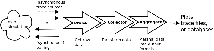
Data Collection Framework overview
The overall flow of data processing is depicted in Data Collection Framework overview. On the left side, a running ns-3 simulation is depicted. In the course of running the simulation, data is made available by models through trace sources, or via other means. The diagram depicts that probes can be connected to these trace sources to receive data asynchronously, or probes can poll for data. Data is then passed to a collector object that transforms the data. Finally, an aggregator can be connected to the outputs of the collector, to generate plots, files, or databases.
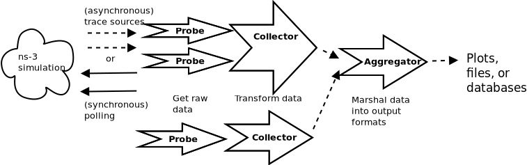
Data Collection Framework aggregation
A variation on the above figure is provided in Data Collection Framework aggregation. This second figure illustrates that the DCF objects may be chained together in a manner that downstream objects take inputs from multiple upstream objects. The figure conceptually shows that multiple probes may generate output that is fed into a single collector; as an example, a collector that outputs a ratio of two counters would typically acquire each counter data from separate probes. Multiple collectors can also feed into a single aggregator, which (as its name implies) may collect a number of data streams for inclusion into a single plot, file, or database.
3.4.2. Data Collection Helpers
The full flexibility of the data collection framework is provided by the interconnection of probes, collectors, and aggregators. Performing all of these interconnections leads to many configuration statements in user programs. For ease of use, some of the most common operations can be combined and encapsulated in helper functions. In addition, some statements involving ns-3 trace sources do not have Python bindings, due to limitations in the bindings.
3.4.2.1. Data Collection Helpers Overview
In this section, we provide an overview of some helper classes that have been created to ease the configuration of the data collection framework for some common use cases. The helpers allow users to form common operations with only a few statements in their C++ or Python programs. But, this ease of use comes at the cost of significantly less flexibility than low-level configuration can provide, and the need to explicitly code support for new Probe types into the helpers (to work around an issue described below).
The emphasis on the current helpers is to marshal data out of ns-3 trace sources into gnuplot plots or text files, without a high degree of output customization or statistical processing (initially). Also, the use is constrained to the available probe types in ns-3. Later sections of this documentation will go into more detail about creating new Probe types, as well as details about hooking together Probes, Collectors, and Aggregators in custom arrangements.
To date, two Data Collection helpers have been implemented:
GnuplotHelper
FileHelper
3.4.2.2. GnuplotHelper
The GnuplotHelper is a helper class for producing output files used to make gnuplots. The overall goal is to provide the ability for users to quickly make plots from data exported in ns-3 trace sources. By default, a minimal amount of data transformation is performed; the objective is to generate plots with as few (default) configuration statements as possible.
3.4.2.2.1. GnuplotHelper Overview
The GnuplotHelper will create 3 different files at the end of the simulation:
A space separated gnuplot data file
A gnuplot control file
A shell script to generate the gnuplot
There are two configuration statements that are needed to produce plots. The first statement configures the plot (filename, title, legends, and output type, where the output type defaults to PNG if unspecified):
void ConfigurePlot(const std::string &outputFileNameWithoutExtension,
                   const std::string &title,
                   const std::string &xLegend,
                   const std::string &yLegend,
                   const std::string &terminalType = ".png");
The second statement hooks the trace source of interest:
void PlotProbe(const std::string &typeId,
               const std::string &path,
               const std::string &probeTraceSource,
               const std::string &title);
The arguments are as follows:
typeId: The ns-3 TypeId of the Probe
path: The path in the ns-3 configuration namespace to one or more trace sources
probeTraceSource: Which output of the probe (itself a trace source) should be plotted
title: The title to associate with the dataset(s) (in the gnuplot legend)
A variant on the PlotProbe above is to specify a fifth optional argument that controls where in the plot the key (legend) is placed.
A fully worked example (from seventh.cc) is shown below:
// Create the gnuplot helper.
GnuplotHelper plotHelper;

// Configure the plot.
// Configure the plot.  The first argument is the file name prefix
// for the output files generated.  The second, third, and fourth
// arguments are, respectively, the plot title, x-axis, and y-axis labels
plotHelper.ConfigurePlot("seventh-packet-byte-count",
                         "Packet Byte Count vs. Time",
                         "Time(Seconds)",
                         "Packet Byte Count",
                         "png");

// Specify the probe type, trace source path (in configuration namespace), and
// probe output trace source ("OutputBytes") to plot.  The fourth argument
// specifies the name of the data series label on the plot.  The last
// argument formats the plot by specifying where the key should be placed.
plotHelper.PlotProbe(probeType,
                     tracePath,
                     "OutputBytes",
                     "Packet Byte Count",
                     GnuplotAggregator::KEY_BELOW);
In this example, the probeType and tracePath are as follows (for IPv4):
probeType = "ns3::Ipv4PacketProbe";
tracePath = "/NodeList/*/$ns3::Ipv4L3Protocol/Tx";
The probeType is a key parameter for this helper to work. This TypeId
must be registered in the system, and the signature on the Probe’s trace
sink must match that of the trace source it is being hooked to. Probe
types are pre-defined for a number of data types corresponding to ns-3
traced values, and for a few other trace source signatures such as the
‘Tx’ trace source of ns3::Ipv4L3Protocol class.
Note that the trace source path specified may contain wildcards. In this case, multiple datasets are plotted on one plot; one for each matched path.
The main output produced will be three files:
seventh-packet-byte-count.dat
seventh-packet-byte-count.plt
seventh-packet-byte-count.sh
At this point, users can either hand edit the .plt file for further customizations, or just run it through gnuplot. Running sh seventh-packet-byte-count.sh simply runs the plot through gnuplot, as shown below.
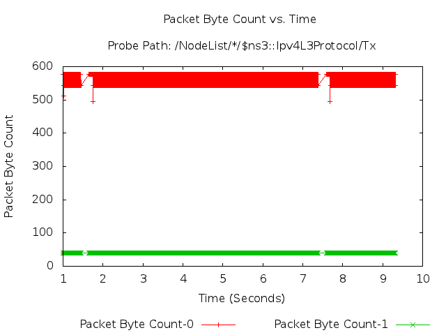
2-D Gnuplot Created by seventh.cc Example.
It can be seen that the key elements (legend, title, legend placement, xlabel, ylabel, and path for the data) are all placed on the plot. Since there were two matches to the configuration path provided, the two data series are shown:
Packet Byte Count-0 corresponds to /NodeList/0/$ns3::Ipv4L3Protocol/Tx
Packet Byte Count-1 corresponds to /NodeList/1/$ns3::Ipv4L3Protocol/Tx
3.4.2.2.2. GnuplotHelper ConfigurePlot
The GnuplotHelper’s ConfigurePlot() function can be used
to configure plots.
It has the following prototype:
void ConfigurePlot(const std::string &outputFileNameWithoutExtension,
                   const std::string &title,
                   const std::string &xLegend,
                   const std::string &yLegend,
                   const std::string &terminalType = ".png");
It has the following arguments:
Argument
Description
outputFileNameWithoutExtension
Name of gnuplot related files to write with no extension.
title
Plot title string to use for this plot.
xLegend
The legend for the x horizontal axis.
yLegend
The legend for the y vertical axis.
terminalType
Terminal type setting string for output. The default terminal type is “png”.
The GnuplotHelper’s ConfigurePlot() function configures plot
related parameters for this gnuplot helper so
that it will create a space separated gnuplot data file named
outputFileNameWithoutExtension + “.dat”, a gnuplot control file
named outputFileNameWithoutExtension + “.plt”, and a shell script
to generate the gnuplot named outputFileNameWithoutExtension +
“.sh”.
An example of how to use this function can be seen in the
seventh.cc code described above where it was used as follows:
plotHelper.ConfigurePlot("seventh-packet-byte-count",
                         "Packet Byte Count vs. Time",
                         "Time(Seconds)",
                         "Packet Byte Count",
                         "png");
3.4.2.2.3. GnuplotHelper PlotProbe
The GnuplotHelper’s PlotProbe() function can be used
to plot values generated by probes.
It has the following prototype:
void PlotProbe(const std::string &typeId,
               const std::string &path,
               const std::string &probeTraceSource,
               const std::string &title,
               enum GnuplotAggregator::KeyLocation keyLocation = GnuplotAggregator::KEY_INSIDE);
It has the following arguments:
Argument
Description
typeId
The type ID for the probe created by this helper.
path
Config path to access the trace source.
probeTraceSource
The probe trace source to access.
title
The title to be associated to this dataset
keyLocation
The location of the key in the plot. The default location is inside.
The GnuplotHelper’s PlotProbe() function
plots a dataset generated by hooking the ns-3 trace source with a
probe created by the helper, and then plotting the values from the
probeTraceSource.
The dataset will have the provided title, and will consist of
the ‘newValue’ at each timestamp.
If the config path has more than one match in the system because there is a wildcard, then one dataset for each match will be plotted. The dataset titles will be suffixed with the matched characters for each of the wildcards in the config path, separated by spaces. For example, if the proposed dataset title is the string “bytes”, and there are two wildcards in the path, then dataset titles like “bytes-0 0” or “bytes-12 9” will be possible as labels for the datasets that are plotted.
An example of how to use this function can be seen in the
seventh.cc code described above where it was used (with
variable substitution) as follows:
plotHelper.PlotProbe("ns3::Ipv4PacketProbe",
                     "/NodeList/*/$ns3::Ipv4L3Protocol/Tx",
                     "OutputBytes",
                     "Packet Byte Count",
                     GnuplotAggregator::KEY_BELOW);
3.4.2.2.4. Other Examples
A slightly simpler example than the seventh.cc example can be
found in src/stats/examples/gnuplot-helper-example.cc. The
following 2-D gnuplot was created using the example.
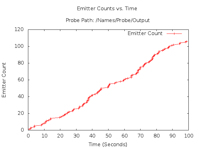
2-D Gnuplot Created by gnuplot-helper-example.cc Example.
In this example, there is an Emitter object that increments its counter according to a Poisson process and then emits the counter’s value as a trace source.
Ptr<Emitter> emitter = CreateObject<Emitter>();
Names::Add("/Names/Emitter", emitter);
Note that because there are no wildcards in the path used below, only 1 datastream was drawn in the plot. This single datastream in the plot is simply labeled “Emitter Count”, with no extra suffixes like one would see if there were wildcards in the path.
// Create the gnuplot helper.
GnuplotHelper plotHelper;

// Configure the plot.
plotHelper.ConfigurePlot("gnuplot-helper-example",
                         "Emitter Counts vs. Time",
                         "Time(Seconds)",
                         "Emitter Count",
                         "png");

// Plot the values generated by the probe.  The path that we provide
// helps to disambiguate the source of the trace.
plotHelper.PlotProbe("ns3::Uinteger32Probe",
                     "/Names/Emitter/Counter",
                     "Output",
                     "Emitter Count",
                     GnuplotAggregator::KEY_INSIDE);
3.4.2.3. FileHelper
The FileHelper is a helper class used to put data values into a file. The overall goal is to provide the ability for users to quickly make formatted text files from data exported in ns-3 trace sources. By default, a minimal amount of data transformation is performed; the objective is to generate files with as few (default) configuration statements as possible.
3.4.2.3.1. FileHelper Overview
The FileHelper will create 1 or more text files at the end of the simulation.
The FileHelper can create 4 different types of text files:
Formatted
Space separated (the default)
Comma separated
Tab separated
Formatted files use C-style format strings and the sprintf() function to print their values in the file being written.
The following text file with 2 columns of formatted values named
seventh-packet-byte-count-0.txt was created using more new
code that was added to the original ns-3 Tutorial example’s code.
Only the first 10 lines of this file are shown here for brevity.
Time (Seconds) = 1.000e+00    Packet Byte Count = 40
Time (Seconds) = 1.004e+00    Packet Byte Count = 40
Time (Seconds) = 1.004e+00    Packet Byte Count = 576
Time (Seconds) = 1.009e+00    Packet Byte Count = 576
Time (Seconds) = 1.009e+00    Packet Byte Count = 576
Time (Seconds) = 1.015e+00    Packet Byte Count = 512
Time (Seconds) = 1.017e+00    Packet Byte Count = 576
Time (Seconds) = 1.017e+00    Packet Byte Count = 544
Time (Seconds) = 1.025e+00    Packet Byte Count = 576
Time (Seconds) = 1.025e+00    Packet Byte Count = 544

...
The following different text file with 2 columns of formatted
values named seventh-packet-byte-count-1.txt was also
created using the same new code that was added to the original
ns-3 Tutorial example’s code. Only the first 10 lines of this
file are shown here for brevity.
Time (Seconds) = 1.002e+00    Packet Byte Count = 40
Time (Seconds) = 1.007e+00    Packet Byte Count = 40
Time (Seconds) = 1.013e+00    Packet Byte Count = 40
Time (Seconds) = 1.020e+00    Packet Byte Count = 40
Time (Seconds) = 1.028e+00    Packet Byte Count = 40
Time (Seconds) = 1.036e+00    Packet Byte Count = 40
Time (Seconds) = 1.045e+00    Packet Byte Count = 40
Time (Seconds) = 1.053e+00    Packet Byte Count = 40
Time (Seconds) = 1.061e+00    Packet Byte Count = 40
Time (Seconds) = 1.069e+00    Packet Byte Count = 40

...
The new code that was added to produce the two text files is below. More details about this API will be covered in a later section.
Note that because there were 2 matches for the wildcard in the path,
2 separate text files were created. The first text file, which is
named “seventh-packet-byte-count-0.txt”, corresponds to the
wildcard match with the “*” replaced with “0”. The second text file,
which is named “seventh-packet-byte-count-1.txt”, corresponds to
the wildcard match with the “*” replaced with “1”. Also, note that
the function call to WriteProbe() will give an error message if
there are no matches for a path that contains wildcards.
// Create the file helper.
FileHelper fileHelper;

// Configure the file to be written.
fileHelper.ConfigureFile("seventh-packet-byte-count",
                         FileAggregator::FORMATTED);

// Set the labels for this formatted output file.
fileHelper.Set2dFormat("Time (Seconds) = %.3e\tPacket Byte Count = %.0f");

// Write the values generated by the probe.
fileHelper.WriteProbe("ns3::Ipv4PacketProbe",
                      "/NodeList/*/$ns3::Ipv4L3Protocol/Tx",
                      "OutputBytes");
3.4.2.3.2. FileHelper ConfigureFile
The FileHelper’s ConfigureFile() function can be used
to configure text files.
It has the following prototype:
void ConfigureFile(const std::string &outputFileNameWithoutExtension,
                   enum FileAggregator::FileType fileType = FileAggregator::SPACE_SEPARATED);
It has the following arguments:
Argument
Description
outputFileNameWithoutExtension
Name of output file to write with no extension.
fileType
Type of file to write. The default type of file is space separated.
The FileHelper’s ConfigureFile() function configures text file
related parameters for the file helper so that
it will create a file named outputFileNameWithoutExtension plus
possible extra information from wildcard matches plus “.txt” with
values printed as specified by fileType. The default file type
is space-separated.
An example of how to use this function can be seen in the
seventh.cc code described above where it was used as follows:
fileHelper.ConfigureFile("seventh-packet-byte-count",
                         FileAggregator::FORMATTED);
3.4.2.3.3. FileHelper WriteProbe
The FileHelper’s WriteProbe() function can be used
to write values generated by probes to text files.
It has the following prototype:
void WriteProbe(const std::string &typeId,
                const std::string &path,
                const std::string &probeTraceSource);
It has the following arguments:
Argument
Description
typeId
The type ID for the probe to be created.
path
Config path to access the trace source.
probeTraceSource
The probe trace source to access.
The FileHelper’s WriteProbe() function
creates output text files generated by hooking the ns-3 trace source
with a probe created by the helper, and then writing the values from the
probeTraceSource. The output file names will have the text stored
in the member variable m_outputFileNameWithoutExtension plus “.txt”,
and will consist of the ‘newValue’ at each timestamp.
If the config path has more than one match in the system because there is a wildcard, then one output file for each match will be created. The output file names will contain the text in m_outputFileNameWithoutExtension plus the matched characters for each of the wildcards in the config path, separated by dashes, plus “.txt”. For example, if the value in m_outputFileNameWithoutExtension is the string “packet-byte-count”, and there are two wildcards in the path, then output file names like “packet-byte-count-0-0.txt” or “packet-byte-count-12-9.txt” will be possible as names for the files that will be created.
An example of how to use this function can be seen in the
seventh.cc code described above where it was used as follows:
fileHelper.WriteProbe("ns3::Ipv4PacketProbe",
                      "/NodeList/*/$ns3::Ipv4L3Protocol/Tx",
                      "OutputBytes");
3.4.2.3.4. Other Examples
A slightly simpler example than the seventh.cc example can be
found in src/stats/examples/file-helper-example.cc.
This example only uses the FileHelper.
The following text file with 2 columns of formatted values named
file-helper-example.txt was created using the example.
Only the first 10 lines of this file are shown here for brevity.
Time (Seconds) = 0.203  Count = 1
Time (Seconds) = 0.702  Count = 2
Time (Seconds) = 1.404  Count = 3
Time (Seconds) = 2.368  Count = 4
Time (Seconds) = 3.364  Count = 5
Time (Seconds) = 3.579  Count = 6
Time (Seconds) = 5.873  Count = 7
Time (Seconds) = 6.410  Count = 8
Time (Seconds) = 6.472  Count = 9
...
In this example, there is an Emitter object that increments its counter according to a Poisson process and then emits the counter’s value as a trace source.
Ptr<Emitter> emitter = CreateObject<Emitter>();
Names::Add("/Names/Emitter", emitter);
Note that because there are no wildcards in the path used below, only 1 text file was created. This single text file is simply named “file-helper-example.txt”, with no extra suffixes like you would see if there were wildcards in the path.
// Create the file helper.
FileHelper fileHelper;

// Configure the file to be written.
fileHelper.ConfigureFile("file-helper-example",
                         FileAggregator::FORMATTED);

// Set the labels for this formatted output file.
fileHelper.Set2dFormat("Time (Seconds) = %.3e\tCount = %.0f");

// Write the values generated by the probe.  The path that we
// provide helps to disambiguate the source of the trace.
fileHelper.WriteProbe("ns3::Uinteger32Probe",
                      "/Names/Emitter/Counter",
                      "Output");
3.4.2.4. Scope and Limitations
Currently, only these Probes have been implemented and connected to the GnuplotHelper and to the FileHelper:
BooleanProbe
DoubleProbe
Uinteger8Probe
Uinteger16Probe
Uinteger32Probe
TimeProbe
PacketProbe
ApplicationPacketProbe
Ipv4PacketProbe
These Probes, therefore, are the only TypeIds available to be used
in PlotProbe() and WriteProbe().
In the next few sections, we cover each of the fundamental object types (Probe, Collector, and Aggregator) in more detail, and show how they can be connected together using lower-level API.
3.4.3. Probes
This section details the functionalities provided by the Probe class to an ns-3 simulation, and gives examples on how to code them in a program. This section is meant for users interested in developing simulations with the ns-3 tools and using the Data Collection Framework, of which the Probe class is a part, to generate data output with their simulation’s results.
3.4.3.1. Probe Overview
A Probe object is supposed to be connected to a variable from the simulation whose values throughout the experiment are relevant to the user. The Probe will record what were values assumed by the variable throughout the simulation and pass such data to another member of the Data Collection Framework. While it is out of this section’s scope to discuss what happens after the Probe produces its output, it is sufficient to say that, by the end of the simulation, the user will have detailed information about what values were stored inside the variable being probed during the simulation.
Typically, a Probe is connected to an ns-3 trace source. In this manner, whenever the trace source exports a new value, the Probe consumes the value (and exports it downstream to another object via its own trace source).
The Probe can be thought of as kind of a filter on trace sources. The main reasons for possibly hooking to a Probe rather than directly to a trace source are as follows:
Probes may be dynamically turned on and off during the simulation with calls to
Enable()andDisable(). For example, the outputting of data may be turned off during the simulation warmup phase.Probes may perform operations on the data to extract values from more complicated structures; for instance, outputting the packet size value from a received ns3::Packet.
Probes register a name in the ns3::Config namespace (using
Names::Add()) so that other objects may refer to them.Probes provide a static method that allows one to manipulate a Probe by name, such as what is done in ns2measure [Cic06]
Stat::put("my_metric", ID, sample);
The ns-3 equivalent of the above ns2measure code is, e.g.
DoubleProbe::SetValueByPath("/path/to/probe", sample);
3.4.3.1.1. Creation
Note that a Probe base class object can not be created because it is an abstract base class, i.e. it has pure virtual functions that have not been implemented. An object of type DoubleProbe, which is a subclass of the Probe class, will be created here to show what needs to be done.
One declares a DoubleProbe in dynamic memory by using the smart pointer class
(Ptr<T>). To create a DoubleProbe in dynamic memory with smart pointers, one
just needs to call the ns-3 method CreateObject():
Ptr<DoubleProbe> myprobe = CreateObject<DoubleProbe>();
The declaration above creates DoubleProbes using the default values for its attributes. There are four attributes in the DoubleProbe class; two in the base class object DataCollectionObject, and two in the Probe base class:
“Name” (DataCollectionObject), a StringValue
“Enabled” (DataCollectionObject), a BooleanValue
“Start” (Probe), a TimeValue
“Stop” (Probe), a TimeValue
One can set such attributes at object creation by using the following method:
Ptr<DoubleProbe> myprobe = CreateObjectWithAttributes<DoubleProbe>(
    "Name", StringValue("myprobe"),
    "Enabled", BooleanValue(false),
    "Start", TimeValue(Seconds(100)),
    "Stop", TimeValue(Seconds(1000)));
Start and Stop are Time variables which determine the interval of action of the Probe. The Probe will only output data if the current time of the Simulation is inside of that interval. The special time value of 0 seconds for Stop will disable this attribute (i.e. keep the Probe on for the whole simulation). Enabled is a flag that turns the Probe on or off, and must be set to true for the Probe to export data. The Name is the object’s name in the DCF framework.
3.4.3.1.2. Importing and exporting data
ns-3 trace sources are strongly typed, so the mechanisms for hooking Probes to a trace source and for exporting data belong to its subclasses. For instance, the default distribution of ns-3 provides a class DoubleProbe that is designed to hook to a trace source exporting a double value. We’ll next detail the operation of the DoubleProbe, and then discuss how other Probe classes may be defined by the user.
3.4.3.2. DoubleProbe Overview
The DoubleProbe connects to a double-valued ns-3 trace source, and itself exports a different double-valued ns-3 trace source.
The following code, drawn from
src/stats/examples/double-probe-example.cc, shows the basic
operations of plumbing the DoubleProbe into a simulation, where it is
probing a Counter exported by an emitter object (class Emitter).
Ptr<Emitter> emitter = CreateObject<Emitter>();
Names::Add("/Names/Emitter", emitter);
...

Ptr<DoubleProbe> probe1 = CreateObject<DoubleProbe>();

// Connect the probe to the emitter's Counter
bool connected = probe1->ConnectByObject("Counter", emitter);
The following code is probing the same Counter exported by the same emitter object. This DoubleProbe, however, is using a path in the configuration namespace to make the connection. Note that the emitter registered itself in the configuration namespace after it was created; otherwise, the ConnectByPath would not work.
Ptr<DoubleProbe> probe2 = CreateObject<DoubleProbe>();

// Note, no return value is checked here
probe2->ConnectByPath("/Names/Emitter/Counter");
The next DoubleProbe shown that is shown below will have its value set using its path in the configuration namespace. Note that this time the DoubleProbe registered itself in the configuration namespace after it was created.
Ptr<DoubleProbe> probe3 = CreateObject<DoubleProbe>();
probe3->SetName("StaticallyAccessedProbe");

// We must add it to the config database
Names::Add("/Names/Probes", probe3->GetName(), probe3);
The emitter’s Count() function is now able to set the value for this DoubleProbe as follows:
void
Emitter::Count()
{
  ...
  m_counter += 1.0;
  DoubleProbe::SetValueByPath("/Names/StaticallyAccessedProbe", m_counter);
  ...
}
The above example shows how the code calling the Probe does not have to have an explicit reference to the Probe, but can direct the value setting through the Config namespace. This is similar in functionality to the Stat::Put method introduced by ns2measure paper [Cic06], and allows users to temporarily insert Probe statements like printf statements within existing ns-3 models. Note that in order to be able to use the DoubleProbe in this example like this, 2 things were necessary:
the stats module header file was included in the example .cc file
the example was made dependent on the stats module in its CMakeLists.txt file.
Analogous things need to be done in order to add other Probes in other places in the ns-3 code base.
The values for the DoubleProbe can also be set using the function DoubleProbe::SetValue(), while the values for the DoubleProbe can be gotten using the function DoubleProbe::GetValue().
The DoubleProbe exports double values in its “Output” trace source; a downstream object can hook a trace sink (NotifyViaProbe) to this as follows:
connected = probe1->TraceConnect("Output", probe1->GetName(), MakeCallback(&NotifyViaProbe));
3.4.3.3. Other probes
Besides the DoubleProbe, the following Probes are also available:
Uinteger8Probe connects to an ns-3 trace source exporting an uint8_t.
Uinteger16Probe connects to an ns-3 trace source exporting an uint16_t.
Uinteger32Probe connects to an ns-3 trace source exporting an uint32_t.
PacketProbe connects to an ns-3 trace source exporting a packet.
ApplicationPacketProbe connects to an ns-3 trace source exporting a packet and a socket address.
Ipv4PacketProbe connects to an ns-3 trace source exporting a packet, an IPv4 object, and an interface.
3.4.3.4. Creating new Probe types
To create a new Probe type, you need to perform the following steps:
Be sure that your new Probe class is derived from the Probe base class.
Be sure that the pure virtual functions that your new Probe class inherits from the Probe base class are implemented.
Find an existing Probe class that uses a trace source that is closest in type to the type of trace source your Probe will be using.
Copy that existing Probe class’s header file (.h) and implementation file (.cc) to two new files with names matching your new Probe.
Replace the types, arguments, and variables in the copied files with the appropriate type for your Probe.
Make necessary modifications to make the code compile and to make it behave as you would like.
3.4.3.5. Examples
Two examples will be discussed in detail here:
Double Probe Example
IPv4 Packet Plot Example
3.4.3.5.1. Double Probe Example
The double probe example has been discussed previously. The example
program can be found in
src/stats/examples/double-probe-example.cc. To
summarize what occurs in this program, there is an emitter that
exports a counter that increments according to a Poisson process. In
particular, two ways of emitting data are shown:
through a traced variable hooked to one Probe:
TracedValue<double> m_counter; // normally this would be integer type
through a counter whose value is posted to a second Probe, referenced by its name in the Config system:
void
Emitter::Count()
{
  NS_LOG_FUNCTION(this);
  NS_LOG_DEBUG("Counting at " << Simulator::Now().GetSeconds());
  m_counter += 1.0;
  DoubleProbe::SetValueByPath("/Names/StaticallyAccessedProbe", m_counter);
  Simulator::Schedule(Seconds(m_var->GetValue()), &Emitter::Count, this);
}
Let’s look at the Probe more carefully. Probes can receive their values in a multiple ways:
by the Probe accessing the trace source directly and connecting a trace sink to it
by the Probe accessing the trace source through the config namespace and connecting a trace sink to it
by the calling code explicitly calling the Probe’s SetValue() method
by the calling code explicitly calling SetValueByPath (“/path/through/Config/namespace”, …)
The first two techniques are expected to be the most common. Also in the example, the hooking of a normal callback function is shown, as is typically done in ns-3. This callback function is not associated with a Probe object. We’ll call this case 0) below.
// This is a function to test hooking a raw function to the trace source
void
NotifyViaTraceSource(std::string context, double oldVal, double newVal)
{
  NS_LOG_DEBUG("context: " << context << " old " << oldVal << " new " << newVal);
}
First, the emitter needs to be setup:
Ptr<Emitter> emitter = CreateObject<Emitter>();
Names::Add("/Names/Emitter", emitter);

// The Emitter object is not associated with an ns-3 node, so
// it won't get started automatically, so we need to do this ourselves
Simulator::Schedule(Seconds(0), &Emitter::Start, emitter);
The various DoubleProbes interact with the emitter in the example as shown below.
Case 0):
// The below shows typical functionality without a probe
// (connect a sink function to a trace source)
//
connected = emitter->TraceConnect("Counter", "sample context", MakeCallback(&NotifyViaTraceSource));
NS_ASSERT_MSG(connected, "Trace source not connected");
case 1):
//
// Probe1 will be hooked directly to the Emitter trace source object
//

// probe1 will be hooked to the Emitter trace source
Ptr<DoubleProbe> probe1 = CreateObject<DoubleProbe>();
// the probe's name can serve as its context in the tracing
probe1->SetName("ObjectProbe");

// Connect the probe to the emitter's Counter
connected = probe1->ConnectByObject("Counter", emitter);
NS_ASSERT_MSG(connected, "Trace source not connected to probe1");
case 2):
//
// Probe2 will be hooked to the Emitter trace source object by
// accessing it by path name in the Config database
//

// Create another similar probe; this will hook up via a Config path
Ptr<DoubleProbe> probe2 = CreateObject<DoubleProbe>();
probe2->SetName("PathProbe");

// Note, no return value is checked here
probe2->ConnectByPath("/Names/Emitter/Counter");
case 4)(case 3 is not shown in this example):
//
// Probe3 will be called by the emitter directly through the
// static method SetValueByPath().
//
Ptr<DoubleProbe> probe3 = CreateObject<DoubleProbe>();
probe3->SetName("StaticallyAccessedProbe");
// We must add it to the config database
Names::Add("/Names/Probes", probe3->GetName(), probe3);
And finally, the example shows how the probes can be hooked to generate output:
// The probe itself should generate output.  The context that we provide
// to this probe (in this case, the probe name) will help to disambiguate
// the source of the trace
connected = probe3->TraceConnect("Output",
                                 "/Names/Probes/StaticallyAccessedProbe/Output",
                                 MakeCallback(&NotifyViaProbe));
NS_ASSERT_MSG(connected, "Trace source not .. connected to probe3 Output");
The following callback is hooked to the Probe in this example for illustrative purposes; normally, the Probe would be hooked to a Collector object.
// This is a function to test hooking it to the probe output
void
NotifyViaProbe(std::string context, double oldVal, double newVal)
{
  NS_LOG_DEBUG("context: " << context << " old " << oldVal << " new " << newVal);
}
3.4.3.5.2. IPv4 Packet Plot Example
The IPv4 packet plot example is based on the fifth.cc example from the ns-3
Tutorial. It can be found in
src/stats/examples/ipv4-packet-plot-example.cc.
      node 0                 node 1
+----------------+    +----------------+
|    ns-3 TCP    |    |    ns-3 TCP    |
+----------------+    +----------------+
|    10.1.1.1    |    |    10.1.1.2    |
+----------------+    +----------------+
| point-to-point |    | point-to-point |
+----------------+    +----------------+
        |                     |
        +---------------------+
We’ll just look at the Probe, as it illustrates that Probes may also unpack values from structures (in this case, packets) and report those values as trace source outputs, rather than just passing through the same type of data.
There are other aspects of this example that will be explained later in the documentation. The two types of data that are exported are the packet itself (Output) and a count of the number of bytes in the packet (OutputBytes).
TypeId
Ipv4PacketProbe::GetTypeId()
{
  static TypeId tid = TypeId("ns3::Ipv4PacketProbe")
    .SetParent<Probe>()
    .AddConstructor<Ipv4PacketProbe>()
    .AddTraceSource( "Output",
                     "The packet plus its IPv4 object and interface that serve as the output for this probe",
                     MakeTraceSourceAccessor(&Ipv4PacketProbe::m_output))
    .AddTraceSource( "OutputBytes",
                     "The number of bytes in the packet",
                     MakeTraceSourceAccessor(&Ipv4PacketProbe::m_outputBytes))
  ;
  return tid;
}
When the Probe’s trace sink gets a packet, if the Probe is enabled, then it will output the packet on its Output trace source, but it will also output the number of bytes on the OutputBytes trace source.
void
Ipv4PacketProbe::TraceSink(Ptr<const Packet> packet, Ptr<Ipv4> ipv4, uint32_t interface)
{
  NS_LOG_FUNCTION(this << packet << ipv4 << interface);
  if (IsEnabled())
    {
      m_packet    = packet;
      m_ipv4      = ipv4;
      m_interface = interface;
      m_output(packet, ipv4, interface);

      uint32_t packetSizeNew = packet->GetSize();
      m_outputBytes(m_packetSizeOld, packetSizeNew);
      m_packetSizeOld = packetSizeNew;
    }
}
3.4.4. Collectors
This section is a placeholder to detail the functionalities provided by the Collector class to an ns-3 simulation, and gives examples on how to code them in a program.
Note: As of ns-3.18, Collectors are still under development and not yet provided as part of the framework.
3.4.5. Aggregators
This section details the functionalities provided by the Aggregator class to an ns-3 simulation. This section is meant for users interested in developing simulations with the ns-3 tools and using the Data Collection Framework, of which the Aggregator class is a part, to generate data output with their simulation’s results.
3.4.5.1. Aggregator Overview
An Aggregator object is supposed to be hooked to one or more trace sources in order to receive input. Aggregators are the end point of the data collected by the network of Probes and Collectors during the simulation. It is the Aggregator’s job to take these values and transform them into their final output format such as plain text files, spreadsheet files, plots, or databases.
Typically, an aggregator is connected to one or more Collectors. In this manner, whenever the Collectors’ trace sources export new values, the Aggregator can process the value so that it can be used in the final output format where the data values will reside after the simulation.
Note the following about Aggregators:
Aggregators may be dynamically turned on and off during the simulation with calls to
Enable()andDisable(). For example, the aggregating of data may be turned off during the simulation warmup phase, which means those values won’t be included in the final output medium.Aggregators receive data from Collectors via callbacks. When a Collector is associated to an aggregator, a call to TraceConnect is made to establish the Aggregator’s trace sink method as a callback.
To date, two Aggregators have been implemented:
GnuplotAggregator
FileAggregator
3.4.5.2. GnuplotAggregator
The GnuplotAggregator produces output files used to make gnuplots.
The GnuplotAggregator will create 3 different files at the end of the simulation:
A space separated gnuplot data file
A gnuplot control file
A shell script to generate the gnuplot
3.4.5.2.1. Creation
An object of type GnuplotAggregator will be created here to show what needs to be done.
One declares a GnuplotAggregator in dynamic memory by using the smart
pointer class (Ptr<T>). To create a GnuplotAggregator in dynamic
memory with smart pointers, one just needs to call the ns-3 method
CreateObject(). The following code from
src/stats/examples/gnuplot-aggregator-example.cc shows
how to do this:
string fileNameWithoutExtension = "gnuplot-aggregator";

// Create an aggregator.
Ptr<GnuplotAggregator> aggregator =
  CreateObject<GnuplotAggregator>(fileNameWithoutExtension);
The first argument for the constructor, fileNameWithoutExtension, is the name of the gnuplot related files to write with no extension. This GnuplotAggregator will create a space separated gnuplot data file named “gnuplot-aggregator.dat”, a gnuplot control file named “gnuplot-aggregator.plt”, and a shell script to generate the gnuplot named + “gnuplot-aggregator.sh”.
The gnuplot that is created can have its key in 4 different locations:
No key
Key inside the plot (the default)
Key above the plot
Key below the plot
The following gnuplot key location enum values are allowed to specify the key’s position:
enum KeyLocation {
  NO_KEY,
  KEY_INSIDE,
  KEY_ABOVE,
  KEY_BELOW
};
If it was desired to have the key below rather than the default position of inside, then you could do the following.
aggregator->SetKeyLocation(GnuplotAggregator::KEY_BELOW);
3.4.5.2.2. Examples
One example will be discussed in detail here:
Gnuplot Aggregator Example
An example that exercises the GnuplotAggregator can be found in
src/stats/examples/gnuplot-aggregator-example.cc.
The following 2-D gnuplot was created using the example.
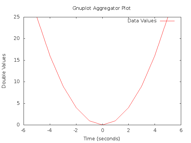
2-D Gnuplot Created by gnuplot-aggregator-example.cc Example.
This code from the example shows how to construct the GnuplotAggregator as was discussed above.
void Create2dPlot()
{
  std::string fileNameWithoutExtension = "gnuplot-aggregator";
  std::string plotTitle                = "Gnuplot Aggregator Plot";
  std::string plotXAxisHeading         = "Time(seconds)";
  std::string plotYAxisHeading         = "Double Values";
  std::string plotDatasetLabel         = "Data Values";
  std::string datasetContext           = "Dataset/Context/String";

  // Create an aggregator.
  Ptr<GnuplotAggregator> aggregator =
    CreateObject<GnuplotAggregator>(fileNameWithoutExtension);
Various GnuplotAggregator attributes are set including the 2-D dataset that will be plotted.
// Set the aggregator's properties.
aggregator->SetTerminal("png");
aggregator->SetTitle(plotTitle);
aggregator->SetLegend(plotXAxisHeading, plotYAxisHeading);

// Add a data set to the aggregator.
aggregator->Add2dDataset(datasetContext, plotDatasetLabel);

// aggregator must be turned on
aggregator->Enable();
Next, the 2-D values are calculated, and each one is individually
written to the GnuplotAggregator using the Write2d() function.
  double time;
  double value;

  // Create the 2-D dataset.
  for (time = -5.0; time <= +5.0; time += 1.0)
    {
      // Calculate the 2-D curve
      //
      //                   2
      //     value  =  time   .
      //
      value = time * time;

      // Add this point to the plot.
      aggregator->Write2d(datasetContext, time, value);
    }

  // Disable logging of data for the aggregator.
  aggregator->Disable();
}
3.4.5.3. FileAggregator
The FileAggregator sends the values it receives to a file.
The FileAggregator can create 4 different types of files:
Formatted
Space separated (the default)
Comma separated
Tab separated
Formatted files use C-style format strings and the sprintf() function to print their values in the file being written.
3.4.5.3.1. Creation
An object of type FileAggregator will be created here to show what needs to be done.
One declares a FileAggregator in dynamic memory by using the smart
pointer class (Ptr<T>). To create a FileAggregator in dynamic memory
with smart pointers, one just needs to call the ns-3 method
CreateObject. The following code from
src/stats/examples/file-aggregator-example.cc shows how
to do this:
string fileName       = "file-aggregator-formatted-values.txt";

// Create an aggregator that will have formatted values.
Ptr<FileAggregator> aggregator =
  CreateObject<FileAggregator>(fileName, FileAggregator::FORMATTED);
The first argument for the constructor, filename, is the name of the file to write; the second argument, fileType, is type of file to write. This FileAggregator will create a file named “file-aggregator-formatted-values.txt” with its values printed as specified by fileType, i.e., formatted in this case.
The following file type enum values are allowed:
enum FileType {
  FORMATTED,
  SPACE_SEPARATED,
  COMMA_SEPARATED,
  TAB_SEPARATED
};
3.4.5.3.2. Examples
One example will be discussed in detail here:
File Aggregator Example
An example that exercises the FileAggregator can be found in
src/stats/examples/file-aggregator-example.cc.
The following text file with 2 columns of values separated by commas was created using the example.
-5,25
-4,16
-3,9
-2,4
-1,1
0,0
1,1
2,4
3,9
4,16
5,25
This code from the example shows how to construct the FileAggregator as was discussed above.
void CreateCommaSeparatedFile()
{
  std::string fileName       = "file-aggregator-comma-separated.txt";
  std::string datasetContext = "Dataset/Context/String";

  // Create an aggregator.
  Ptr<FileAggregator> aggregator =
    CreateObject<FileAggregator>(fileName, FileAggregator::COMMA_SEPARATED);
FileAggregator attributes are set.
// aggregator must be turned on
aggregator->Enable();
Next, the 2-D values are calculated, and each one is individually
written to the FileAggregator using the Write2d() function.
  double time;
  double value;

  // Create the 2-D dataset.
  for (time = -5.0; time <= +5.0; time += 1.0)
    {
      // Calculate the 2-D curve
      //
      //                   2
      //     value  =  time   .
      //
      value = time * time;

      // Add this point to the plot.
      aggregator->Write2d(datasetContext, time, value);
    }

  // Disable logging of data for the aggregator.
  aggregator->Disable();
}
The following text file with 2 columns of formatted values was also created using the example.
Time = -5.000e+00  Value = 25
Time = -4.000e+00  Value = 16
Time = -3.000e+00  Value = 9
Time = -2.000e+00  Value = 4
Time = -1.000e+00  Value = 1
Time = 0.000e+00   Value = 0
Time = 1.000e+00   Value = 1
Time = 2.000e+00   Value = 4
Time = 3.000e+00   Value = 9
Time = 4.000e+00   Value = 16
Time = 5.000e+00   Value = 25
This code from the example shows how to construct the FileAggregator as was discussed above.
void CreateFormattedFile()
{
  std::string fileName       = "file-aggregator-formatted-values.txt";
  std::string datasetContext = "Dataset/Context/String";

  // Create an aggregator that will have formatted values.
  Ptr<FileAggregator> aggregator =
    CreateObject<FileAggregator>(fileName, FileAggregator::FORMATTED);
FileAggregator attributes are set, including the C-style format string to use.
// Set the format for the values.
aggregator->Set2dFormat("Time = %.3e\tValue = %.0f");

// aggregator must be turned on
aggregator->Enable();
Next, the 2-D values are calculated, and each one is individually
written to the FileAggregator using the Write2d() function.
  double time;
  double value;

  // Create the 2-D dataset.
  for (time = -5.0; time <= +5.0; time += 1.0)
    {
      // Calculate the 2-D curve
      //
      //                   2
      //     value  =  time   .
      //
      value = time * time;

      // Add this point to the plot.
      aggregator->Write2d(datasetContext, time, value);
    }

  // Disable logging of data for the aggregator.
  aggregator->Disable();
}
3.4.6. Adaptors
This section details the functionalities provided by the Adaptor class to an ns-3 simulation. This section is meant for users interested in developing simulations with the ns-3 tools and using the Data Collection Framework, of which the Adaptor class is a part, to generate data output with their simulation’s results.
Note: the term ‘adaptor’ may also be spelled ‘adapter’; we chose the spelling aligned with the C++ standard.
3.4.6.1. Adaptor Overview
An Adaptor is used to make connections between different types of DCF objects.
To date, one Adaptor has been implemented:
TimeSeriesAdaptor
3.4.6.2. Time Series Adaptor
The TimeSeriesAdaptor lets Probes connect directly to Aggregators without needing any Collector in between.
Both of the implemented DCF helpers utilize TimeSeriesAdaptors in order to take probed values of different types and output the current time plus the value with both converted to doubles.
The role of the TimeSeriesAdaptor class is that of an adaptor, which takes raw-valued probe data of different types and outputs a tuple of two double values. The first is a timestamp, which may be set to different resolutions (e.g. Seconds, Milliseconds, etc.) in the future but which is presently hardcoded to Seconds. The second is the conversion of a non-double value to a double value (possibly with loss of precision).
3.4.7. Scope/Limitations
This section discusses the scope and limitations of the Data Collection Framework.
Currently, only these Probes have been implemented in DCF:
BooleanProbe
DoubleProbe
Uinteger8Probe
Uinteger16Probe
Uinteger32Probe
TimeProbe
PacketProbe
ApplicationPacketProbe
Ipv4PacketProbe
Currently, no Collectors are available in the DCF, although a BasicStatsCollector is under development.
Currently, only these Aggregators have been implemented in DCF:
GnuplotAggregator
FileAggregator
Currently, only this Adaptor has been implemented in DCF:
Time-Series Adaptor.
3.4.7.1. Future Work
This section discusses the future work to be done on the Data Collection Framework.
Here are some things that still need to be done:
Hook up more trace sources in ns-3 code to get more values out of the simulator.
Implement more types of Probes than there currently are.
Implement more than just the single current 2-D Collector, BasicStatsCollector.
Implement more Aggregators.
Implement more than just Adaptors.
3.5. Statistical Framework
This chapter outlines work on simulation data collection and the statistical framework for ns-3.
The source code for the statistical framework lives in the directory
src/stats.
3.5.1. Goals
Primary objectives for this effort are the following:
Provide functionality to record, calculate, and present data and statistics for analysis of network simulations.
Boost simulation performance by reducing the need to generate extensive trace logs in order to collect data.
Enable simulation control via online statistics, e.g. terminating simulations or repeating trials.
Derived sub-goals and other target features include the following:
Integration with the existing ns-3 tracing system as the basic instrumentation framework of the internal simulation engine, e.g. network stacks, net devices, and channels.
Enabling users to utilize the statistics framework without requiring use of the tracing system.
Helping users create, aggregate, and analyze data over multiple trials.
Support for user created instrumentation, e.g. of application specific events and measures.
Low memory and CPU overhead when the package is not in use.
Leveraging existing analysis and output tools as much as possible. The framework may provide some basic statistics, but the focus is on collecting data and making it accessible for manipulation in established tools.
Eventual support for distributing independent replications is important but not included in the first round of features.
3.5.2. Overview
The statistics framework includes the following features:
The core framework and two basic data collectors: A counter, and a min/max/avg/total observer.
Extensions of those to easily work with times and packets.
Plaintext output formatted for OMNet++.
Database output using SQLite, a standalone, lightweight, high performance SQL engine.
Mandatory and open ended metadata for describing and working with runs.
An example based on the notional experiment of examining the properties of NS-3’s default ad hoc WiFi performance. It incorporates the following:
Constructs of a two node ad hoc WiFi network, with the nodes a parameterized distance apart.
UDP traffic source and sink applications with slightly different behavior and measurement hooks than the stock classes.
Data collection from the NS-3 core via existing trace signals, in particular data on frames transmitted and received by the WiFi MAC objects.
Instrumentation of custom applications by connecting new trace signals to the stat framework, as well as via direct updates. Information is recorded about total packets sent and received, bytes transmitted, and end-to-end delay.
An example of using packet tags to track end-to-end delay.
A simple control script which runs a number of trials of the experiment at varying distances and queries the resulting database to produce a graph using GNUPlot.
3.5.3. To-Do
High priority items include:
Inclusion of online statistics code, e.g. for memory efficient confidence intervals.
Provisions in the data collectors for terminating runs, i.e. when a threshold or confidence is met.
Data collectors for logging samples over time, and output to the various formats.
Demonstrate writing simple cyclic event glue to regularly poll some value.
Each of those should prove straightforward to incorporate in the current framework.
3.5.4. Approach
The framework is based around the following core principles:
One experiment trial is conducted by one instance of a simulation program, whether in parallel or serially.
A control script executes instances of the simulation, varying parameters as necessary.
Data is collected and stored for plotting and analysis using external scripts and existing tools.
Measures within the ns-3 core are taken by connecting the stat framework to existing trace signals.
Trace signals or direct manipulation of the framework may be used to instrument custom simulation code.
Those basic components of the framework and their interactions are depicted in the following figure.
3.5.5. Example
This section goes through the process of constructing an experiment in the framework and producing data for analysis (graphs) from it, demonstrating the structure and API along the way.
3.5.5.1. Question
‘’What is the (simulated) performance of ns-3’s WiFi NetDevices (using the default settings)? How far apart can wireless nodes be in a simulation before they cannot communicate reliably?’’
Hypothesis: Based on knowledge of real life performance, the nodes should communicate reasonably well to at least 100m apart. Communication beyond 200m shouldn’t be feasible.
Although not a very common question in simulation contexts, this is an important property of which simulation developers should have a basic understanding. It is also a common study done on live hardware.
3.5.5.2. Simulation Program
The first thing to do in implementing this experiment is developing the simulation program. The code for this example can be found in examples/stats/wifi-example-sim.cc. It does the following main steps.
Declaring parameters and parsing the command line using
ns3::CommandLine.double distance = 50.0; string format("OMNet++"); string experiment("wifi-distance-test"); string strategy("wifi-default"); string runID; CommandLine cmd(__FILE__); cmd.AddValue("distance", "Distance apart to place nodes(in meters).", distance); cmd.AddValue("format", "Format to use for data output.", format); cmd.AddValue("experiment", "Identifier for experiment.", experiment); cmd.AddValue("strategy", "Identifier for strategy.", strategy); cmd.AddValue("run", "Identifier for run.", runID); cmd.Parse(argc, argv);
Creating nodes and network stacks using
ns3::NodeContainer,ns3::WiFiHelper, andns3::InternetStackHelper.NodeContainer nodes; nodes.Create(2); WifiHelper wifi; wifi.SetMac("ns3::AdhocWifiMac"); wifi.SetPhy("ns3::WifiPhy"); NetDeviceContainer nodeDevices = wifi.Install(nodes); InternetStackHelper internet; internet.Install(nodes); Ipv4AddressHelper ipAddrs; ipAddrs.SetBase("192.168.0.0", "255.255.255.0"); ipAddrs.Assign(nodeDevices);
Positioning the nodes using
ns3::MobilityHelper. By default the nodes have static mobility and won’t move, but must be positioned the given distance apart. There are several ways to do this; it is done here usingns3::ListPositionAllocator, which draws positions from a given list.MobilityHelper mobility; Ptr<ListPositionAllocator> positionAlloc = CreateObject<ListPositionAllocator>(); positionAlloc->Add(Vector(0.0, 0.0, 0.0)); positionAlloc->Add(Vector(0.0, distance, 0.0)); mobility.SetPositionAllocator(positionAlloc); mobility.Install(nodes);
Installing a traffic generator and a traffic sink. The stock
Applicationscould be used, but the example includes custom objects insrc/test/test02-apps.(cc|h). These have a simple behavior, generating a given number of packets spaced at a given interval. As there is only one of each they are installed manually; for a larger set thens3::ApplicationHelperclass could be used. The commented-outConfig::Setline changes the destination of the packets, set to broadcast by default in this example. Note that in general WiFi may have different performance for broadcast and unicast frames due to different rate control and MAC retransmission policies.Ptr<Node> appSource = NodeList::GetNode(0); Ptr<Sender> sender = CreateObject<Sender>(); appSource->AddApplication(sender); sender->Start(Seconds(1)); Ptr<Node> appSink = NodeList::GetNode(1); Ptr<Receiver> receiver = CreateObject<Receiver>(); appSink->AddApplication(receiver); receiver->Start(Seconds(0)); // Config::Set("/NodeList/*/ApplicationList/*/$Sender/Destination", // Ipv4AddressValue("192.168.0.2"));
Configuring the data and statistics to be collected. The basic paradigm is that an
ns3::DataCollectorobject is created to hold information about this particular run, to which observers and calculators are attached to actually generate data. Importantly, run information includes labels for the ‘’experiment’’, ‘’strategy’’, ‘’input’’, and ‘’run’’. These are used to later identify and easily group data from multiple trials.The experiment is the study of which this trial is a member. Here it is on WiFi performance and distance.
The strategy is the code or parameters being examined in this trial. In this example it is fixed, but an obvious extension would be to investigate different WiFi bit rates, each of which would be a different strategy.
The input is the particular problem given to this trial. Here it is simply the distance between the two nodes.
The runID is a unique identifier for this trial with which it’s information is tagged for identification in later analysis. If no run ID is given the example program makes a (weak) run ID using the current time.
Those four pieces of metadata are required, but more may be desired. They may be added to the record using the
ns3::DataCollector::AddMetadata()method.DataCollector data; data.DescribeRun(experiment, strategy, input, runID); data.AddMetadata("author", "tjkopena");
Actual observation and calculating is done by
ns3::DataCalculatorobjects, of which several different types exist. These are created by the simulation program, attached to reporting or sampling code, and then registered with thens3::DataCollectorso they will be queried later for their output. One easy observation mechanism is to use existing trace sources, for example to instrument objects in the ns-3 core without changing their code. Here a counter is attached directly to a trace signal in the WiFi MAC layer on the target node.Ptr<PacketCounterCalculator> totalRx = CreateObject<PacketCounterCalculator>(); totalRx->SetKey("wifi-rx-frames"); Config::Connect("/NodeList/1/DeviceList/*/$ns3::WifiNetDevice/Rx", MakeCallback(&PacketCounterCalculator::FrameUpdate, totalRx)); data.AddDataCalculator(totalRx);
Calculators may also be manipulated directly. In this example, a counter is created and passed to the traffic sink application to be updated when packets are received.
Ptr<CounterCalculator<>> appRx = CreateObject<CounterCalculator<>>();
appRx->SetKey("receiver-rx-packets");
receiver->SetCounter(appRx);
data.AddDataCalculator(appRx);
To increment the count, the sink’s packet processing code then calls one of the calculator’s update methods.
m_calc->Update();
The program includes several other examples as well, using both the primitive calculators such as
ns3::CounterCalculatorand those adapted for observing packets and times. Insrc/test/test02-apps.(cc|h)it also creates a simple custom tag which it uses to track end-to-end delay for generated packets, reporting results to ans3::TimeMinMaxAvgTotalCalculatordata calculator.Running the simulation, which is very straightforward once constructed.
Simulator::Run();
Generating either OMNet++ or SQLite output, depending on the command line arguments. To do this a
ns3::DataOutputInterfaceobject is created and configured. The specific type of this will determine the output format. This object is then given thens3::DataCollectorobject which it interrogates to produce the output.Ptr<DataOutputInterface> output; if (format == "OMNet++") { NS_LOG_INFO("Creating OMNet++ formatted data output."); output = CreateObject<OmnetDataOutput>(); } else { # ifdef STAT_USE_DB NS_LOG_INFO("Creating SQLite formatted data output."); output = CreateObject<SqliteDataOutput>(); # endif } output->Output(data);
Freeing any memory used by the simulation. This should come at the end of the main function for the example.
Simulator::Destroy();
3.5.5.2.1. Logging
To see what the example program, applications, and stat framework are doing in detail, set the NS_LOG variable appropriately. The following will provide copious output from all three.
$ export NS_LOG=WiFiDistanceExperiment:WiFiDistanceApps
Note that this slows down the simulation extraordinarily.
3.5.5.2.2. Sample Output
Compiling and simply running the test program will append OMNet++ formatted output such as the following to data.sca.
run run-1212239121

attr experiment "wifi-distance-test"
attr strategy "wifi-default"
attr input "50"
attr description ""

attr "author" "tjkopena"

scalar wifi-tx-frames count 30
scalar wifi-rx-frames count 30
scalar sender-tx-packets count 30
scalar receiver-rx-packets count 30
scalar tx-pkt-size count 30
scalar tx-pkt-size total 1920
scalar tx-pkt-size average 64
scalar tx-pkt-size max 64
scalar tx-pkt-size min 64
scalar delay count 30
scalar delay total 5884980ns
scalar delay average 196166ns
scalar delay max 196166ns
scalar delay min 196166ns
3.5.5.3. Control Script
In order to automate data collection at a variety of inputs (distances), a simple Bash script is used to execute a series of simulations. It can be found at examples/stats/wifi-example-db.sh. The script is meant to be run from the examples/stats/ directory.
The script runs through a set of distances, collecting the results into an SQLite database. At each distance five trials are conducted to give a better picture of expected performance. The entire experiment takes only a few dozen seconds to run on a low end machine as there is no output during the simulation and little traffic is generated.
#!/bin/sh

DISTANCES="25 50 75 100 125 145 147 150 152 155 157 160 162 165 167 170 172 175 177 180"
TRIALS="1 2 3 4 5"

echo WiFi Experiment Example

if [ -e data.db ]
then
  echo Kill data.db?
  read ANS
  if [ "$ANS" = "yes" -o "$ANS" = "y" ]
  then
    echo Deleting database
    rm data.db
  fi
fi

for trial in $TRIALS
do
  for distance in $DISTANCES
  do
    echo Trial $trial, distance $distance
    ./bin/test02 --format=db --distance=$distance --run=run-$distance-$trial
  done
done
3.5.5.4. Analysis and Conclusion
Once all trials have been conducted, the script executes a simple SQL query over the database using the SQLite command line program. The query computes average packet loss in each set of trials associated with each distance. It does not take into account different strategies, but the information is present in the database to make some simple extensions and do so. The collected data is then passed to GNUPlot for graphing.
CMD="select exp.input,avg(100-((rx.value*100)/tx.value)) \
    from Singletons rx, Singletons tx, Experiments exp \
    where rx.run = tx.run AND \
          rx.run = exp.run AND \
          rx.name='receiver-rx-packets' AND \
          tx.name='sender-tx-packets' \
    group by exp.input \
    order by abs(exp.input) ASC;"

sqlite3 -noheader data.db "$CMD" > wifi-default.data
sed -i "s/|/   /" wifi-default.data
gnuplot wifi-example.gnuplot
The GNUPlot script found at examples/stats/wifi-example.gnuplot simply defines the output format and some basic formatting for the graph.
set terminal postscript portrait enhanced lw 2 "Helvetica" 14

set size 1.0, 0.66

#-------------------------------------------------------
set out "wifi-default.eps"
#set title "Packet Loss Over Distance"
set xlabel "Distance (m) --- average of 5 trials per point"
set xrange [0:200]
set ylabel "% Packet Loss"
set yrange [0:110]

plot "wifi-default.data" with lines title "WiFi Defaults"
3.5.5.4.1. End Result
The resulting graph provides no evidence that the default WiFi model’s performance is necessarily unreasonable and lends some confidence to an at least token faithfulness to reality. More importantly, this simple investigation has been carried all the way through using the statistical framework. Success!
3.6. Helpers
The above chapters introduced you to various ns-3 programming concepts such as smart pointers for reference-counted memory management, attributes, namespaces, callbacks, etc. Users who work at this low-level API can interconnect ns-3 objects with fine granularity. However, a simulation program written entirely using the low-level API would be quite long and tedious to code. For this reason, a separate so-called “helper API” has been overlaid on the core ns-3 API. If you have read the ns-3 tutorial, you will already be familiar with the helper API, since it is the API that new users are typically introduced to first. In this chapter, we introduce the design philosophy of the helper API and contrast it to the low-level API. If you become a heavy user of ns-3, you will likely move back and forth between these APIs even in the same program.
The helper API has a few goals:
the rest of
src/has no dependencies on the helper API; anything that can be done with the helper API can be coded also at the low-level APIContainers: Often simulations will need to do a number of identical actions to groups of objects. The helper API makes heavy use of containers of similar objects to which similar or identical operations can be performed.
The helper API is not generic; it does not strive to maximize code reuse. So, programming constructs such as polymorphism and templates that achieve code reuse are not as prevalent. For instance, there are separate
CsmaNetDevicehelpers andPointToPointNetDevicehelpers but they do not derive from a commonNetDevicebase class.The helper API typically works with stack-allocated (vs. heap-allocated) objects. For some programs, ns-3 users may not need to worry about any low level Object Create or Ptr handling; they can make do with containers of objects and stack-allocated helpers that operate on them.
The helper API is really all about making ns-3 programs easier to write and read, without taking away the power of the low-level interface. The rest of this chapter provides some examples of the programming conventions of the helper API.
3.7. Making Plots using the Gnuplot Class
There are 2 common methods to make a plot using ns-3 and gnuplot (http://www.gnuplot.info):
Create a gnuplot control file using ns-3’s Gnuplot class.
Create a gnuplot data file using values generated by ns-3.
This section is about method 1, i.e. it is about how to make a plot using ns-3’s Gnuplot class. If you are interested in method 2, see the “A Real Example” subsection under the “Tracing” section in the ns-3 Tutorial.
3.7.1. Creating Plots Using the Gnuplot Class
The following steps must be taken in order to create a plot using ns-3’s Gnuplot class:
Modify your code so that is uses the Gnuplot class and its functions.
Run your code so that it creates a gnuplot control file.
Call gnuplot with the name of the gnuplot control file.
View the graphics file that was produced in your favorite graphics viewer.
See the code from the example plots that are discussed below for details on step 1.
3.7.2. An Example Program that Uses the Gnuplot Class
An example program that uses ns-3’s Gnuplot class can be found here:
src/stats/examples/gnuplot-example.cc
In order to run this example, do the following:
$ ./ns3 run src/stats/examples/gnuplot-example
This should produce the following gnuplot control files:
plot-2d.plt
plot-2d-with-error-bars.plt
plot-3d.plt
In order to process these gnuplot control files, do the following:
$ gnuplot plot-2d.plt
$ gnuplot plot-2d-with-error-bars.plt
$ gnuplot plot-3d.plt
This should produce the following graphics files:
plot-2d.png
plot-2d-with-error-bars.png
plot-3d.png
You can view these graphics files in your favorite graphics viewer. If you have gimp installed on your machine, for example, you can do this:
$ gimp plot-2d.png
$ gimp plot-2d-with-error-bars.png
$ gimp plot-3d.png
3.7.3. An Example 2-Dimensional Plot
The following 2-Dimensional plot

was created using the following code from gnuplot-example.cc:
std::string fileNameWithNoExtension = "plot-2d";
std::string graphicsFileName        = fileNameWithNoExtension + ".png";
std::string plotFileName            = fileNameWithNoExtension + ".plt";
std::string plotTitle               = "2-D Plot";
std::string dataTitle               = "2-D Data";

// Instantiate the plot and set its title.
Gnuplot plot(graphicsFileName);
plot.SetTitle(plotTitle);

// Make the graphics file, which the plot file will create when it
// is used with Gnuplot, be a PNG file.
plot.SetTerminal("png");

// Set the labels for each axis.
plot.SetLegend("X Values", "Y Values");

// Set the range for the x axis.
plot.AppendExtra("set xrange [-6:+6]");

// Instantiate the dataset, set its title, and make the points be
// plotted along with connecting lines.
Gnuplot2dDataset dataset;
dataset.SetTitle(dataTitle);
dataset.SetStyle(Gnuplot2dDataset::LINES_POINTS);

double x;
double y;

// Create the 2-D dataset.
for (x = -5.0; x <= +5.0; x += 1.0)
  {
    // Calculate the 2-D curve
    //
    //            2
    //     y  =  x   .
    //
    y = x * x;

    // Add this point.
    dataset.Add(x, y);
  }

// Add the dataset to the plot.
plot.AddDataset(dataset);

// Open the plot file.
std::ofstream plotFile(plotFileName.c_str());

// Write the plot file.
plot.GenerateOutput(plotFile);

// Close the plot file.
plotFile.close();
3.7.4. An Example 2-Dimensional Plot with Error Bars
The following 2-Dimensional plot with error bars in the x and y directions
was created using the following code from gnuplot-example.cc:
std::string fileNameWithNoExtension = "plot-2d-with-error-bars";
std::string graphicsFileName        = fileNameWithNoExtension + ".png";
std::string plotFileName            = fileNameWithNoExtension + ".plt";
std::string plotTitle               = "2-D Plot With Error Bars";
std::string dataTitle               = "2-D Data With Error Bars";

// Instantiate the plot and set its title.
Gnuplot plot(graphicsFileName);
plot.SetTitle(plotTitle);

// Make the graphics file, which the plot file will create when it
// is used with Gnuplot, be a PNG file.
plot.SetTerminal("png");

// Set the labels for each axis.
plot.SetLegend("X Values", "Y Values");

// Set the range for the x axis.
plot.AppendExtra("set xrange [-6:+6]");

// Instantiate the dataset, set its title, and make the points be
// plotted with no connecting lines.
Gnuplot2dDataset dataset;
dataset.SetTitle(dataTitle);
dataset.SetStyle(Gnuplot2dDataset::POINTS);

// Make the dataset have error bars in both the x and y directions.
dataset.SetErrorBars(Gnuplot2dDataset::XY);

double x;
double xErrorDelta;
double y;
double yErrorDelta;

// Create the 2-D dataset.
for (x = -5.0; x <= +5.0; x += 1.0)
  {
    // Calculate the 2-D curve
    //
    //            2
    //     y  =  x   .
    //
    y = x * x;

    // Make the uncertainty in the x direction be constant and make
    // the uncertainty in the y direction be a constant fraction of
    // y's value.
    xErrorDelta = 0.25;
    yErrorDelta = 0.1 * y;

    // Add this point with uncertainties in both the x and y
    // direction.
    dataset.Add(x, y, xErrorDelta, yErrorDelta);
  }

// Add the dataset to the plot.
plot.AddDataset(dataset);

// Open the plot file.
std::ofstream plotFile(plotFileName.c_str());

// Write the plot file.
plot.GenerateOutput(plotFile);

// Close the plot file.
plotFile.close();
3.7.5. An Example 3-Dimensional Plot
The following 3-Dimensional plot

was created using the following code from gnuplot-example.cc:
std::string fileNameWithNoExtension = "plot-3d";
std::string graphicsFileName        = fileNameWithNoExtension + ".png";
std::string plotFileName            = fileNameWithNoExtension + ".plt";
std::string plotTitle               = "3-D Plot";
std::string dataTitle               = "3-D Data";

// Instantiate the plot and set its title.
Gnuplot plot(graphicsFileName);
plot.SetTitle(plotTitle);

// Make the graphics file, which the plot file will create when it
// is used with Gnuplot, be a PNG file.
plot.SetTerminal("png");

// Rotate the plot 30 degrees around the x axis and then rotate the
// plot 120 degrees around the new z axis.
plot.AppendExtra("set view 30, 120, 1.0, 1.0");

// Make the zero for the z-axis be in the x-axis and y-axis plane.
plot.AppendExtra("set ticslevel 0");

// Set the labels for each axis.
plot.AppendExtra("set xlabel 'X Values'");
plot.AppendExtra("set ylabel 'Y Values'");
plot.AppendExtra("set zlabel 'Z Values'");

// Set the ranges for the x and y axis.
plot.AppendExtra("set xrange [-5:+5]");
plot.AppendExtra("set yrange [-5:+5]");

// Instantiate the dataset, set its title, and make the points be
// connected by lines.
Gnuplot3dDataset dataset;
dataset.SetTitle(dataTitle);
dataset.SetStyle("with lines");

double x;
double y;
double z;

// Create the 3-D dataset.
for (x = -5.0; x <= +5.0; x += 1.0)
  {
    for (y = -5.0; y <= +5.0; y += 1.0)
      {
        // Calculate the 3-D surface
        //
        //            2      2
        //     z  =  x   *  y   .
        //
        z = x * x * y * y;

        // Add this point.
        dataset.Add(x, y, z);
      }

    // The blank line is necessary at the end of each x value's data
    // points for the 3-D surface grid to work.
    dataset.AddEmptyLine();
  }

// Add the dataset to the plot.
plot.AddDataset(dataset);

// Open the plot file.
std::ofstream plotFile(plotFileName.c_str());

// Write the plot file.
plot.GenerateOutput(plotFile);

// Close the plot file.
plotFile.close();
3.8. Using Python to Run ns-3
Python bindings allow the C++ code in ns-3 to be called from Python.
This chapter shows you how to create a Python script that can run ns-3 and also the process of creating Python bindings for a C++ ns-3 module.
Python bindings are also needed to run the Pyviz visualizer.
3.8.1. Introduction
Python bindings provide support for importing ns-3 model libraries as Python modules. Coverage of most of the ns-3 C++ API is provided. The intent has been to allow the programmer to write complete simulation scripts in Python, to allow integration of ns-3 with other Python tools and workflows. The intent is not to provide a different language choice to author new ns-3 models implemented in Python.
As of ns-3.37 release or later, Python bindings for ns-3 use a tool called Cppyy (https://cppyy.readthedocs.io/en/latest/) to create a Python module from the C++ libraries built by CMake. The Python bindings that Cppyy uses are built at runtime, by importing the C++ libraries and headers for each ns-3 module. This means that even if the C++ API changes, the Python bindings will adapt to them without requiring any preprocessing or scanning.
If a user is not interested in Python, no action is needed; the Python bindings are only built on-demand by Cppyy, and only if the user enables them in the configuration of ns-3.
Prior to ns-3.37, the previous Python bindings framework was based on Pybindgen.
3.8.2. Python virtual environment
According to PEP 668 it is a best practice to create a virtual environment for each new Python project. This isolates and simplifies dependency management. This is done via Python virtual environments (VENV).
Trying to pip install cppyy, required for ns-3 python bindings, system-wide will likely result in the following error message:
~$ pip install cppyy
error: externally-managed-environment

x This environment is externally managed
└─> To install Python packages system-wide, try apt install
    python3-xyz, where xyz is the package you are trying to
    install.

    If you wish to install a non-Debian-packaged Python package,
    create a virtual environment using python3 -m venv path/to/venv.
    Then use path/to/venv/bin/python and path/to/venv/bin/pip. Make
    sure you have python3-full installed.

    If you wish to install a non-Debian packaged Python application,
    it may be easiest to use pipx install xyz, which will manage a
    virtual environment for you. Make sure you have pipx installed.

    See /usr/share/doc/python3.12/README.venv for more information.

note: If you believe this is a mistake, please contact your Python
      installation or OS distribution provider. You can override this,
      at the risk of breaking your Python installation or OS, by
      passing --break-system-packages.
hint: See PEP 668 for the detailed specification.
While it is possible to ignore it via the --break-system-packages
that can cause packages required by your operating system to fail.
You can check this is actually the case by running pip freeze, which
will list multiple pip packages installed along the OS.
~$ pip freeze
...
ubuntu-pro-client==8001
...
Therefore, it is recommended you create a virtual environment and use it. This can be done with the following command:
~$ python3 -m venv myEnv
Note: if you don’t have venv installed, you will need to install it
either via the system package manager (e.g. apt install python3-venv),
or via pip itself (e.g. pip install venv).
After creating the venv, it is necessary to activate it, to properly set environment variables that will treat it as the active python installation.
~$ source ~/myEnv/bin/activate
(myEnv) ~$ whereis python
python: ~/myEnv/bin/python
(myEnv) ~$ pip freeze
(myEnv) ~$
From this point onwards, it is assumed all python commands are executed from within a virtual environment (venv).
Note: When configuring ns-3 python bindings from source, make sure to activate the venv before configuring. The appropriate Python venv will be passed to CMake for proper configuration and used by the ns-3 script to execute scripts. This includes python scripts called by C++ programs.
Important: Some pip packages can fail to install (for example, due to missing dependencies), as shown below. Their dependencies can typically be installed via the system package manager (apt, pacman, apk, etc).
It is also not uncommon for frequently used pip packages, such as pygraphviz, to be distributed
along with their dependencies via the system package manager (for example, python3-pygraphviz
in Debian-based distros).
However, a previously created venv will not detect pip packages installed via the package manager,
unless it is recreated with the --system-site-packages flag, as shown below. The drawback of this
approach is that all system packages will be exposed, which may lead to version conflicts with packages
you intend to use. If you use the pip freeze command to generate the requirements.txt list of dependencies
for your environment, unrelated system packages will also be included.
(myEnv) ~$ pip install pygraphviz
Collecting pygraphviz
  Using cached pygraphviz-1.14.tar.gz (106 kB)
  Installing build dependencies ... done
  Getting requirements to build wheel ... done
  Preparing metadata (pyproject.toml) ... done
Building wheels for collected packages: pygraphviz
  Building wheel for pygraphviz (pyproject.toml) ... error
  error: subprocess-exited-with-error

  | Building wheel for pygraphviz (pyproject.toml) did not run successfully.
  | exit code: 1
  --> running bdist_wheel
      running build
      running build_py
      creating build/lib.linux-x86_64-cpython-313/pygraphviz
      copying pygraphviz/testing.py -> build/lib.linux-x86_64-cpython-313/pygraphviz
      copying pygraphviz/scraper.py -> build/lib.linux-x86_64-cpython-313/pygraphviz
      copying pygraphviz/graphviz.py -> build/lib.linux-x86_64-cpython-313/pygraphviz
      copying pygraphviz/agraph.py -> build/lib.linux-x86_64-cpython-313/pygraphviz
      copying pygraphviz/__init__.py -> build/lib.linux-x86_64-cpython-313/pygraphviz
      creating build/lib.linux-x86_64-cpython-313/pygraphviz/tests
      copying pygraphviz/tests/test_unicode.py -> build/lib.linux-x86_64-cpython-313/pygraphviz/tests
      copying pygraphviz/tests/test_subgraph.py -> build/lib.linux-x86_64-cpython-313/pygraphviz/tests
      copying pygraphviz/tests/test_string.py -> build/lib.linux-x86_64-cpython-313/pygraphviz/tests
      copying pygraphviz/tests/test_scraper.py -> build/lib.linux-x86_64-cpython-313/pygraphviz/tests
      copying pygraphviz/tests/test_repr_mimebundle.py -> build/lib.linux-x86_64-cpython-313/pygraphviz/tests
      copying pygraphviz/tests/test_readwrite.py -> build/lib.linux-x86_64-cpython-313/pygraphviz/tests
      copying pygraphviz/tests/test_node_attributes.py -> build/lib.linux-x86_64-cpython-313/pygraphviz/tests
      copying pygraphviz/tests/test_layout.py -> build/lib.linux-x86_64-cpython-313/pygraphviz/tests
      copying pygraphviz/tests/test_html.py -> build/lib.linux-x86_64-cpython-313/pygraphviz/tests
      copying pygraphviz/tests/test_graph.py -> build/lib.linux-x86_64-cpython-313/pygraphviz/tests
      copying pygraphviz/tests/test_edge_attributes.py -> build/lib.linux-x86_64-cpython-313/pygraphviz/tests
      copying pygraphviz/tests/test_drawing.py -> build/lib.linux-x86_64-cpython-313/pygraphviz/tests
      copying pygraphviz/tests/test_close.py -> build/lib.linux-x86_64-cpython-313/pygraphviz/tests
      copying pygraphviz/tests/test_clear.py -> build/lib.linux-x86_64-cpython-313/pygraphviz/tests
      copying pygraphviz/tests/test_attribute_defaults.py -> build/lib.linux-x86_64-cpython-313/pygraphviz/tests
      copying pygraphviz/tests/__init__.py -> build/lib.linux-x86_64-cpython-313/pygraphviz/tests
      running egg_info
      writing pygraphviz.egg-info/PKG-INFO
      writing dependency_links to pygraphviz.egg-info/dependency_links.txt
      writing top-level names to pygraphviz.egg-info/top_level.txt
      reading manifest file 'pygraphviz.egg-info/SOURCES.txt'
      reading manifest template 'MANIFEST.in'
      warning: no files found matching '*.swg'
      warning: no files found matching '*.png' under directory 'doc'
      warning: no files found matching '*.html' under directory 'doc'
      warning: no files found matching '*.txt' under directory 'doc'
      warning: no files found matching '*.css' under directory 'doc'
      warning: no previously-included files matching '*~' found anywhere in distribution
      warning: no previously-included files matching '*.pyc' found anywhere in distribution
      warning: no previously-included files matching '.svn' found anywhere in distribution
      no previously-included directories found matching 'doc/build'
      adding license file 'LICENSE'
      writing manifest file 'pygraphviz.egg-info/SOURCES.txt'
      copying pygraphviz/graphviz.i -> build/lib.linux-x86_64-cpython-313/pygraphviz
      copying pygraphviz/graphviz_wrap.c -> build/lib.linux-x86_64-cpython-313/pygraphviz
      running build_ext
      building 'pygraphviz._graphviz' extension
      creating build/temp.linux-x86_64-cpython-313/pygraphviz
      x86_64-linux-gnu-gcc -fno-strict-overflow -Wsign-compare -DNDEBUG -g -O2 -Wall -fPIC -DSWIG_PYTHON_STRICT_BYTE_CHAR -I/home/gabriel/ns-3-maintainer/ns3env/include -I/usr/include/python3.13 -c pygraphviz/graphviz_wrap.c -o build/temp.linux-x86_64-cpython-313/pygraphviz/graphviz_wrap.o
      pygraphviz/graphviz_wrap.c:9:9: warning: "SWIG_PYTHON_STRICT_BYTE_CHAR" redefined
          9 | #define SWIG_PYTHON_STRICT_BYTE_CHAR
            |         ^~~~~~~~~~~~~~~~~~~~~~~~~~~~
      <command-line>: note: this is the location of the previous definition
      pygraphviz/graphviz_wrap.c:3023:10: fatal error: graphviz/cgraph.h: No such file or directory
       3023 | #include "graphviz/cgraph.h"
            |          ^~~~~~~~~~~~~~~~~~~
      compilation terminated.
      error: command '/usr/bin/x86_64-linux-gnu-gcc' failed with exit code 1
      [end of output]

  note: This error originates from a subprocess, and is likely not a problem with pip.
  ERROR: Failed building wheel for pygraphviz
Failed to build pygraphviz
ERROR: Failed to build installable wheels for some pyproject.toml based projects (pygraphviz)
(myEnv) ~$ deactivate
~$ rm -R myEnv
~$ apt install python3-pygraphviz
~$ python3 -m venv --system-site-packages myEnv
~$ source ~/myEnv/bin/activate
(myEnv) ~$ pip freeze | grep pygraphviz
pygraphviz==1.14
3.8.3. An Example Python Script that Runs ns-3
Here is some example code that is written in Python and that runs ns-3, which is written in C++. This Python example can be found in examples/tutorial/first.py:
from ns import ns

ns.LogComponentEnable("UdpEchoClientApplication", ns.LOG_LEVEL_INFO)
ns.LogComponentEnable("UdpEchoServerApplication", ns.LOG_LEVEL_INFO)

nodes = ns.NodeContainer()
nodes.Create(2)

pointToPoint = ns.PointToPointHelper()
pointToPoint.SetDeviceAttribute("DataRate", ns.StringValue("5Mbps"))
pointToPoint.SetChannelAttribute("Delay", ns.StringValue("2ms"))

devices = pointToPoint.Install(nodes)

stack = ns.InternetStackHelper()
stack.Install(nodes)

address = ns.Ipv4AddressHelper()
address.SetBase(ns.Ipv4Address("10.1.1.0"),
                ns.Ipv4Mask("255.255.255.0"))

interfaces = address.Assign(devices)

echoServer = ns.UdpEchoServerHelper(9)

serverApps = echoServer.Install(nodes.Get(1))
serverApps.Start(ns.Seconds(1))
serverApps.Stop(ns.Seconds(10))

address = interfaces.GetAddress(1).ConvertTo()
echoClient = ns.UdpEchoClientHelper(address, 9)
echoClient.SetAttribute("MaxPackets", ns.UintegerValue(1))
echoClient.SetAttribute("Interval", ns.TimeValue(ns.Seconds(1)))
echoClient.SetAttribute("PacketSize", ns.UintegerValue(1024))

clientApps = echoClient.Install(nodes.Get(0))
clientApps.Start(ns.Seconds(2))
clientApps.Stop(ns.Seconds(10))

ns.Simulator.Run()
ns.Simulator.Destroy()
3.8.4. Running Python Scripts
For users who want to change upstream modules in C++ and who obtained a copy of ns-3 by Git cloning the ns-3-dev repository, or by downloading a released source archive, continue to the next section.
Note: models implemented in Python are not available from C++. If you want your model to be available for both C++ and Python users, you must implement it in C++.
For users that want to exclusively run simulation scenarios and implement simple modules in python, jump to the Using the pip wheel section.
3.8.4.1. Using the bindings from the ns-3 source
The main prerequisite is to install cppyy, with version 3.1.2. Depending on how you may manage Python extensions, the installation instructions may vary, but you can first check if it installed by seeing if the cppyy module can be successfully imported and the version 3.1.2:
$ python3
Python 3.8.10 (default, Jun 22 2022, 20:18:18)
[GCC 9.4.0] on linux
Type "help", "copyright", "credits" or "license" for more information.
>>> import cppyy
>>> print("%s" % cppyy.__version)
3.1.2
>>>
If not, you may try to install via pip or whatever other manager you are using; e.g.:
$ python3 -m pip install --user cppyy==3.1.2
First, we need to enable the build of Python bindings:
$ ./ns3 configure --enable-python-bindings
Other options such as --enable-examples may be passed to the above command.
ns3 contains some options that automatically update the python path to find the ns3 module.
To run example programs, there are two ways to use ns3 to take care of this. One is to run a ns3 shell; e.g.:
$ ./ns3 shell
$ python3 examples/wireless/mixed-wired-wireless.py
and the other is to use the ‘run’ option to ns3:
$ ./ns3 run examples/wireless/mixed-wired-wireless.py
Use the --no-build option to run the program without invoking a project rebuild.
This option may be useful to improve execution time when running the same program
repeatedly but with different arguments, such as from scripts.
$ ./ns3 run --no-build examples/wireless/mixed-wired-wireless.py
To run a python script under the C debugger:
$ ./ns3 shell
$ gdb --args python3 examples/wireless/mixed-wired-wireless.py
To run your own Python script that calls ns-3 and that has this path, /path/to/your/example/my-script.py, do the following:
$ ./ns3 shell
$ python3 /path/to/your/example/my-script.py
3.8.4.1.1. Debugging bindings build from source in IDEs
In many cases, you may want to debug your python script using an IDE. To properly configure ns-3 python bindings from source, you will need to do one of two:
Setup
PATHandPYTHONPATHenvironment variables to point tons-3-dev/build/libandns-3-dev/build/bindings/pythonrespectively.Add the following Python code snipped before importing the ns-3 bindings
import sys
# paths assume the current python script (__file__)
# is executed from outside the ns-3-dev directory
sys.path.append("./ns-3-dev/build/bindings/python")
sys.path.append("./ns-3-dev/build/lib")
from ns import ns
3.8.4.2. Using the pip wheel
Starting from ns-3.38, we provide a pip wheel for Python users using Linux.
$ pip install --user ns3
You can select a specific ns-3 version by specifying the wheel version. Specifying a nonexistent version will result in an error message listing the available versions.
$ pip install --user ns3==3.37
Defaulting to user installation because normal site-packages is not writeable
ERROR: Could not find a version that satisfies the requirement ns3==3.37 (from versions: 3.37.post415)
ERROR: No matching distribution found for ns3==3.37
You can also specify you want at least a specific version (e.g. which shipped a required feature).
$ pip install --user ns3>=3.37
Defaulting to user installation because normal site-packages is not writeable
Requirement already satisfied: ns3==3.37.post415 in /home/username/.local/lib/python3.10/site-packages (3.37.post415)
Requirement already satisfied: cppyy in /home/username/.local/lib/python3.10/site-packages (from ns3==3.37.post415) (2.4.2)
Requirement already satisfied: cppyy-backend==1.14.10 in /home/username/.local/lib/python3.10/site-packages (from cppyy->ns3==3.37.post415) (1.14.10)
Requirement already satisfied: CPyCppyy==1.12.12 in /home/username/.local/lib/python3.10/site-packages (from cppyy->ns3==3.37.post415) (1.12.12)
Requirement already satisfied: cppyy-cling==6.27.1 in /home/username/.local/lib/python3.10/site-packages (from cppyy->ns3==3.37.post415) (6.27.1)
To check if the pip wheel was installed, use the pip freeze command to list the installed packages, then grep ns3 to filter the line of interest.
$ pip freeze | grep ns3
ns3==3.37.post415
The available versions are also listed on the Pypi page for the ns3 wheel.
After installing it, you can start using ns-3 right away. For example, using the following script.
from ns import ns
ns.cppyy.cppdef("""
using namespace ns3;
Callback<void,Ptr<const Packet>,const Address&,const Address&>
make_sinktrace_callback(void(*func)(Ptr<const Packet>, const Address&,const Address&))
{
return MakeCallback(func);
}
""")
# Define the trace callback
def SinkTracer(packet: ns.Packet, src_address: ns.Address, dst_address: ns.Address) -> None:
print(f"At {ns.Simulator.Now().GetSeconds():.0f}s, '{dst_address}' received packet"
f" with {packet.__deref__().GetSerializedSize()} bytes from '{src_address}'")
# Create two nodes
csmaNodes = ns.NodeContainer()
csmaNodes.Create(2)
# Connect the two nodes
csma = ns.CsmaHelper()
csma.SetChannelAttribute("DataRate", ns.StringValue("100Mbps"))
csma.SetChannelAttribute("Delay", ns.TimeValue(ns.NanoSeconds(6560)))
csmaDevices = csma.Install(csmaNodes)
# Install the internet stack
stack = ns.InternetStackHelper()
stack.Install(csmaNodes)
# Assign Ipv4 addresses
address = ns.Ipv4AddressHelper()
address.SetBase(ns.Ipv4Address("10.1.2.0"), ns.Ipv4Mask("255.255.255.0"))
csmaInterfaces = address.Assign(csmaDevices)
# Setup applications
echoServer = ns.UdpEchoServerHelper(9)
serverApps = echoServer.Install(csmaNodes.Get(0))
serverApps.Start(ns.Seconds(1))
serverApps.Stop(ns.Seconds(10))
echoClient = ns.UdpEchoClientHelper(csmaInterfaces.GetAddress(0).ConvertTo(), 9)
echoClient.SetAttribute("MaxPackets", ns.UintegerValue(10))
echoClient.SetAttribute("Interval", ns.TimeValue(ns.Seconds(1)))
echoClient.SetAttribute("PacketSize", ns.UintegerValue(1024))
clientApps = echoClient.Install(csmaNodes.Get(1))
clientApps.Start(ns.Seconds(2))
clientApps.Stop(ns.Seconds(10))
# Populate routing tables
ns.Ipv4GlobalRoutingHelper.PopulateRoutingTables()
# Setup the trace callback
sinkTraceCallback = ns.cppyy.gbl.make_sinktrace_callback(SinkTracer)
serverApps.Get(0).__deref__().TraceConnectWithoutContext("RxWithAddresses", sinkTraceCallback);
# Set the simulation duration to 11 seconds
ns.Simulator.Stop(ns.Seconds(11))
# Run the simulator
ns.Simulator.Run()
ns.Simulator.Destroy()
Which should print:
At 2s, '04-07-00:00:00:00:09:00:00' received packet with 60 bytes from '04-07-0a:01:02:02:01:c0:00'
At 3s, '04-07-00:00:00:00:09:00:00' received packet with 60 bytes from '04-07-0a:01:02:02:01:c0:00'
At 4s, '04-07-00:00:00:00:09:00:00' received packet with 60 bytes from '04-07-0a:01:02:02:01:c0:00'
At 5s, '04-07-00:00:00:00:09:00:00' received packet with 60 bytes from '04-07-0a:01:02:02:01:c0:00'
At 6s, '04-07-00:00:00:00:09:00:00' received packet with 60 bytes from '04-07-0a:01:02:02:01:c0:00'
At 7s, '04-07-00:00:00:00:09:00:00' received packet with 60 bytes from '04-07-0a:01:02:02:01:c0:00'
At 8s, '04-07-00:00:00:00:09:00:00' received packet with 60 bytes from '04-07-0a:01:02:02:01:c0:00'
At 9s, '04-07-00:00:00:00:09:00:00' received packet with 60 bytes from '04-07-0a:01:02:02:01:c0:00'
3.8.5. Caveats
Some of the limitations of the Cppyy-based bindings are listed here.
3.8.5.1. Incomplete Coverage
First of all, keep in mind that not 100% of the API is supported in Python. Some of the reasons are:
3.8.5.1.1. Memory-management issues
Some of the APIs involve pointers, which require knowledge of what kind of memory passing semantics (who owns what memory). Such knowledge is not part of the function signatures, and is either documented or sometimes not even documented. You may need to workaround these issues by instantiating variables on the C++ side with a Just-In-Time (JIT) compiled function.
For example, when handling command-line arguments, we could set additional parameters like in the following code:
# Import the ns-3 C++ modules with Cppyy
from ns import ns
import sys
# To pass the addresses of the Python variables to c++, we need to use ctypes
from ctypes import c_bool, c_int, c_double, c_char_p, create_string_buffer
verbose = c_bool(True)
nCsma = c_int(3)
throughputKbps = c_double(3.1415)
BUFFLEN = 4096
outputFileBuffer = create_string_buffer(b"default_output_file.xml", BUFFLEN)
outputFile = c_char_p(outputFileBuffer.raw)
# Cppyy will transform the ctype types into the appropriate reference or raw pointers
cmd = ns.CommandLine(__file__)
cmd.AddValue("verbose", "Tell echo applications to log if true", verbose)
cmd.AddValue("nCsma", "Number of extra CSMA nodes/devices", nCsma)
cmd.AddValue("throughputKbps", "Throughput of nodes", throughputKbps)
cmd.AddValue("outputFile", "Output file name", outputFile, BUFFLEN)
cmd.Parse(sys.argv)
# Printing values of the different ctypes passed as arguments post parsing
print("Verbose:", verbose.value)
print("nCsma:", nCsma.value)
print("throughputKbps:", throughputKbps.value)
print("outputFile:", outputFile.value)
Note that the variables are passed as references or raw pointers. Reassigning them on the Python side
(e.g. verbose = verbose.value) can result in the Python garbage collector destroying the object
since its only reference has been overwritten, allowing the garbage collector to reclaim that memory space.
The C++ side will then have a dangling reference to the variable, which can be overwritten with
unexpected values, which can be read later, causing ns-3 to behave erratically due to the memory corruption.
String values are problematic since Python and C++ string lifetimes are handled differently.
To workaround that, we need to use null-terminated C strings (char*) to exchange strings between
the bindings and ns-3 module libraries. However, C strings are particularly dangerous, since
overwriting the null-terminator can also result in memory corruption. When passing a C string, remember
to allocate a large buffer and perform bounds checking whenever possible. The CommandLine::AddValue
variant for char* performs bounds checking and aborts the execution in case the parsed value
does not fit in the buffer. Make sure to pass the complete size of the buffer, including the null terminator.
There is an example below demonstrating how the memory corruption could happen in case there was
no bounds checking in CommandLine::AddValue variant for char*.
from ns import ns
from ctypes import c_char_p, c_char, create_string_buffer, byref, cast
# The following buffer represent the memory contents
# of a program containing two adjacent C strings
# This could be the result of two subsequent variables
# on the stack or dynamically allocated
memoryContents = create_string_buffer(b"SHORT_STRING_CONTENTS\0"+b"DoNotWriteHere_"*5+b"\0")
lenShortString = len(b"SHORT_STRING_CONTENTS\0")
# In the next lines, we pick pointers to these two C strings
shortStringBuffer = cast(byref(memoryContents, 0), c_char_p)
victimBuffer = cast(byref(memoryContents, lenShortString), c_char_p)
cmd = ns.CommandLine(__file__)
# in the real implementation, the buffer size of 21+1 bytes containing SHORT_STRING_CONTENTS\0 is passed
# we use the entire size of the memory contents for demonstration purposes
cmd.AddValue("shortString", "", shortStringBuffer, 75)
print("Memory contents before the memory corruption")
print("Full Memory contents", memoryContents.raw)
print("shortStringBuffer contents: ", shortStringBuffer.value)
print("victimBuffer contents: ", victimBuffer.value)
# The following block should print to the terminal.
# Note that the strings are correctly
# identified due to the null terminator (\x00)
#
# Memory contents before the memory corruption
# Full Memory contents b'SHORT_STRING_CONTENTS\x00DoNotWriteHere_DoNotWriteHere_DoNotWriteHere_DoNotWriteHere_DoNotWriteHere_\x00\x00'
# shortStringBuffer size=21, contents: b'SHORT_STRING_CONTENTS'
# victimBuffer size=75, contents: b'DoNotWriteHere_DoNotWriteHere_DoNotWriteHere_DoNotWriteHere_DoNotWriteHere_'
# Write a very long string to a small buffer of size lenShortString = 22
cmd.Parse(["python", "--shortString="+("OkToWrite"*lenShortString)[:lenShortString]+"CORRUPTED_"*3])
print("\n\nMemory contents after the memory corruption")
print("Full Memory contents", memoryContents.raw)
print("shortStringBuffer contents: ", shortStringBuffer.value)
print("victimBuffer contents: ", victimBuffer.value)
# The following block should print to the terminal.
#
# Memory contents after the memory corruption
# Full Memory contents b'OkToWriteOkToWriteOkToCORRUPTED_CORRUPTED_CORRUPTED_\x00oNotWriteHere_DoNotWriteHere_DoNotWriteHere_\x00\x00'
# shortStringBuffer size=52, contents: b'OkToWriteOkToWriteOkToCORRUPTED_CORRUPTED_CORRUPTED_'
# victimBuffer size=30, contents: b'CORRUPTED_CORRUPTED_CORRUPTED_'
#
# Note that shortStringBuffer invaded the victimBuffer since the
# string being written was bigger than the shortStringBuffer.
#
# Since no bounds checks were performed, the adjacent memory got
# overwritten and both buffers are now corrupted.
#
# We also have a memory leak of the final block in the memory
# 'oNotWriteHere_DoNotWriteHere_DoNotWriteHere_\x00\x00', caused
# by the null terminator written at the middle of the victimBuffer.
If you find a segmentation violation, be sure to wait for the stacktrace provided by Cppyy and try to find the root cause of the issue. If you have multiple cores, the number of stacktraces will correspond to the number of threads being executed by Cppyy. To limit them, define the environment variable OPENBLAS_NUM_THREADS=1.
3.8.5.1.2. Operators
Cppyy may fail to map C++ operators due to the implementation style used by ns-3. This happens for the fundamental type Time. To provide the expected behavior, we redefine these operators from the Python side during the setup of the ns-3 bindings module (ns-3-dev/bindings/python/ns__init__.py).
# Redefine Time operators
cppyy.cppdef("""
using namespace ns3;
bool Time_ge(Time& a, Time& b){ return a >= b;}
bool Time_eq(Time& a, Time& b){ return a == b;}
bool Time_ne(Time& a, Time& b){ return a != b;}
bool Time_le(Time& a, Time& b){ return a <= b;}
bool Time_gt(Time& a, Time& b){ return a > b;}
bool Time_lt(Time& a, Time& b){ return a < b;}
""")
cppyy.gbl.ns3.Time.__ge__ = cppyy.gbl.Time_ge
cppyy.gbl.ns3.Time.__eq__ = cppyy.gbl.Time_eq
cppyy.gbl.ns3.Time.__ne__ = cppyy.gbl.Time_ne
cppyy.gbl.ns3.Time.__le__ = cppyy.gbl.Time_le
cppyy.gbl.ns3.Time.__gt__ = cppyy.gbl.Time_gt
cppyy.gbl.ns3.Time.__lt__ = cppyy.gbl.Time_lt
A different operator used by ns-3 is operator Address(), used to convert different types of Addresses into the generic type Address. This is not supported by Cppyy and requires explicit conversion.
# Explicitly convert the InetSocketAddress to Address using InetSocketAddress.ConvertTo()
sink.Bind(ns.InetSocketAddress(ns.Ipv4Address.GetAny(), 80).ConvertTo())
Most of the missing APIs can be wrapped, given enough time, patience, and expertise, and will likely be wrapped if bug reports are submitted. However, don’t file a bug report saying “bindings are incomplete”, because the project does not have maintainers to maintain every API.
3.8.5.2. Tracing
Callback based tracing is not yet properly supported for Python, as new ns-3 API needs to be provided for this to be supported.
Pcap file writing is supported via the normal API.
ASCII tracing is supported via the normal C++ API translated to Python. However, ASCII tracing requires the creation of an ostream object to pass into the ASCII tracing methods. In Python, the C++ std::ofstream has been minimally wrapped to allow this. For example:
ascii = ns.ofstream("wifi-ap.tr") # create the file
ns.YansWifiPhyHelper.EnableAsciiAll(ascii)
ns.Simulator.Run()
ns.Simulator.Destroy()
ascii.close() # close the file
There is one caveat: you must not allow the file object to be garbage collected while ns-3 is still using it. That means that the ‘ascii’ variable above must not be allowed to go out of scope or else the program will crash.
3.8.6. Working with Python Bindings
3.8.6.1. Overview
The python bindings are generated into an ‘ns’ namespace. Examples:
from ns import ns
n1 = ns.Node()
or
from ns import*
n1 = ns.Node()
The best way to explore the bindings is to look at the various example programs provided in ns-3; some C++ examples have a corresponding Python example. There is no structured documentation for the Python bindings like there is Doxygen for the C++ API, but the Doxygen can be consulted to understand how the C++ API works.
To inspect what function and classes are available, you can use
the dir function. Examples below:
>>> print(dir(ns.Simulator))
['Cancel', 'Destroy', 'GetContext', 'GetDelayLeft', 'GetEventCount', 'GetImplementation', 'GetMaximumSimulationTime', 'GetSystemId', 'IsExpired', 'IsFinished', 'NO_CONTEXT', 'Now', 'Remove', 'Run', 'Schedule', 'ScheduleDestroy', 'ScheduleNow', 'ScheduleWithContext', 'SetImplementation', 'SetScheduler', 'Stop', '__add__', '__assign__', '__bool__', '__class__', '__delattr__', '__destruct__', '__dict__', '__dir__', '__dispatch__', '__doc__', '__eq__', '__format__', '__ge__', '__getattribute__', '__getitem__', '__gt__', '__hash__', '__init__', '__init_subclass__', '__invert__', '__le__', '__lt__', '__module__', '__mul__', '__ne__', '__neg__', '__new__', '__pos__', '__python_owns__', '__radd__', '__reduce__', '__reduce_ex__', '__repr__', '__reshape__', '__rmul__', '__rsub__', '__rtruediv__', '__setattr__', '__sizeof__', '__smartptr__', '__str__', '__sub__', '__subclasshook__', '__truediv__', '__weakref__']
>>> print(dir(ns.DefaultSimulatorImpl))
['AggregateObject', 'Cancel', 'Destroy', 'Dispose', 'GetAggregateIterator', 'GetAttribute', 'GetAttributeFailSafe', 'GetContext', 'GetDelayLeft', 'GetEventCount', 'GetInstanceTypeId', 'GetMaximumSimulationTime', 'GetObject', 'GetReferenceCount', 'GetSystemId', 'GetTypeId', 'Initialize', 'IsExpired', 'IsFinished', 'IsInitialized', 'Now', 'PreEventHook', 'Ref', 'Remove', 'Run', 'Schedule', 'ScheduleDestroy', 'ScheduleNow', 'ScheduleWithContext', 'SetAttribute', 'SetAttributeFailSafe', 'SetScheduler', 'Stop', 'TraceConnect', 'TraceConnectWithoutContext', 'TraceDisconnect', 'TraceDisconnectWithoutContext', 'Unref', '__add__', '__assign__', '__bool__', '__class__', '__delattr__', '__destruct__', '__dict__', '__dir__', '__dispatch__', '__doc__', '__eq__', '__format__', '__ge__', '__getattribute__', '__getitem__', '__gt__', '__hash__', '__init__', '__init_subclass__', '__invert__', '__le__', '__lt__', '__module__', '__mul__', '__ne__', '__neg__', '__new__', '__pos__', '__python_owns__', '__radd__', '__reduce__', '__reduce_ex__', '__repr__', '__reshape__', '__rmul__', '__rsub__', '__rtruediv__', '__setattr__', '__sizeof__', '__smartptr__', '__str__', '__sub__', '__subclasshook__', '__truediv__', '__weakref__']
>>> print(dir(ns.Time))
['AUTO', 'As', 'Compare', 'D', 'FS', 'From', 'FromDouble', 'FromInteger', 'GetDays', 'GetDouble', 'GetFemtoSeconds', 'GetHours', 'GetInteger', 'GetMicroSeconds', 'GetMilliSeconds', 'GetMinutes', 'GetNanoSeconds', 'GetPicoSeconds', 'GetResolution', 'GetSeconds', 'GetTimeStep', 'GetYears', 'H', 'IsNegative', 'IsPositive', 'IsStrictlyNegative', 'IsStrictlyPositive', 'IsZero', 'LAST', 'MIN', 'MS', 'Max', 'Min', 'NS', 'PS', 'RoundTo', 'S', 'SetResolution', 'StaticInit', 'To', 'ToDouble', 'ToInteger', 'US', 'Y', '__add__', '__assign__', '__bool__', '__class__', '__delattr__', '__destruct__', '__dict__', '__dir__', '__dispatch__', '__doc__', '__eq__', '__format__', '__ge__', '__getattribute__', '__getitem__', '__gt__', '__hash__', '__init__', '__init_subclass__', '__invert__', '__le__', '__lt__', '__module__', '__mul__', '__ne__', '__neg__', '__new__', '__pos__', '__python_owns__', '__radd__', '__reduce__', '__reduce_ex__', '__repr__', '__reshape__', '__rmul__', '__rsub__', '__rtruediv__', '__setattr__', '__sizeof__', '__smartptr__', '__str__', '__sub__', '__subclasshook__', '__truediv__', '__weakref__']
To get more information about expected arguments, you can use the help
function.
>>> help(ns.DefaultSimulatorImpl)
class DefaultSimulatorImpl(SimulatorImpl)
| Method resolution order:
| DefaultSimulatorImpl
| SimulatorImpl
| Object
| SimpleRefCount<ns3::Object,ns3::ObjectBase,ns3::ObjectDeleter>
| ObjectBase
| cppyy.gbl.CPPInstance
| builtins.object
|
| Methods defined here:
|
| Cancel(...)
| void ns3::DefaultSimulatorImpl::Cancel(const ns3::EventId& id)
|
| Destroy(...)
| void ns3::DefaultSimulatorImpl::Destroy()
|
| GetContext(...)
| unsigned int ns3::DefaultSimulatorImpl::GetContext()
|
| GetDelayLeft(...)
| ns3::Time ns3::DefaultSimulatorImpl::GetDelayLeft(const ns3::EventId& id)
|
| GetEventCount(...)
| unsigned long ns3::DefaultSimulatorImpl::GetEventCount()
|
| GetMaximumSimulationTime(...)
| ns3::Time ns3::DefaultSimulatorImpl::GetMaximumSimulationTime()
|
| GetSystemId(...)
| unsigned int ns3::DefaultSimulatorImpl::GetSystemId()
|
| GetTypeId(...)
| static ns3::TypeId ns3::DefaultSimulatorImpl::GetTypeId()
|
| IsExpired(...)
| bool ns3::DefaultSimulatorImpl::IsExpired(const ns3::EventId& id)
|
| IsFinished(...)
| bool ns3::DefaultSimulatorImpl::IsFinished()
|
| Now(...)
| ns3::Time ns3::DefaultSimulatorImpl::Now()
|
| Remove(...)
| void ns3::DefaultSimulatorImpl::Remove(const ns3::EventId& id)
|
| Run(...)
| void ns3::DefaultSimulatorImpl::Run()
3.8.7. Pip wheel packaging
This section is meant exclusively for ns-3 maintainers and ns-3 users that want to redistribute their work as wheels for python.
The packaging process is defined in the following GitLab job. The job is split into blocks explained below.
The manylinux image provides an old glibc compatible with most modern Linux distributions, resulting on a pip wheel that is compatible across distributions.
.manylinux-pip-wheel:
image: quay.io/pypa/manylinux_2_28_x86_64
Then we install the required toolchain and dependencies necessary for both ns-3 (e.g. libxml2, gsl, sqlite, gtk, etc) and for the bindings and packaging (e.g. setuptools, wheel, auditwheel, cmake-build-extension, cppyy).
# Install minimal toolchain
- yum install -y libxml2-devel gsl-devel sqlite-devel gtk3-devel boost-devel
# Create Python venv
- $PYTHON -m venv ./venv
- . ./venv/bin/activate
# Upgrade the pip version to reuse the pre-build cppyy
- $PYTHON -m pip install pip --upgrade
- $PYTHON -m pip install setuptools setuptools_scm --upgrade
- $PYTHON -m pip install wheel auditwheel cmake-build-extension cppyy
The project is then configured loading the configuration settings defined
in the ns-3-dev/setup.py file.
# Configure and build wheel
- $PYTHON setup.py bdist_wheel build_ext
At this point, we have a wheel that only works in the current system, since external libraries are not shipped.
Auditwheel needs to be called resolve and copy external libraries
that we need to ship along the ns-3 module libraries (e.g. libxml2, sqlite3,
gtk, gsl, etc). However, we need to prevent auditwheel from shipping copies of
the libraries built by the ns-3 project. A list of excluded libraries is generated
by the script ns-3-dev/build-support/pip-wheel/auditwheel-exclude-list.py.
- export EXCLUDE_INTERNAL_LIBRARIES=`$PYTHON ./build-support/pip-wheel/auditwheel-exclude-list.py`
# Bundle in shared libraries that were not explicitly packaged or depended upon
- $PYTHON -m auditwheel repair ./dist/*whl -L /lib64 $EXCLUDE_INTERNAL_LIBRARIES
At this point, we should have our final wheel ready, but we need to check if it works before submitting it to Pypi servers.
We first clean the environment and uninstall the packages previously installed.
# Clean the build directory
- $PYTHON ./ns3 clean
# Clean up the environment
- deactivate
- rm -R ./venv
# Delete toolchain to check if required headers/libraries were really packaged
- yum remove -y libxml2-devel gsl-devel sqlite-devel gtk3-devel boost-devel
Then we can install our newly built wheel and test it.
# Install wheel
- $PYTHON -m pip install ./wheelhouse/*whl
- $PYTHON -m pip install matplotlib numpy
# Test the bindings
- $PYTHON ./utils/python-unit-tests.py
- $PYTHON ./examples/realtime/realtime-udp-echo.py
- $PYTHON ./examples/routing/simple-routing-ping6.py
- $PYTHON ./examples/tutorial/first.py
- $PYTHON ./examples/tutorial/second.py
- $PYTHON ./examples/tutorial/third.py
- $PYTHON ./examples/wireless/wifi-ap.py
- $PYTHON ./examples/wireless/mixed-wired-wireless.py
- $PYTHON ./src/bridge/examples/csma-bridge.py
- $PYTHON ./src/brite/examples/brite-generic-example.py
- $PYTHON ./src/core/examples/sample-simulator.py
- $PYTHON ./src/core/examples/sample-rng-plot.py --not-blocking
- $PYTHON ./src/click/examples/nsclick-simple-lan.py
- $PYTHON ./src/flow-monitor/examples/wifi-olsr-flowmon.py
- $PYTHON ./src/flow-monitor/examples/flowmon-parse-results.py output.xml
- $PYTHON ./src/openflow/examples/openflow-switch.py
If all programs finish normally, the bindings are working as expected, and will be saved as an artifact.
artifacts:
paths:
- wheelhouse/*.whl
One can use gitlab-ci-local to build the pip wheels locally. After that, the wheels
will be stored in .gitlab-ci-local/artifacts/manylinux-pip-wheel-py3Lg10/wheelhouse
(for Python 3.10).
The wheel names are based on the number of commits since the latest release.
For example, a wheel built 415 after the release 3.37 will be named
ns3-3.37.post415-cp310-cp310-manylinux_2_28_x86_64.whl.
The wheel name (ns3) is defined in the /ns-3-dev/setup.cfg file, and that
name should match the build prefix specified in /ns-3-dev/setup.py file.
The cp310-cp310 indicates that this wheel is compatible from Python 3.10 and up to Python 3.10.
The manylinux_2_28 indicates that this is a manylinux wheel targeting glibc 2.28.
The x86_64 indicates that this is a 64-bit build targeting Intel/AMD processors.
After packaging, we can either deploy that wheel locally or upload the wheel to Pypi for general availability.
3.8.8. Local deployment
To deploy a wheel locally, simply share the wheel file across the desired machines. Then install the wheel and its dependencies running the following command:
$ pip install *.whl
3.8.9. Publishing the pip wheel via Pypi
Publishing a pip wheel requires a Pypi account.
After creating your account, install Twine, an utility to upload the wheel to Pypi.
Then run twine to upload the wheel to the Pypi servers.
$ twine upload .gitlab-ci-local/artifacts/manylinux-pip-wheel-py3Lg10/wheelhouse/*.whl
Enter your Pypi username and password as requested.
Your wheel should be up and running. Give it a try just to make sure.
For the upstream pip wheel, try:
$ pip install ns3
$ python3 -c "from ns import ns; print(ns.Simulator.Now())"
3.8.10. Historical Information
If you are a developer and need more background information on ns-3’s Python bindings, please see the Python Bindings wiki page. Please note, however, that some information on that page is stale.
4. Developer Tools
This chapter describes the development ecosystem generally used to create new modules.
4.1. Working with Git as a user
The ns-3 project used Mercurial in the past as its source code control system, but it has moved to Git in December 2018. Git is a VCS like Mercurial, Subversion or CVS, and it is used to maintain many open-source (and closed-source) projects. While Git and mercurial have a lot of common properties, if you are new to Git you should read first an introduction to it. The most up-to-date guide is the Git Book, at https://git-scm.com/book/en/v2/Getting-Started-Git-Basics.
The ns-3 project is officially hosted on GitLab.com at https://gitlab.com/nsnam/. For convenience and historical reasons, ns-3-dev mirrors are currently posted on Bitbucket.com and GitHub.com, and kept in sync with the official repository periodically via cron jobs. We recommend that users who have been working from one of these mirrors repoint their remotes so that they pull origin or upstream from GitLab.com (see below explanation about how to configure remotes).
This section of the manual provides common tips for both users and maintainers. Since the first part is shared, in this manual section we will start with a personal repository and then explain what to do in some typical cases. ns-3 users often combine ns-3-dev with other repositories (netanim, apps from the app store). This manual chapter does not cover this use case; it only focuses on the single ns-3-dev repository. See other project documentation such as the ns-3 tutorial for descriptions on bundled releases distributed as source archives, or on the bake build tool for managing multiple repositories. The guidelines listed below also largely pertain to the user who is using (and cloning) bake from the GitLab.com repository.
4.1.1. ns-3’s Git workflow in a nutshell
Experienced Git users will not necessarily need instruction on how to set up personal repositories (below). However, they should be aware of the project’s workflow:
The main repository’s
masterbranch is the main development branch. The project maintains only this one branch and strives to maintain a mostly linear history on it.Releases are made by creating a branch from the
masterbranch and tagging the branch with the release number when ready, and then merging the release branch back to themasterbranch. Releases can be identified by a Git tag, and a modifiedVERSIONfile in the branch. However, the modifiedVERSIONfile is not merged back tomaster.If a hotfix release must be made to update a past release, a new hotfix support branch will be created by branching from the tip of the last relevant release. Changesets from
masterbranch (such as bug fixes) may be cherry-picked to the hotfix branch. The hotfix release is tagged with the hotfix version number, and merged back to themasterbranch.
Merges to the ns-3
masterbranch are fast forwarded when possible, and commits can be squashed as appropriate, to maintain a clean linear history. Merge commits can be avoided in simple cases.More complicated merges might not be able to be fast forwarded, with the result that there will be a merge commit upon the merge.
Maintainers can commit obvious non-critical fixes (documentation improvements, typos etc.) directly into the
masterbranch. Users who are not maintainers can create GitLab.com Merge Requests for small items such as these, for maintainers to review.Maintainers can directly commit bug fixes to their maintained modules without review/approval by other maintainers, although a review phase is recommended for non-trivial fixes. Larger commits that touch multiple modules should be reviewed and approved by the set of affected maintainers.
When proposing code (new features, bug fixes, etc.) for a module maintained by someone else, the typical workflow will be to fork the
nsnam/ns-3-dev.gitrepository, create a local feature branch on your fork, and use GitLab.com to generate a Merge Request towardsnsnam/ns-3-dev.gitwhen ready. The Merge Request will then be reviewed, and in response to changes requested or comments from maintainers, authors are are asked to modify their feature branch and rebase to the tip ofns-3-dev.gitas needed.
4.1.2. Setup of a personal repository
We will provide two ways, one anonymous (but will impede the creation of merge requests) and the other, preferred, that include forking the repository through the GitLab.com web interface.
4.1.2.1. Directly cloning ns-3-dev
If you go to the official ns-3-dev page, hosted at https://gitlab.com/nsnam/ns-3-dev, you can find a button that says Clone. If you are not logged in, then you will see only the option of cloning the repository through HTTPS, with this command:
$ git clone https://gitlab.com/nsnam/ns-3-dev.git
If this command exits successfully, you will have a newly created ns-3-dev directory with all the source code.
4.1.2.2. Forking ns-3-dev on GitLab.com
Assume that you are the user john on GitLab.com and that you want to create a new repository that is synced with nsnam/ns-3-dev.
Log into GitLab.com
Navigate to https://gitlab.com/nsnam/ns-3-dev
In the top-right corner of the page, click
Fork.
Note that you may only do this once; if you try to fork again, Gitlab will take you to the page of the original fork. So, if you are planning to maintain two or more separate forks (for example, one for your private work, another for maintenance, etc.), you are doing a mistake. Instead, you should add these forks as a remote of your existing directory (see below for adding remotes). Usually, it is a good thing to add the maintainer’s repository as remotes, because it can happen that “bleeding edge” features will appear there before landing in ns-3-dev.
For more information on forking with Gilab, there is plenty of visual documentation (https://docs.gitlab.com/ee/user/project/repository/forking_workflow.html). To work with your forked repository, you have two ways: one is a clean clone while the other is meant to re-use an existing ns-3 Git repository.
4.1.2.2.1. Clone your forked repository on your machine
Git is a distributed versioning system. This means that nobody will touch your personal repository, until you do something. Please note that every gitlab user has, at least, two repositories: the first is represented by the repository hosted on gitlab servers, which will be called in the following origin. Then, you have your clone on your machine. This means that you could have many clones, on different machines, which points to origin.
To clone the newly created fork to your system, go to the homepage of your fork (that should be in the form https://gitlab.com/your-user-name/ns-3-dev) and click the Clone button. Then, go to your computer’s terminal, and issue the command (please refer to https://docs.gitlab.com/ee/gitlab-basics/command-line-commands.html#clone-your-project for more documentation):
$ git clone https://gitlab.com/your-user-name/ns-3-dev
$ cd ns-3-dev
In this example we used the HTTPS address because in some place the git + ssh address is blocked by firewalls. If you are not under this constraint, it is recommended to use the git + ssh address to avoid the username/password typing at each request.
4.1.2.2.2. Naming conventions
Git is able to fetch and push changes to several repositories, each of them is called remote. With time, you probably will have many remotes, each one with many branches. To avoid confusion, it is recommended to give meaningful names to the remotes. Following the Git terminology, we will use origin to indicate the ns-3-dev repository in your personal namespace (your forked version, server-side) and upstream to indicate the ns-3-dev repository in the nsnam namespace, server-side.
4.1.3. Add the official ns-3 repository as remote upstream
You could have already used Git in the past, and therefore already having a ns-3 Git repository somewhere. Or, instead, you could have it cloned for the first time in the step above. In both cases, when you fork/clone a repository, your history is no more bound to the repository itself. At this point, it is your duty to sync your fork with the original repository. The first remote repository we have encountered is origin; we must add the official ns-3 repo as another remote repository:
$ git remote add upstream https://gitlab.com/nsnam/ns-3-dev
With the command above, we added a remote repository, named upstream, which links to the official ns-3 repo. To show your remote repositories:
$ git remote show
To see what origin is linking to:
$ git remote show origin
Many options are available; please refer to the Git manual for more.
4.1.4. Add your forked repository as remote
If you were a user of the old github mirror, you probably have an existing Git repository installed somewhere. In your case, it is not necessary to clone your fork and to port all your work in the new directory; you can add the fork as new remote:
$ git remote rename origin old-origin
$ git remote add origin https://gitlab.com/your-user-name/ns-3-dev
After these two commands, you will have a remote, named origin, that points to your forked repository on gitlab.
4.1.5. Keep in sync your repository with latest ns-3-dev updates
We assume, from now to the end of this document, that you will not make commits on top of the master branch. It should be kept clean from any personal modifications: all the works must be done in branches. Therefore, to move the current HEAD of the master branch to the latest commit in ns-3-dev, you should do:
$ git checkout master
$ git fetch upstream
$ git pull upstream master
If you tried a pull which resulted in a conflict and you would like to start over, you can recover with Git reset (but this never happens if you do not commit over master).
4.1.6. Start a new branch to do some work
Look at the available branches:
$ git branch -a
you should see something like:
* master
remotes/origin/master
remotes/upstream/master
The branch master is your local master branch; remotes/origin/master point at the master branch on your repository located in the Gitlab server, while remotes/nsnam/master points to the official master branch.
Before entering in details on how to create a new branch, we have to explain why it is recommended to do it. First of all, if you put all your work in a separate branch, you can easily see the diff between ns-3 mainline and your feature branch (with git diff master). Also, you can integrate more easily the upstream advancements in your work, and when you wish, you can create a conflict-free merge request, that will ease the maintainer’s job in reviewing your work.
To create a new branch, starting from master, the command is:
$ git checkout master
$ git checkout -b [name_of_your_new_branch]
To switch between branches, remove the -b option. You should now see:
$ git branch -a
* master
[name_of_your_new_branch]
remotes/origin/master
remotes/upstream/master
4.1.7. Edit and commit the modifications
After you edit some file, you should commit the difference. As a policy, Git users love small and incremental patches. So, commit early, and commit often: you could rewrite your history later.
Suppose we edited src/internet/model/tcp-socket-base.cc. With Git status, we can see the repository status:
$ git status
On branch tcp-next
Your branch is up-to-date with 'mirror/tcp-next'.
Changes not staged for commit:
modified: src/internet/model/tcp-socket-base.cc
and we can see the edits with git diff:
$ git diff
nat@miyamoto ~/Work/ns-3-dev-git (tcp-next)$ git diff
diff --git i/src/internet/model/tcp-socket-base.cc w/src/internet/model/tcp-socket-base.cc
index 1bf0f69..e2298b0 100644
--- i/src/internet/model/tcp-socket-base.cc
+++ w/src/internet/model/tcp-socket-base.cc
@@ -1439,6 +1439,10 @@ TcpSocketBase::ReceivedAck (Ptr<Packet> packet, const TcpHeader& tcpHeader)
// There is a DupAck
++m_dupAckCount;
+ // I'm introducing a subtle bug!
+
+ m_tcb->m_cWnd = m_tcb->m_ssThresh;
+
if (m_tcb->m_congState == TcpSocketState::CA_OPEN)
{
// From Open we go Disorder
To create a commit, select the file you want to add to the commit with git add:
$ git add src/internet/model/tcp-socket-base.cc
and then commit the result:
$ git commit -m "My new TCP broken"
Of course, it would be better to have some rules for the commit message: they will be reported in the next subsection.
4.1.7.1. Commit message guidelines
The commit title should not go over the 80 char limit. It should be prefixed by the name of the module you are working on, and if it fixes a bug, it should reference it in the commit title. For instance, a good commit title would be:
tcp: My new TCP broken
Another example is:
tcp: (fixes #2322) Corrected the uint32_t wraparound during recovery
In the body message, try to explain what the problem was, and how you resolved that. If it is a new feature, try to describe it at a very high level, and highlight any modifications that changed the behaviour or the interface towards the users or other modules.
4.1.7.2. Commit log
You can see the history of the commits with git log. To show a particular commit, copy the sha-id and use git show <sha-id>. The ID is unique, so it can be referenced in emails or in issues. The next step is useful if you plan to contribute back your changes, but also to keep your feature branch updated with the latest changes from ns-3-dev.
4.1.8. Rebase your branch on top of master
Meanwhile you were busy with your branch, the upstream master could have changed. To rebase your work with the now new master, first of all sync your master branch (pulling the upstream/master branch into your local master branch) as explained before; then
$ git checkout [name_of_your_new_branch]
$ git rebase master
The last command will rewind your work, update the HEAD of your branch to the actual master, and then re-apply all your work. If some of your work conflicts with the actual master, you will be asked to fix these conflicts if automatic merge fails.
4.1.9. Pushing your changes to origin
After you have done some work on a branch, if you would like to share it with others, there is nothing better than pushing your work to your origin repository, on Gitlab servers.
$ git checkout [name_of_your_new_branch]
$ git push origin [name_of_your_new_branch]
The git push command can be used every time you need to push something from your computer to a remote repository, except when you propose changes to the main ns-3-dev repository: your changes must pass a review stage.
Please note that for older Git version, the push command looks like:
$ git push -u origin [name_of_your_new_branch]
4.1.10. Submit work for review
After you push your branch to origin, you can follow the instructions here https://docs.gitlab.com/ee/user/project/merge_requests/creating_merge_requests.html to create a merge request.
It is strongly suggested to rebase your branch on top of upstream/master (or master, if you kept it synced) before submitting your work. This helps reviewing the code changes proposed in the branch. merge it without conflicts, and it increase the speed of the GitLab CI.
4.1.10.1. GitLab CI (Continuous Integration)
GitLab provides a CI (Continuous Integration) feature. Shortly put, after every push the code is built and tests are run in one of the GitLab servers.
Merge requests are expected to pass the CI, as is to not generate errors or warnings during compilation, to have all the tests passing, and to not generate warnings on the documentation. Hence, the CI is very important for the workflow. However, sometimes running the Ci is superfluous, for example:
You are in the middle of some work (and perhaps you know that there are errors),
Your changes are not tested by the CI (e.g., changes to the AUTHORS),
Etc.
In these cases it is useful to skip the CI to save time, CI runners quota, and energy. This is possible by using the -o ci.skip option:
$ git push -o ci.skip
4.1.10.2. GitLab CI optimization
The GitLab Ci jobs are optimized to take advantage of caches (this is done automatically).
In order to take full advantage of the caches, it is suggested to rebase your branches on top of upstream/master (or your own ‘master’ branch if you keep it synced with the latest commits from upstream/master).
4.1.11. Porting patches from mercurial repositories to Git
Placeholder section; please improve it.
4.2. Working with Git as a maintainer
As a maintainer, you are a person who has write access to the main nsnam repository. You could push your own work (without passing from code review) or push someone else’s work. Let’s investigate the two cases.
4.2.1. Pushing your own work
Since you have been added to the Developer list on Gitlab (if not, please open an issue) you can use the git + ssh address when adding nsnam as remote. Once you have done that, you can do your modifications to a local branch, then update the master to point to the latest changes of the nsnam repo, and then:
$ git checkout master
$ git pull upstream master
$ git merge [your_branch_name]
$ git push upstream master
Please note that if you want to keep track of your branch, you can use as command git merge --no-ff [your_branch_name]. It is always recommended to rebase your branch before merging, to have a clean history. That is not a requirement, though: Git perfectly handles a master with parallel merged branches.
4.2.2. Review and merge someone else’s work
Gitlab.com has a plenty of documentation on how to handle merge requests. Please take a look here: https://docs.gitlab.com/ee/user/project/merge_requests/creating_merge_requests.html.
If you are committing a patch from someone else, and it is not coming through a Merge Request process, you can use the –author=’’ argument to ‘git commit’ to assign authorship to another email address (such as we have done in the past with the Mercurial -u option).
4.2.3. Making a release
As stated above, the project has adopted a workflow to aim for a mostly
linear history on a single master branch. Releases are branches from
this master branch but the branches themselves are not long-lived;
the release branches are merged back to master in a special way. However,
the release branches can be checked out by using the Git tag facility;
a named release such as ‘ns-3.30’ can be checked out on a branch by specifying
the release name ‘ns-3.30’ (or ‘ns-3.30.1’ etc.).
A compact way to represent a Git history is the following command:
$ git log --graph --decorate --oneline --all
At the point just before the ns-3.34 release, the log looked like this:
* 9df8ef4 (HEAD -> master) doc: Update ns-3 version in tutorial examples
* 9319cdd (origin/master, origin/HEAD) Update CHANGES.html and RELEASE_NOTES
* 8da68b5 wifi: Fix typo in channel access manager test
We want the release to create a small branch that is merged (in a special way) back to the mainline, yielding something like this:
* 4b27025 (master) Update release files to start next release
* fd075f6 Merge ns-3.34-release branch
|\
| * 3fab3cf (HEAD, tag: ns-3.34) Update availability in RELEASE_NOTES
| * c50aaf7 Update VERSION and documentation tags for ns-3.34 release
|/
* 9df8ef4 doc: Update ns-3 version in tutorial examples
* 9319cdd (origin/master, origin/HEAD) Update CHANGES.html and RELEASE_NOTES
The first commit on the release branch changes the ‘3-dev’ string in VERSION and the various documentation conf.py files to ‘3.34’. The second commit on the release branch updates RELEASE_NOTES to state the URL of the release.
Starting with commit 9df8ef4, the following steps were taken to create the ns-3.34 release. First, this commit hash ‘9df8ef4’ will be used later in the merge process.
First, create a new release branch locally:
$ git checkout -b 'ns-3.34-release'
Switched to a new branch 'ns-3.34-release'
We change the VERSION field from ‘3-dev’ to ‘3.34’:
$ sed -i 's/3-dev/3.34/g' VERSION
$ cat VERSION
3.34
We next change the file conf.py in the contributing, installation, tutorial, manual, and models directories to change the strings ‘ns-3-dev’ to ns-3.34.
When you are done, the ‘git diff –stat’ command should show:
VERSION | 2 +-
doc/contributing/source/conf.py | 4 ++--
doc/installation/source/conf.py | 4 ++--
doc/manual/source/conf.py | 4 ++--
doc/models/source/conf.py | 4 ++--
doc/tutorial/source/conf.py | 4 ++--
6 files changed, 11 insertions(+), 11 deletions(-)
Make a commit of these files:
$ git commit -a -m"Update VERSION and documentation tags for ns-3.34 release"
Next, make the following change to RELEASE_NOTES.md and commit it:
-Release 3-dev
--------------
+Release 3.34
+------------
+
+### Availability
+
+This release is available from:
+<https://www.nsnam.org/release/ns-allinone-3.34.tar.bz2>
Commit this change:
$ git commit -m"Update availability in RELEASE_NOTES.md" RELEASE_NOTES.md
Finally, add a Git annotated tag:
$ git tag -a 'ns-3.34' -m"ns-3.34 release"
Now, let’s merge back to master. However, we want to avoid touching
the VERSION and conf.py files on master; we want the RELEASE_NOTES
change and new tag. We can accomplish this with a special merge as follows.
$ git checkout master
$ git merge --no-commit --no-ff ns-3.34-release
Automatic merge went well; stopped before committing as requested
Now, we want to reset VERSION to the previous string, which existed before
we branched. We can use git reset on this file and then finish the merge.
Recall its commit hash of 9df8ef4 from above.
$ git reset 9df8ef4 VERSION
Unstaged changes after reset:
M VERSION
$ sed -i 's/3.34/3-dev/g' VERSION
$ cat VERSION
3-dev
Repeat the above resets and change back to 3-dev for each conf.py file.
Finally, commit the branch and delete our local release branch.
$ git commit -m"Merge ns-3.34-release branch"
$ git branch -d ns-3.34-release
The Git history now looks like this:
$ git log --graph --decorate --oneline --all
* fd075f6 (HEAD -> master) Merge ns-3.34-release branch
|\
| * 3fab3cf (HEAD, tag: ns-3.34) Update availability in RELEASE_NOTES
| * c50aaf7 Update VERSION and documentation tags for ns-3.34 release
|/
* 9df8ef4 doc: Update ns-3 version in tutorial examples
* 9319cdd (origin/master, origin/HEAD) Update CHANGES.html and RELEASE_NOTES
This may now be pushed to nsnam/ns-3-dev.git and development can continue.
Important: When pushing to the remote, don’t forget to push the tags:
$ git push --follow-tags
Future users who want to check out the ns-3.34 release will do something like:
$ git checkout -b my-local-ns-3.34 ns-3.34
Switched to a new branch 'my-local-ns-3.34'
Note: It is a good idea to avoid naming the new branch the same as the tag name; in this case, ‘ns-3.34’.
Let’s assume now that master evolves with new features and bugfixes. They
are committed to master on nsnam/ns-3-dev.git as usual:
$ git checkout master
... (some changes)
$ git commit -m"make some changes" -a
$ echo 'd' >> d
$ git add d
$ git commit -m"Add new feature" d
... (some more changes)
$ git commit -m"some more changes" -a
... (now fix a really important bug)
$ echo 'abc' >> a
$ git commit -m"Fix missing abc bug on file a" a
Now the tree looks like this:
$ git log --graph --decorate --oneline --all
* ee37d41 (HEAD -> master) Fix missing abc bug on file a
* 9a3432a some more changes
* ba28d6d Add new feature
* e50015a make some changes
* fd075f6 Merge ns-3.34-release branch
|\
| * 3fab3cf (tag: ns-3.34) Update availability in RELEASE_NOTES
| * c50aaf7 Update VERSION and documentation tags for ns-3.34 release
|/
* 9df8ef4 doc: Update ns-3 version in tutorial examples
* 9319cdd Update CHANGES.html and RELEASE_NOTES
Let’s assume that the changeset ee37d41 is considered important to fix in
the ns-3.34 release, but we don’t want the other changes introduced since then.
The solution will be to create a new branch for a hotfix release, and follow
similar steps. The branch for the hotfix should come from commit 3fab3cf,
and should cherry-pick commit ee37d41 (which may require merge if it
doesn’t apply cleanly), and then the hotfix branch can be tagged and merged
as was done before.
$ git checkout -b ns-3.34.1-release ns-3.34
$ git cherry-pick ee37d41
... (resolve any conflicts)
$ git add a
$ git commit
$ sed -i 's/3.34/3.34.1/g' VERSION
$ cat VERSION
3.34.1
$ git commit -m"Update VERSION to 3.34.1" VERSION
$ git tag -a 'ns-3.34.1' -m"ns-3.34.1 release"
Now the merge:
$ git checkout master
$ git merge --no-commit --no-ff ns-3.34.1-release
This time we may see something like:
Auto-merging a
CONFLICT (content): Merge conflict in a
Auto-merging VERSION
CONFLICT (content): Merge conflict in VERSION
Automatic merge failed; fix conflicts and then commit the result.
And we can then do:
$ git reset ee37d41 a
$ git reset ee37d41 VERSION
Which leaves us with:
Unstaged changes after reset:
M VERSION
M a
We can next hand-edit these files to restore them to original state, so that:
$ git status
On branch master
Your branch is ahead of 'origin/master' by 8 commits.
(use "git push" to publish your local commits)
All conflicts fixed but you are still merging.
(use "git commit" to conclude merge)
$ git commit
$ git branch -d ns-3.34.1-release
The new log should show something like the below, with parallel Git history paths until the merge back again:
$ git log --graph --decorate --oneline --all
* 815ce6e (HEAD -> master) Merge branch 'ns-3.34.1-release'
|\
| * 12a29ca (tag: ns-3.34.1) Update VERSION to 3.34.1
| * 21ebdbf Fix missing abc bug on file a
* | ee37d41 Fix missing abc bug on file a
* | 9a3432a some more changes
* | ba28d6d Add new feature
* | e50015a make some changes
* | fd075f6 Merge ns-3.34-release branch
|\ \
| |/
| * 3fab3cf (tag: ns-3.34) Update availability in RELEASE_NOTES
| * c50aaf7 Update VERSION and documentation tags for ns-3.34 release
|/
* 9df8ef4 doc: Update ns-3 version in tutorial examples
* 9319cdd Update CHANGES.html and RELEASE_NOTES
$ git push origin master:master --follow-tags
And we can continue to commit on top of master going forward. The two
tags should be found in the git tag output (among other tags):
$ git tag
ns-3.34
ns-3.34.1
4.3. Working with CMake
The ns-3 project used Waf build system in the past, but it has moved to CMake for the ns-3.36 release.
CMake is very verbose and commands can be very long for basic operations.
The wrapper script ns3 hides most of verbosity from CMake and provide a
Waf-like interface for command-line users.
It is the recommended way to work on ns-3, except if you are using an IDE that supports projects that can be generated with CMake or CMake projects.
Here is a non-exhaustive list of IDEs that can be used:
Support CMake projects:
JetBrains’s CLion
Microsoft Visual Studio and Visual Studio Code
Supported IDEs via CMake generated projects:
Apple’s XCode :
ns3 configure -G XcodeCodeBlocks :
ns3 configure -G "CodeBlocks - Ninja"Eclipse CDT4 :
ns3 configure -G "Eclipse CDT4 - Ninja"
Note: Ninja was used for brevity. Both CodeBlocks and Eclipse have additional generator options.
General instructions on how to setup and use IDEs are available in the Tutorial and will not be detailed here.
4.3.1. Configuring the project
After getting the code, either cloning the ns-3-dev repository or downloading the release tarball, you will need to configure the project to work on it.
There are two ways to configure the project: the easiest way
is using the ns3 script and the other way directly with CMake.
4.3.1.1. Configuring the project with ns3
Navigate to the ns-3-dev directory, then run ./ns3 configure --help to
print the configuration options:
~$ cd ns-3-dev
~/ns-3-dev$ ./ns3 configure --help
usage: ns3 configure [-h] [-d {debug,release,optimized}] [-G G]
[--cxx-standard CXX_STANDARD] [--enable-asserts]
[--disable-asserts] [--enable-examples]
[--disable-examples] [--enable-logs]
[--disable-logs] [--enable-tests]
[--disable-tests] [--enable-verbose]
[--disable-verbose]
...
positional arguments:
configure
optional arguments:
-h, --help show this help message and exit
-d {debug,release,optimized}, --build-profile {debug,release,optimized}
Build profile
-G G CMake generator (e.g.
https://cmake.org/cmake/help/latest/manual/cmake-
generators.7.html)
...
Note: the command output was trimmed to the most used options.
To configure ns-3 in release mode, while enabling examples and tests,
run ./ns3 configure -d release --enable-examples --enable-tests.
To check what underlying commands dare being executed, add the
--dry-run option:
~/ns-3-dev$ ./ns3 --dry-run configure -d release --enable-examples --enable-tests
The following commands would be executed:
mkdir cmake-cache
cd cmake-cache; /usr/bin/cmake -DCMAKE_BUILD_TYPE=release -DNS3_NATIVE_OPTIMIZATIONS=OFF -DNS3_EXAMPLES=ON -DNS3_TESTS=ON -G Unix Makefiles .. ; cd ..
Now we run it for real:
~/ns-3-dev$ ./ns3 configure -d release --enable-examples --enable-tests
-- CCache is enabled. Precompiled headers are disabled by default.
-- The CXX compiler identification is GNU 11.2.0
-- The C compiler identification is GNU 11.2.0
-- Detecting CXX compiler ABI info
-- Detecting CXX compiler ABI info - done
-- Check for working CXX compiler: /usr/bin/c++ - skipped
-- Detecting CXX compile features
-- Detecting CXX compile features - done
...
-- Processing src/wifi
-- ---- Summary of optional ns-3 features:
Build profile : release
Build directory : /ns-3-dev/build
...
Examples : ON
...
Tests : ON
Threading Primitives : ON
Modules configured to be built:
antenna aodv applications
bridge buildings config-store
core csma csma-layout
...
wifi
Modules that cannot be built:
brite click openflow
visualizer
-- Configuring done
-- Generating done
-- Build files have been written to: /ns-3-dev/cmake-cache
Finished executing the following commands:
mkdir cmake-cache
cd cmake-cache; /usr/bin/cmake -DCMAKE_BUILD_TYPE=release -DNS3_NATIVE_OPTIMIZATIONS=OFF -DNS3_EXAMPLES=ON -DNS3_TESTS=ON -G Unix Makefiles .. ; cd ..
Notice that CCache is automatically used (if installed) for your convenience.
The summary with enabled feature shows both the release build type, along with
enabled examples and tests.
Below is a list of enabled modules and modules that cannot be built.
At the end, notice we print the same commands from --dry-run. This is done
to familiarize Waf users with CMake and how the options names changed.
The mapping of the ns3 build profiles into the CMake build types is the following:
Equivalent build profiles |
|||
|---|---|---|---|
|
CMake |
Equivalent GCC compiler flags |
|
CMAKE_BUILD_TYPE |
Additional flags |
||
debug |
debug |
-g |
|
default |
default |
-Os -g |
|
release |
release |
-O3 |
|
optimized |
release |
-DNS3_NATIVE_OPTIMIZATIONS=ON |
-O3 -march=native -mtune=native |
minsizerel |
minsizerel |
-Os |
|
In addition to setting compiler flags each build type also controls whether certain features are enabled or not:
|
|
|
|
|---|---|---|---|
debug |
ON |
ON |
ON |
default |
ON |
ON |
OFF |
release |
OFF |
OFF |
OFF |
optimized |
OFF |
OFF |
OFF |
minsizerel |
OFF |
OFF |
OFF |
NS3_ASSERT and NS_LOG control whether the assert or logging macros
are functional or compiled out.
NS3_WARNINGS_AS_ERRORS controls whether compiler warnings are treated
as errors and stop the build, or whether they are only warnings and
allow the build to continue.
4.3.1.2. Configuring the project with CMake
Navigate to the ns-3-dev directory, create a CMake cache folder, navigate to it and run CMake pointing to the ns-3-dev folder.
~$ cd ns-3-dev
~/ns-3-dev$ mkdir cmake-cache
~/ns-3-dev$ cd cmake-cache
~/ns-3-dev/cmake-cache$ cmake ..
You can pass additional arguments to the CMake command, to configure it. To change variable values, you should use the -D option followed by the variable name.
As an example, the build type is stored in the variable named CMAKE_BUILD_TYPE. Setting it to one of the CMake build types shown in the table below will change compiler settings associated with those build types and output executable and libraries names, which will receive a suffix.
CMAKE_BUILD_TYPE |
|
|---|---|
DEBUG |
-g |
DEFAULT |
-Os -g -DNDEBUG |
RELWITHDEBINFO |
-Os -g -DNDEBUG |
RELEASE |
-O3 -DNDEBUG |
MINSIZEREL |
-Os -DNDEBUG |
You can set the build type with the following command, which assumes your terminal is inside the cache folder created previously.
~/ns-3-dev/cmake-cache$ cmake -DCMAKE_BUILD_TYPE=DEBUG ..
Another common option to change is the generator, which is the real underlying build system called by CMake. There are many generators supported by CMake, including the ones listed in the table below.
Generators |
|---|
MinGW Makefiles |
Unix Makefiles |
MSYS Makefiles |
CodeBlocks - one of the previous Makefiles |
Eclipse CDT4 - one of the previous Makefiles |
Ninja |
Xcode |
To change the generator, you will need to pass one of these generators with the -G option. For example, if we prefer Ninja to Makefiles, which are the default, we need to run the following command:
~/ns-3-dev/cmake-cache$ cmake -G Ninja ..
This command may fail if there are different generator files in the same CMake cache folder. It is recommended to clean up the CMake cache folder, then recreate it and reconfigure setting the generator in the first run.
~/ns-3-dev/cmake-cache$ cd ..
~/ns-3-dev$ rm -R cmake-cache && mkdir cmake-cache && cd cmake-cache
~/ns-3-dev/cmake-cache$ cmake -DCMAKE_BUILD_TYPE=release -G Ninja ..
After configuring for the first time, settings will be initialized to their
default values, and then you can use the ccmake command to manually change them:
~/ns-3-dev/cmake-cache$ ccmake .
CMAKE_BUILD_TYPE release
CMAKE_INSTALL_PREFIX /usr/local
NS3_ASSERT OFF
...
NS3_EXAMPLES ON
...
NS3_LOG OFF
NS3_TESTS ON
NS3_VERBOSE OFF
...
CMAKE_BUILD_TYPE: Choose the type of build, options are: None Debug Release RelWithDebInfo MinSizeRel ...
Keys: [enter] Edit an entry [d] Delete an entry CMake Version 3.22.1
[l] Show log output [c] Configure
[h] Help [q] Quit without generating
[t] Toggle advanced mode (currently off)
After moving the cursor and setting the desired values, type c to configure CMake.
If you prefer doing everything with a non-interactive command, look at the main CMakeLists.txt
file in the ns-3-dev directory. It contains most of the option flags and their default values.
To enable both examples and tests, run:
~/ns-3-dev/cmake-cache$ cmake -DNS3_EXAMPLES=ON -DNS3_TESTS=ON ..
4.3.2. Manually refresh the CMake cache
After the project has been configured, calling CMake will
refresh the CMake cache.
The refresh is required to discover new targets: libraries, executables and/or modules
that were created since the last run.
The refresh is done by running the CMake command from the CMake cache folder.
~/ns-3-dev/cmake-cache$ cmake ..
Previous settings stored in the CMakeCache.txt will be preserved, while new modules will be scanned and targets will be added.
The cache can also be refreshed with the ns3 wrapper script:
~/ns-3-dev$ ./ns3 configure
4.3.3. Building the project
There are three ways of building the project:
using the ns3 script, calling CMake and
calling the underlying build system (e.g. Ninja) directly.
The last way is omitted, since each underlying build system
has its own unique command-line syntax.
4.3.3.1. Building the project with ns3
The ns3 wrapper script makes life easier for command line users, accepting module names without
the lib prefix and scratch files without the scratch_ prefix. The following command can
be used to build the entire project:
~/ns-3-dev$ ./ns3 build
To build specific targets, run:
~/ns-3-dev$ ./ns3 build target_name
4.3.3.2. Building the project with CMake
The build process of targets (either libraries, executables or custom tasks) can be done invoking CMake build. To build all the targets, run:
~/ns-3-dev/cmake-cache$ cmake --build .
Notice the single dot now refers to the cmake-cache directory, where the underlying
build system files are stored (referred inside CMake as PROJECT_BINARY_DIR or
CMAKE_BINARY_DIR, which have slightly different uses if working with sub-projects).
To build specific targets, run:
~/ns-3-dev/cmake-cache$ cmake --build . --target target_name
Where target_name is a valid target name.
Since ns-3.43, module libraries CMake targets are named the same as the module name (e.g. core, wifi, lte).
From ns-3.36 to 3.42, module library targets were prefixed with lib (e.g. libcore, libwifi, liblte).
Executables from the scratch folder are prefixed with scratch_ (e.g. scratch_scratch-simulator).
Executables targets are named the same as their source file containing the main function,
without the “.cc” prefix (e.g. sample-simulator.cc => sample-simulator).
4.3.4. Adding a new module
Adding a module is the only case where manually refreshing the CMake cache is required.
More information on how to create a new module are provided in Adding a New Module to ns-3.
Note: Advanced users who wish to organize their custom contrib modules outside the ns-3-dev/contrib directory can take advantage of a feature introduced in ns-3.44. The build system now also scans for contrib modules in a dedicated ns-3-external-contrib folder. This approach simplifies managing a top-level project that handles multiple repositories without requiring explicit dependencies between them.
You should have a source tree like the following:
$ tree -d -L 3
.
├── ns-3-dev
│ ├── LICENSES
│ ├── bindings
│ │ └── python
│ ├── build-support
│ │ ├── 3rd-party
│ │ ├── custom-modules
│ │ ├── pip-wheel
│ │ └── test-files
│ ├── contrib
│ ├── doc
│ │ ├── contributing
│ │ ├── ...
│ │ └── tutorial
│ ├── examples
│ │ ├── channel-models
│ │ ├── ...
│ │ └── wireless
│ ├── scratch
│ │ ├── nested-subdir
│ │ ├── ...
│ │ └── subdir2
│ ├── src
│ │ ├── antenna
│ │ ├── ...
│ │ ├── wifi
│ ├── third-party
│ └── utils
│ ├── perf
│ └── tests
└── ns-3-external-contrib
└── nr
├── LICENSES
├── doc
├── examples
├── helper
├── model
├── test
├── tools
├── tutorial
└── utils
The module will be automatically mapped to ns-3-dev/contrib, as if it was part of the typical contrib module location. No copying or symlink required.
Note: For that to always work, you may need to adjust paths dependent on CMAKE_CURRENT_SOURCE_DIR, if using custom CMake constructs instead of the ns-3 macros.
4.3.5. Migrating a Waf module to CMake
If your module does not have external dependencies, porting is very easy. Start by copying the module Wscript, rename them to CMakeLists.txt and then open it.
We are going to use the aodv module as an example:
def build(bld):
module = bld.create_ns3_module('aodv', ['internet', 'wifi'])
module.includes = '.'
module.source = [
'model/aodv-id-cache.cc',
'model/aodv-dpd.cc',
'model/aodv-rtable.cc',
'model/aodv-rqueue.cc',
'model/aodv-packet.cc',
'model/aodv-neighbor.cc',
'model/aodv-routing-protocol.cc',
'helper/aodv-helper.cc',
]
aodv_test = bld.create_ns3_module_test_library('aodv')
aodv_test.source = [
'test/aodv-id-cache-test-suite.cc',
'test/aodv-test-suite.cc',
'test/aodv-regression.cc',
'test/bug-772.cc',
'test/loopback.cc',
]
# Tests encapsulating example programs should be listed here
if (bld.env['ENABLE_EXAMPLES']):
aodv_test.source.extend([
# 'test/aodv-examples-test-suite.cc',
])
headers = bld(features='ns3header')
headers.module = 'aodv'
headers.source = [
'model/aodv-id-cache.h',
'model/aodv-dpd.h',
'model/aodv-rtable.h',
'model/aodv-rqueue.h',
'model/aodv-packet.h',
'model/aodv-neighbor.h',
'model/aodv-routing-protocol.h',
'helper/aodv-helper.h',
]
if bld.env['ENABLE_EXAMPLES']:
bld.recurse('examples')
bld.ns3_python_bindings()
We can see the module name is aodv and it depends on the internet and the wifi libraries,
plus the lists of files (module.source, headers.source and module_test.source).
This translates to the following CMake lines:
build_lib(
LIBNAME aodv # aodv module, which can later be linked to examples and modules with ${libaodv}
SOURCE_FILES # equivalent to module.source
helper/aodv-helper.cc
model/aodv-dpd.cc
model/aodv-id-cache.cc
model/aodv-neighbor.cc
model/aodv-packet.cc
model/aodv-routing-protocol.cc
model/aodv-rqueue.cc
model/aodv-rtable.cc
HEADER_FILES # equivalent to headers.source
helper/aodv-helper.h
model/aodv-dpd.h
model/aodv-id-cache.h
model/aodv-neighbor.h
model/aodv-packet.h
model/aodv-routing-protocol.h
model/aodv-rqueue.h
model/aodv-rtable.h
LIBRARIES_TO_LINK ${libinternet} # depends on internet and wifi,
${libwifi} # but both are prefixed with lib in CMake
TEST_SOURCES # equivalent to module_test.source
test/aodv-id-cache-test-suite.cc
test/aodv-regression.cc
test/aodv-test-suite.cc
test/loopback.cc
test/bug-772.cc
)
If your module depends on external libraries, check the section Linking third-party libraries.
Python bindings are generated at runtime for all built modules if NS3_PYTHON_BINDINGS is enabled.
Next, we need to port the examples wscript. Repeat the copy, rename and open steps. We should have something like the following:
def build(bld):
obj = bld.create_ns3_program('aodv',
['wifi', 'internet', 'aodv', 'internet-apps'])
obj.source = 'aodv.cc'
This means we create an example named aodv which depends on wifi, internet,
aodv and internet-apps module, and has a single source file aodv.cc.
This translates into the following CMake:
build_lib_example(
NAME aodv # example named aodv
SOURCE_FILES aodv.cc # single source file aodv.cc
LIBRARIES_TO_LINK # depends on wifi, internet, aodv and internet-apps
${libwifi}
${libinternet}
${libaodv}
${libinternet-apps}
)
4.3.5.1. Migrating definitions, compilation and linking options
If your Waf modules had additional definitions, compilation or linking flags, you also need to translate them to CMake. The easiest way to accomplish that is using the CMake counterparts BEFORE defining your target.
If you, for example, had the following:
conf.env.append_value("CXXFLAGS", ["-fopenmp", "-I/usr/local/include/e2sim"])
conf.env.append_value("CXXDEFINES", ["LAPACK", "LUSOLVER=LAPACK"])
conf.env.append_value("LINKFLAGS", ["-llapack", "-L/usr/local/src/GoToBLAS2", "-lblas", "-Lsrc/common", "-lthyme"])
conf.env.append_value("LIB", ["e2sim"])
You would need to replace it with the following counterparts:
# The settings below will impact all future target declarations
# in the current subdirectory and its subdirectories
#
# a.k.a. the module, its examples and tests will have the definitions,
# compilation options and will be linked to the specified libraries
add_compile_options(-fopenmp) # CXXFLAGS counterpart
include_directories(SYSTEM /usr/local/include/e2sim) # CXXFLAGS -I counterpart
add_definitions(-DLAPACK -DLUSOLVER=LAPACK) # CXXDEFINES counterpart
link_directories(/usr/local/src/GoToBLAS2 src/common) # LINKFLAGS -L counterpart
link_libraries(lapack blas thyme e2sim) # LINKFLAGS -l or LIB counterpart
# Target definition after changing settings
build_lib_example(
NAME hypothetical-module
SOURCE_FILES hypothetical-module-source.cc
LIBRARIES_TO_LINK
# depends on wifi, internet, aodv and internet-apps modules
${libwifi}
${libinternet}
${libaodv}
${libinternet-apps}
# and lapack, blas, thyme, e2sim external libraries
)
4.3.6. Running programs
Running programs with the ns3 wrapper script is pretty simple. To run the
scratch program produced by scratch/scratch-simulator.cc, you need the following:
~/ns-3-dev$ ./ns3 run scratch-simulator --no-build
Notice the --no-build indicates that the program should only be executed, and not built
before execution.
To familiarize users with CMake, ns3 can also print the underlying CMake
and command line commands used by adding the --dry-run flag.
Removing the --no-build flag and adding --dry-run to the same example,
produces the following:
~/ns-3-dev$ ./ns3 --dry-run run scratch-simulator
The following commands would be executed:
cd cmake-cache; cmake --build . -j 15 --target scratch_scratch-simulator ; cd ..
export PATH=$PATH:~/ns-3-dev/build/lib
export PYTHONPATH=~/ns-3-dev/build/bindings/python
export LD_LIBRARY_PATH=~/ns-3-dev/build/lib
./build/scratch/ns3-dev-scratch-simulator
In the CMake build command line, notice the scratch-simulator has a scratch_ prefix.
That is true for all the CMake scratch targets. This is done to guarantee globally unique names.
The next few lines exporting variables guarantee the executable can find python dependencies
(PYTHONPATH) and linked libraries (LD_LIBRARY_PATH and PATH on Unix-like, and
PATH on Windows). This is not necessary in platforms that support RPATH.
Notice that when the scratch-simulator program is called on the last line, it has
a ns3-<version> prefix and could also have a build type suffix.
This is valid for all libraries and executables, but omitted in ns3 for simplicity.
Debugging can be done with GDB. Again, we have the two ways to run the program.
Using the ns3 wrapper:
~/ns-3-dev$ ./ns3 run scratch-simulator --no-build --gdb
Or directly:
~/ns-3-dev/cmake-cache$ export PATH=$PATH:~/ns-3-dev/build/lib
~/ns-3-dev/cmake-cache$ export PYTHONPATH=~/ns-3-dev/build/bindings/python
~/ns-3-dev/cmake-cache$ export LD_LIBRARY_PATH=~/ns-3-dev/build/lib
~/ns-3-dev/cmake-cache$ gdb ../build/scratch/ns3-dev-scratch-simulator
4.3.7. Modifying files
As CMake is not a build system on itself, but a meta build system, it requires frequent refreshes, also known as reconfigurations. Those refreshes are triggered automatically in the following cases:
Changes in linked libraries
Changes in the CMake code
Header changes
Header/source file name changes
Module name changes
The following sections will detail some of these cases assuming a hypothetical module defined below. Notice that the build_lib is the fundamental piece of every ns-3 module, while user-settable options and external libraries checking are optional.
build_lib(
LIBNAME hypothetical
SOURCE_FILES helper/hypothetical-helper.cc
model/hypothetical.cc
HEADER_FILES
helper/hypothetical-helper.h
model/hypothetical.h
model/colliding-header.h
LIBRARIES_TO_LINK ${libcore}
)
4.3.7.1. Module name changes
Changing the module name requires changing the value of LIBNAME.
In the following example the name of the module seen previously is
changed from hypothetical to new-hypothetical-name:
build_lib(
LIBNAME new-hypothetical-name
# ...
)
If the module was already scanned, saving the changes and trying to build will trigger the automatic CMake refresh. Otherwise, reconfigure the project to manually refresh it.
4.3.7.2. Header/source file name changes
Assuming the hypothetical module defined previously has a header name that collides with a header of a different module.
The name of the colliding-header.h can be changed via the filesystem to
non-colliding-header.h, and the CMakeLists.txt path needs to be updated to match
the new name. Some IDEs can do this automatically through refactoring tools.
build_lib(
LIBNAME new-hypothetical-name
# ...
HEADER_FILES
helper/hypothetical-helper.h
model/hypothetical.h
model/non-colliding-header.h
# ...
)
4.3.7.3. Linking ns-3 modules
Adding a dependency to another ns-3 module just requires adding ${lib${modulename}}
to the LIBRARIES_TO_LINK list, where modulename contains the value of the ns-3
module which will be depended upon.
Note: All ns-3 module libraries are prefixed with lib,
as CMake requires unique global target names.
# now ${libnew-hypothetical-name} will depend on both core and internet modules
build_lib(
LIBNAME new-hypothetical-name
# ...
LIBRARIES_TO_LINK ${libcore}
${libinternet}
# ...
)
4.3.7.4. Linking third-party libraries
Depending on a third-party library is a bit more complicated as we have multiple ways to handle that within CMake.
Here is a short version on how to find and use third-party libraries that should work in most cases:
# DEPENDENCY_NAME is used as a prefix to variables set by the find_external_library macro
# HEADER_NAME(S) is(are) the name(s) of the header(s) you want to include
# LIBRARY_NAME(S) is(are) the name(s) of the library(ies) you want to link
# SEARCH_PATHS are the custom paths you can give if your library is not on a system path
find_external_library(DEPENDENCY_NAME SQLite3
HEADER_NAME sqlite3.h
LIBRARY_NAME sqlite3
SEARCH_PATHS /optional/search/path/to/custom/sqlite3/library)
# If the header(s) and library(ies) are not found, a message will be printed during the configuration
# If the header(s) and the library(ies) are found, we can use the information found by the buildsystem
if(${SQLite3_FOUND}) # Notice that the contents of DEPENDENCY_NAME became a prefix for the _FOUND variable
# The compiler will not be able to find the include that is not on
# a system include path, unless we explicitly inform it
# This is the equivalent of -I/optional/search/path/to/custom/sqlite3/include
# and AFFECTS ALL the targets in the CURRENT DIRECTORY and ITS SUBDIRECTORIES
include_directories(SYSTEM ${SQLite3_INCLUDE_DIRS})
# The compiler should be able to locate the headers, but it still needs to be
# informed of the libraries that should be linked
# This is the equivalent of -l/optional/search/path/to/custom/sqlite3/library/libsqlite3.so
# and AFFECTS ALL the targets in the CURRENT DIRECTORY and ITS SUBDIRECTORIES
link_libraries(${SQLite3_LIBRARIES})
endif()
If you do not want to link the library against all the targets (executables and other libraries) use one of the following patterns.
If the third-party library is required
# if the third-party library is required
if(${SQLite3_FOUND})
# define your target
build_lib(
LIBNAME example
LIBRARIES_TO_LINK ${SQLite3_LIBRARIES}
...
)
# The LIBRARIES_TO_LINK will be translated into CMake's
# target_link_libraries(${libexample} PUBLIC ${SQLite3_LIBRARIES})
# which is equivalent to -l${SQLite3_LIBRARIES}
endif()
If the third-party library is optional
set(sqlite_libraries)
if(${SQLite3_FOUND})
set(sqlite_libraries ${SQLite3_LIBRARIES})
endif()
# And then define your target
build_lib(
LIBNAME example
LIBRARIES_TO_LINK ${sqlite_libraries} # variable can be empty
...
)
More details on how find_external_library works and the other ways to import third-party libraries are presented next.
It is recommended to use a system package managers to install libraries, but ns-3 also supports vcpkg and CPM. More information on how to use them is available in Using C++ library managers.
4.3.7.4.1. Linking third-party libraries without CMake or PkgConfig support
When the third-party library you want to use do not export CMake files to use
find_package or PkgConfig files to use pkg_check_modules, we need to
search for the headers and libraries manually. To simplify this process,
we include the macro find_external_library that searches for libraries and
header include directories, exporting results similarly to find_package.
Here is how it works:
function(find_external_library)
# Parse arguments
set(options QUIET)
set(oneValueArgs DEPENDENCY_NAME HEADER_NAME LIBRARY_NAME)
set(multiValueArgs HEADER_NAMES LIBRARY_NAMES PATH_SUFFIXES SEARCH_PATHS)
cmake_parse_arguments(
"FIND_LIB" "${options}" "${oneValueArgs}" "${multiValueArgs}" ${ARGN}
)
# Set the external package/dependency name
set(name ${FIND_LIB_DEPENDENCY_NAME})
# We process individual and list of headers and libraries by transforming them
# into lists
set(library_names "${FIND_LIB_LIBRARY_NAME};${FIND_LIB_LIBRARY_NAMES}")
set(header_names "${FIND_LIB_HEADER_NAME};${FIND_LIB_HEADER_NAMES}")
# Just changing the parsed argument name back to something shorter
set(search_paths ${FIND_LIB_SEARCH_PATHS})
set(path_suffixes "${FIND_LIB_PATH_SUFFIXES}")
set(not_found_libraries)
set(library_dirs)
set(libraries)
# Paths and suffixes where libraries will be searched on
set(library_search_paths
${search_paths}
${CMAKE_OUTPUT_DIRECTORY} # Search for libraries in ns-3-dev/build
${CMAKE_INSTALL_PREFIX} # Search for libraries in the install directory (e.g. /usr/)
$ENV{LD_LIBRARY_PATH} # Search for libraries in LD_LIBRARY_PATH directories
$ENV{PATH} # Search for libraries in PATH directories
)
set(suffixes /build /lib /build/lib / /bin ${path_suffixes})
# For each of the library names in LIBRARY_NAMES or LIBRARY_NAME
foreach(library ${library_names})
# We mark this value is advanced not to pollute the configuration with
# ccmake with the cache variables used internally
mark_as_advanced(${name}_library_internal_${library})
# We search for the library named ${library} and store the results in
# ${name}_library_internal_${library}
find_library(
${name}_library_internal_${library} ${library}
HINTS ${library_search_paths}
PATH_SUFFIXES ${suffixes}
)
# cmake-format: off
# Note: the PATH_SUFFIXES above apply to *ALL* PATHS and HINTS Which
# translates to CMake searching on standard library directories
# CMAKE_SYSTEM_PREFIX_PATH, user-settable CMAKE_PREFIX_PATH or
# CMAKE_LIBRARY_PATH and the directories listed above
#
# e.g. from Ubuntu 22.04 CMAKE_SYSTEM_PREFIX_PATH =
# /usr/local;/usr;/;/usr/local;/usr/X11R6;/usr/pkg;/opt
#
# Searched directories without suffixes
#
# ${CMAKE_SYSTEM_PREFIX_PATH}[0] = /usr/local/
# ${CMAKE_SYSTEM_PREFIX_PATH}[1] = /usr
# ${CMAKE_SYSTEM_PREFIX_PATH}[2] = /
# ...
# ${CMAKE_SYSTEM_PREFIX_PATH}[6] = /opt
# ${LD_LIBRARY_PATH}[0]
# ...
# ${LD_LIBRARY_PATH}[m]
# ...
#
# Searched directories with suffixes include all of the directories above
# plus all suffixes
# PATH_SUFFIXES /build /lib /build/lib / /bin # ${path_suffixes}
#
# /usr/local/build
# /usr/local/lib
# /usr/local/build/lib
# /usr/local/bin
# ...
#
# cmake-format: on
# Or enable NS3_VERBOSE to print the searched paths
# Print tested paths to the searched library and if it was found
if(${NS3_VERBOSE})
log_find_searched_paths(
TARGET_TYPE Library
TARGET_NAME ${library}
SEARCH_RESULT ${name}_library_internal_${library}
SEARCH_PATHS ${library_search_paths}
SEARCH_SUFFIXES ${suffixes}
)
endif()
# After searching the library, the internal variable should have either the
# absolute path to the library or the name of the variable appended with
# -NOTFOUND
if("${${name}_library_internal_${library}}" STREQUAL
"${name}_library_internal_${library}-NOTFOUND"
)
# We keep track of libraries that were not found
list(APPEND not_found_libraries ${library})
else()
# We get the name of the parent directory of the library and append the
# library to a list of found libraries
get_filename_component(
${name}_library_dir_internal ${${name}_library_internal_${library}}
DIRECTORY
) # e.g. lib/openflow.(so|dll|dylib|a) -> lib
list(APPEND library_dirs ${${name}_library_dir_internal})
list(APPEND libraries ${${name}_library_internal_${library}})
endif()
endforeach()
# For each library that was found (e.g. /usr/lib/pthread.so), get their parent
# directory (/usr/lib) and its parent (/usr)
set(parent_dirs)
foreach(libdir ${library_dirs})
get_filename_component(parent_libdir ${libdir} DIRECTORY)
get_filename_component(parent_parent_libdir ${parent_libdir} DIRECTORY)
list(APPEND parent_dirs ${libdir} ${parent_libdir} ${parent_parent_libdir})
endforeach()
# If we already found a library somewhere, limit the search paths for the header
if(parent_dirs)
set(header_search_paths ${parent_dirs})
set(header_skip_system_prefix NO_CMAKE_SYSTEM_PATH)
else()
set(header_search_paths
${search_paths}
${CMAKE_OUTPUT_DIRECTORY} # Search for headers in ns-3-dev/build
${CMAKE_INSTALL_PREFIX} # Search for headers in the install
)
endif()
set(not_found_headers)
set(include_dirs)
foreach(header ${header_names})
# The same way with libraries, we mark the internal variable as advanced not
# to pollute ccmake configuration with variables used internally
mark_as_advanced(${name}_header_internal_${header})
set(suffixes
/build
/include
/build/include
/build/include/${name}
/include/${name}
/${name}
/
${path_suffixes}
)
# cmake-format: off
# Here we search for the header file named ${header} and store the result in
# ${name}_header_internal_${header}
#
# The same way we did with libraries, here we search on
# CMAKE_SYSTEM_PREFIX_PATH, along with user-settable ${search_paths}, the
# parent directories from the libraries, CMAKE_OUTPUT_DIRECTORY and
# CMAKE_INSTALL_PREFIX
#
# And again, for each of them, for every suffix listed /usr/local/build
# /usr/local/include
# /usr/local/build/include
# /usr/local/build/include/${name}
# /usr/local/include/${name}
# ...
#
# cmake-format: on
# Or enable NS3_VERBOSE to get the searched paths printed while configuring
find_file(
${name}_header_internal_${header} ${header}
HINTS ${header_search_paths} # directory (e.g. /usr/)
${header_skip_system_prefix}
PATH_SUFFIXES ${suffixes}
)
# Print tested paths to the searched header and if it was found
if(${NS3_VERBOSE})
log_find_searched_paths(
TARGET_TYPE Header
TARGET_NAME ${header}
SEARCH_RESULT ${name}_header_internal_${header}
SEARCH_PATHS ${header_search_paths}
SEARCH_SUFFIXES ${suffixes}
SEARCH_SYSTEM_PREFIX ${header_skip_system_prefix}
)
endif()
# If the header file was not found, append to the not-found list
if("${${name}_header_internal_${header}}" STREQUAL
"${name}_header_internal_${header}-NOTFOUND"
)
list(APPEND not_found_headers ${header})
else()
# If the header file was found, get their directories and the parent of
# their directories to add as include directories
get_filename_component(
header_include_dir ${${name}_header_internal_${header}} DIRECTORY
) # e.g. include/click/ (simclick.h) -> #include <simclick.h> should work
get_filename_component(
header_include_dir2 ${header_include_dir} DIRECTORY
) # e.g. include/(click) -> #include <click/simclick.h> should work
list(APPEND include_dirs ${header_include_dir} ${header_include_dir2})
endif()
endforeach()
# Remove duplicate include directories
if(include_dirs)
list(REMOVE_DUPLICATES include_dirs)
endif()
# If we find both library and header, we export their values
if((NOT not_found_libraries}) AND (NOT not_found_headers))
set(${name}_INCLUDE_DIRS "${include_dirs}" PARENT_SCOPE)
set(${name}_LIBRARIES "${libraries}" PARENT_SCOPE)
set(${name}_HEADER ${${name}_header_internal} PARENT_SCOPE)
set(${name}_FOUND TRUE PARENT_SCOPE)
set(status_message "find_external_library: ${name} was found.")
else()
set(${name}_INCLUDE_DIRS PARENT_SCOPE)
set(${name}_LIBRARIES PARENT_SCOPE)
set(${name}_HEADER PARENT_SCOPE)
set(${name}_FOUND FALSE PARENT_SCOPE)
set(status_message
"find_external_library: ${name} was not found. Missing headers: \"${not_found_headers}\" and missing libraries: \"${not_found_libraries}\"."
)
endif()
if(NOT ${FIND_LIB_QUIET})
message(STATUS "${status_message}")
endif()
endfunction()
Debugging why a header or a library cannot be found is fairly tricky.
For find_external_library users, enabling the NS3_VERBOSE switch
will enable the logging of search path directories for both headers and
libraries.
Note: The logging provided by find_external_library is an alternative to
CMake’s own CMAKE_FIND_DEBUG_MODE=true introduced in CMake 3.17,
which gets used by ALL find_file, find_library, find_header,
find_package and find_path calls throughout CMake and its modules.
If you are using a recent version of CMake, it is recommended to use
CMAKE_FIND_DEBUG_MODE instead.
A commented version of the Openflow module CMakeLists.txt has an
example of find_external_library usage.
# Export a user option to specify the path to a custom
# openflow build directory.
set(NS3_WITH_OPENFLOW
""
CACHE PATH
"Build with Openflow support"
)
# We use this variable later in the ns-3-dev scope, but
# the value would be lost if we saved it to the
# parent scope ns-3-dev/src or ns-3-dev/contrib.
# We set it as an INTERNAL CACHE variable to make it globally available.
set(NS3_OPENFLOW
"OFF"
CACHE INTERNAL
"ON if Openflow is found"
)
# This is the macro that searches for headers and libraries.
# The DEPENDENCY_NAME is the equivalent of the find_package package name.
# Resulting variables will be prefixed with DEPENDENCY_NAME.
# - openflow_FOUND will be set to True if both headers and libraries
# were found and False otherwise
# - openflow_LIBRARIES will contain a list of absolute paths to the
# libraries named in LIBRARY_NAME|LIBRARY_NAMES
# - openflow_INCLUDE_DIRS will contain a list of include directories that contain
# headers named in HEADER_NAME|HEADER_NAMES and directories that contain
# those directories.
# e.g. searching for core-module.h will return
# both ns-3-dev/build/include/ns3 and ns-3-dev/build/include,
# allowing users to include both <core-module.h> and <ns3/core-module.h>
# If a user-settable variable was created, it can be searched too by
# adding it to the SEARCH_PATHS
find_external_library(
DEPENDENCY_NAME openflow
HEADER_NAME openflow.h
LIBRARY_NAME openflow
SEARCH_PATHS ${NS3_WITH_OPENFLOW} # user-settable search path, empty by default
)
# Before testing if the header and library were found ${openflow_FOUND},
# test if openflow_FOUND was defined
# If openflow_FOUND was not defined, the dependency name above doesn't match
# the tested values below
# If openflow_FOUND is set to FALSE, stop processing the module by returning
# to the parent directory with return()
if((NOT
openflow_FOUND)
AND (NOT
${openflow_FOUND})
)
message(STATUS "Openflow was not found")
return()
endif()
# Check for the Boost header used by the openflow module
check_include_file_cxx(
boost/static_assert.hpp
BOOST_STATIC_ASSERT
)
# Stop processing the module if it was not found
if(NOT
BOOST_STATIC_ASSERT
)
message(STATUS "Openflow requires Boost static_assert.hpp")
return()
endif()
# Here we consume the include directories found by
# find_external_library
#
# This will make the following work:
# include<openflow/openflow.h>
# include<openflow.h>
include_directories(SYSTEM ${openflow_INCLUDE_DIRS})
# Manually set definitions
add_definitions(
-DNS3_OPENFLOW
-DENABLE_OPENFLOW
)
# Set the cache variable indicating Openflow is enabled as
# all dependencies were met
set(NS3_OPENFLOW
"ON"
CACHE INTERNAL
"ON if Openflow is found in NS3_WITH_OPENFLOW"
)
# Additional compilation flag to ignore a specific warning
add_compile_options(-Wno-stringop-truncation)
# Call macro to create the module target
build_lib(
LIBNAME openflow
SOURCE_FILES
helper/openflow-switch-helper.cc
model/openflow-interface.cc
model/openflow-switch-net-device.cc
HEADER_FILES
helper/openflow-switch-helper.h
model/openflow-interface.h
model/openflow-switch-net-device.h
LIBRARIES_TO_LINK ${libinternet}
# Here we consume the list of libraries
# exported by find_external_library
${openflow_LIBRARIES}
TEST_SOURCES test/openflow-switch-test-suite.cc
)
4.3.7.4.2. Linking third-party libraries using CMake’s find_package
Assume we have a module with optional features that rely on a third-party library
that provides a FindThirdPartyPackage.cmake. This Find${Package}.cmake file can be distributed
by CMake itself, via library/package managers (APT, Pacman,
vcpkg), or included to the project tree in the build-support/3rd-party directory.
When find_package(${Package}) is called, the Find${Package}.cmake file gets processed,
and multiple variables are set. There is no hard standard in the name of those variables, nor if
they should follow the modern CMake usage, where just linking to the library will include
associated header directories, forward compile flags and so on.
We assume the old CMake style is the one being used, which means we need to include the include
directories provided by the Find${Package}.cmake module, usually exported as a variable
${Package}_INCLUDE_DIRS, and get a list of libraries for that module so that they can be
added to the list of libraries to link of the ns-3 modules. Libraries are usually exported as
the variable ${Package}_LIBRARIES.
As an example for the above, we use the Boost library
(excerpt from macros-and-definitions.cmake and src/core/CMakeLists.txt):
# https://cmake.org/cmake/help/v3.10/module/FindBoost.html?highlight=module%20find#module:FindBoost
find_package(Boost)
# It is recommended to create either an empty list that is conditionally filled
# and later included in the LIBRARIES_TO_LINK list unconditionally
set(boost_libraries)
# If Boost is found, Boost_FOUND will be set to true, which we can then test
if(${Boost_FOUND})
# This will export Boost include directories to ALL subdirectories
# of the current CMAKE_CURRENT_SOURCE_DIR
#
# If calling this from the top-level directory (ns-3-dev), it will
# be used by all contrib/src modules, examples, etc
include_directories(SYSTEM ${Boost_INCLUDE_DIRS})
# This is a trick for Boost
# Sometimes you want to check if specific Boost headers are available,
# but they would not be found if they're not in system include directories
set(CMAKE_REQUIRED_INCLUDES ${Boost_INCLUDE_DIRS})
# We get the list of Boost libraries and save them in the boost_libraries list
set(boost_libraries ${Boost_LIBRARIES})
endif()
# If Boost was found earlier, we will be able to check if Boost headers are available
check_include_file_cxx(
"boost/units/quantity.hpp"
HAVE_BOOST_UNITS_QUANTITY
)
check_include_file_cxx(
"boost/units/systems/si.hpp"
HAVE_BOOST_UNITS_SI
)
if(${HAVE_BOOST_UNITS_QUANTITY}
AND ${HAVE_BOOST_UNITS_SI}
)
# Activate optional features that rely on Boost
add_definitions(
-DHAVE_BOOST
-DHAVE_BOOST_UNITS
)
# In this case, the Boost libraries are header-only,
# but in case we needed real libraries, we could add
# boost_libraries to either the auxiliary libraries_to_link list
# or the build_lib's LIBRARIES_TO_LINK list
message(STATUS "Boost Units have been found.")
else()
message(
STATUS
"Boost Units are an optional feature of length.cc."
)
endif()
If Find${Package}.cmake does not exist in your module path, CMake will warn you that is the case.
If ${Package_FOUND} is set to False, other variables such as the ones related to libraries and
include directories might not be set, and can result in CMake failures to configure if used.
In case the Find${Package}.cmake you need is not distributed by the upstream CMake project,
you can create your own and add it to build-support/3rd-party. This directory is included
to the CMAKE_MODULE_PATH variable, making it available for calls without needing to include
the file with the absolute path to it. To add more directories to the CMAKE_MODULE_PATH,
use the following:
# Excerpt from build-support/macros-and-definitions.cmake
# Add ns-3 custom modules to the module path
list(APPEND CMAKE_MODULE_PATH "${PROJECT_SOURCE_DIR}/build-support/custom-modules")
# Add the 3rd-party modules to the module path
list(APPEND CMAKE_MODULE_PATH "${PROJECT_SOURCE_DIR}/build-support/3rd-party")
# Add your new modules directory to the module path
# (${PROJECT_SOURCE_DIR} is /path/to/ns-3-dev/)
list(APPEND CMAKE_MODULE_PATH "${PROJECT_SOURCE_DIR}/build-support/new-modules")
One of the custom Find files currently shipped by ns-3 is the FindGTK3.cmake file.
GTK3 requires Harfbuzz, which has its own FindHarfBuzz.cmake file. Both of them
are in the build-support/3rd-party directory.
# You don't need to keep adding this, this is just a demonstration
list(APPEND CMAKE_MODULE_PATH "${PROJECT_SOURCE_DIR}/build-support/3rd-party")
# If the user-settable NS3_GTK3 is set, look for HarfBuzz and GTK
if(${NS3_GTK3})
# Use FindHarfBuzz.cmake to find HarfBuzz
find_package(HarfBuzz QUIET)
# If HarfBuzz is not found
if(NOT ${HarfBuzz_FOUND})
message(STATUS "Harfbuzz is required by GTK3 and was not found.")
else()
# FindGTK3.cmake does some weird tricks and results in warnings,
# that we can only suppress this way
set(CMAKE_SUPPRESS_DEVELOPER_WARNINGS 1 CACHE BOOL "")
# If HarfBuzz is found, search for GTK
find_package(GTK3 QUIET)
# Remove suppressions needed for quiet operations
unset(CMAKE_SUPPRESS_DEVELOPER_WARNINGS CACHE)
# If GTK3 is not found, inform the user
if(NOT ${GTK3_FOUND})
message(STATUS "GTK3 was not found. Continuing without it.")
else()
# If an incompatible version is found, set the GTK3_FOUND flag to false,
# to make sure it won't be used later
if(${GTK3_VERSION} VERSION_LESS 3.22)
set(GTK3_FOUND FALSE)
message(STATUS "GTK3 found with incompatible version ${GTK3_VERSION}")
else()
# A compatible GTK3 version was found
message(STATUS "GTK3 was found.")
endif()
endif()
endif()
endif()
The Stats module can use the same find_package macro to search for SQLite3.
Note: we currently use a custom macro to find Python3 and SQLite3 since
FindPython3.cmake and FindSQLite3.cmake were included in CMake 3.12 and 3.14.
More details on how to use the macro are listed in
Linking third-party libraries without CMake or PkgConfig support.
# Set enable flag to false before checking
set(ENABLE_SQLITE False)
# In this case, SQLite presence is only checked if the user sets
# NS3_SQLITE to ON, but your case may be different
if(${NS3_SQLITE})
# FindSQLite3.cmake is used by CMake to find SQLite3
# QUIET flag silences most warnings from the module and let us write our own
find_package(SQLite3 QUIET) # FindSQLite3.cmake was included in CMake 3.14
# If SQLite3 was found, SQLite3_FOUND will be set to True, otherwise to False
if(${SQLite3_FOUND})
set(ENABLE_SQLITE True)
else()
message(STATUS "SQLite was not found")
endif()
endif()
# Here we declare empty lists, that only hold values if ENABLE_SQLITE is set to ON
set(sqlite_sources)
set(sqlite_header)
set(sqlite_libraries)
if(${ENABLE_SQLITE})
# If SQLite was found, add the optional source files to the lists
set(sqlite_sources
model/sqlite-data-output.cc
)
set(sqlite_headers
model/sqlite-data-output.h
)
# Include the include directories containing the sqlite3.h header
include_directories(SYSTEM ${SQLite3_INCLUDE_DIRS})
# Copy the list of sqlite3 libraries
set(sqlite_libraries
${SQLite3_LIBRARIES}
)
# If the semaphore header is also found,
# append additional optional source files to
# the sqlite sources and headers lists
if(HAVE_SEMAPHORE_H)
list(
APPEND
sqlite_sources
model/sqlite-output.cc
)
list(
APPEND
sqlite_headers
model/sqlite-output.h
)
endif()
endif()
# Sources and headers file lists for stats are quite long,
# so we use these auxiliary lists
# The optional sqlite_sources and sqlite_headers can be empty or not
set(source_files
${sqlite_sources}
# ...
model/uinteger-8-probe.cc
)
set(header_files
${sqlite_headers}
# ...
model/uinteger-8-probe.h
)
# Create the stats module consuming source files
build_lib(
LIBNAME stats
SOURCE_FILES ${source_files}
HEADER_FILES ${header_files}
LIBRARIES_TO_LINK ${libcore}
# Here we either have an empty list or
# a list with the sqlite library
${sqlite_libraries}
TEST_SOURCES
test/average-test-suite.cc
test/basic-data-calculators-test-suite.cc
test/double-probe-test-suite.cc
test/histogram-test-suite.cc
)
4.3.7.4.3. Linking third-party libraries with PkgConfig support
Assume we have a module with optional features that rely on a third-party library that uses PkgConfig. We can look for the PkgConfig module and add the optional source files similarly to the previous cases, as shown in the example below:
# Include CMake script to use pkg-config
include(FindPkgConfig)
# If pkg-config was found, search for library you want
if(PKG_CONFIG_FOUND)
pkg_check_modules(THIRD_PARTY libthird-party)
endif()
set(third_party_sources)
set(third_party_libs)
# Set cached variable if both pkg-config and libthird-party are found
if(PKG_CONFIG_FOUND AND THIRD_PARTY)
# Include third-party include directories for
# consumption of the current module and its examples
include_directories(SYSTEM ${THIRD_PARTY_INCLUDE_DIRS})
# Use exported CFLAGS required by the third-party library
add_compile_options(${THIRD_PARTY_CFLAGS})
# Copy the list of third-party libraries
set(third_party_libs ${THIRD_PARTY_LIBRARIES})
# Add optional source files that depend on the third-party library
set(third_party_sources model/optional-feature.cc)
endif()
# Create module using the optional source files and libraries
build_lib(
LIBNAME hypothetical
SOURCE_FILES model/hypothetical.cc
${third_party_sources}
HEADER_FILES model/hypothetical.h
LIBRARIES_TO_LINK ${libcore}
# Here we either have an empty list or
# a list with the third-party library
${third_party_libs}
TEST_SOURCES
test/hypothetical.cc
)
4.3.7.5. Using C++ library managers
It is not rare to try using a library that is not available on a certain platform or does not have a CMake-friendly interface for us to use.
Some C++ package managers are fairly easy to use with CMake, such as Vcpkg and CPM.
4.3.7.5.1. vcpkg
Vcpkg requires git, curl, zip, unzip and tar,
along with the default ns-3 dependencies. The setup downloads
and builds vcpkg from their Git repository. Telemetry is disabled
by default.
~$ ./ns3 configure -- -DNS3_VCPKG=ON
...
-- vcpkg: setting up support
Cloning into 'vcpkg'...
Updating files: 100% (10376/10376), done.
Downloading vcpkg-glibc...
vcpkg package management program version 2023-07-19-814b7ec837b59f1c8778f72351c1dd7605983cd2
...
Configuration will finish successfully. For example, now we can try using the Armadillo library. To do that, we use the following CMake statements:
# Check this is not a fluke
find_package(Armadillo)
message(STATUS "Armadillo was found? ${ARMADILLO_FOUND}")
Reconfigure ns-3 to check if Armadillo is available.
~$ ./ns3 configure
...
-- vcpkg: setting up support
-- vcpkg: folder already exists, skipping git download
-- vcpkg: already bootstrapped
...
-- Could NOT find Armadillo (missing: ARMADILLO_INCLUDE_DIR)
-- Armadillo was found? FALSE
As you can see, no Armadillo found.
We can now use vcpkg to install it, using the CMake
function add_package(package_name). CMake
will then be able to find the installed package using find_package.
Note: some packages may require additional dependencies.
The Armadillo package requires pkg-config and a fortran compiler.
You will be prompted with a CMake error when a missing dependency is found.
# Install Armadillo and search for it again
add_package(Armadillo) # Installs Armadillo with vcpkg
find_package(Armadillo) # Loads vcpkg installation of Armadillo
message(STATUS "Armadillo was found? ${ARMADILLO_FOUND}")
Sadly, we will need to reconfigure ns-3 from the scratch,
since CMake find_package caches are problematic.
Installing the packages can take a while, and it can look like it hanged.
~$ ./ns3 clean
~$ ./ns3 configure -- -DNS3_VCPKG=ON
...
-- vcpkg: setting up support
-- vcpkg: folder already exists, skipping git download
-- vcpkg: already bootstrapped
...
-- vcpkg: Armadillo will be installed
-- vcpkg: Armadillo was installed
-- Armadillo was found? TRUE
As shown above, the Armadillo library gets installed by vcpkg
and it can be found by CMake’s find_package function.
We can then use it for our targets.
# Install Armadillo
add_package(Armadillo) # Installs Armadillo with vcpkg
find_package(Armadillo) # Loads vcpkg installation of Armadillo
message(STATUS "Armadillo was found? ${ARMADILLO_FOUND}")
# Include and link Armadillo to targets
include_directories(SYSTEM ${ARMADILLO_INCLUDE_DIRS})
link_libraries(${ARMADILLO_LIBRARIES})
An alternative to manually installing packages with add_package is
placing all packages into a vcpkg.json file in the ns-3 main directory.
This mode is known as the “manifest mode” in the Vcpkg manual.
Packages there will be automatically installed at the beginning of the configuration.
More information about the manifest mode can be found in vcpkg manifests website.
Let us see an example of this mode starting with the vcpkg.json file.
{
"dependencies": [
"sqlite3",
"eigen3",
"libxml2",
"gsl",
"boost-units"
]
}
These are some of the optional dependencies used by the upstream ns-3 modules. When configuring ns-3 with the Vcpkg support, we will see the following.
/ns-3-dev$ ./ns3 clean
/ns-3-dev$ ./ns3 configure -- -DNS3_VCPKG=ON
...
-- vcpkg: setting up support
Cloning into 'vcpkg'...
Updating files: 100% (10434/10434), done.
Downloading vcpkg-glibc...
vcpkg package management program version 2023-08-02-6d13efa755f9b5e101712d210199e4139b4c29f6
See LICENSE.txt for license information.
-- vcpkg: detected a vcpkg manifest file: /ns-3-dev/vcpkg.json
A suitable version of cmake was not found (required v3.27.1) Downloading portable cmake 3.27.1...
Downloading cmake...
https://github.com/Kitware/CMake/releases/download/v3.27.1/cmake-3.27.1-linux-x86_64.tar.gz->/ns-3-dev/vcpkg/downloads/cmake-3.27.1-linux-x86_64.tar.gz
Extracting cmake...
Detecting compiler hash for triplet x64-linux...
The following packages will be built and installed:
* boost-array:x64-linux -> 1.82.0#2
...
* boost-winapi:x64-linux -> 1.82.0#2
eigen3:x64-linux -> 3.4.0#2
gsl:x64-linux -> 2.7.1#3
* libiconv:x64-linux -> 1.17#1
* liblzma:x64-linux -> 5.4.3#1
libxml2[core,iconv,lzma,zlib]:x64-linux -> 2.10.3#1
sqlite3[core,json1]:x64-linux -> 3.42.0#1
* vcpkg-cmake:x64-linux -> 2023-05-04
* vcpkg-cmake-config:x64-linux -> 2022-02-06#1
* vcpkg-cmake-get-vars:x64-linux -> 2023-03-02
* zlib:x64-linux -> 1.2.13
Additional packages (*) will be modified to complete this operation.
Restored 0 package(s) from /root/.cache/vcpkg/archives in 98.7 us. Use --debug to see more details.
Installing 1/58 boost-uninstall:x64-linux...
...
Installing 50/58 boost-units:x64-linux...
Building boost-units:x64-linux...
-- Downloading https://github.com/boostorg/units/archive/boost-1.82.0.tar.gz -> boostorg-units-boost-1.82.0.tar.gz...
-- Extracting source /ns-3-dev/vcpkg/downloads/boostorg-units-boost-1.82.0.tar.gz
-- Using source at /ns-3-dev/vcpkg/buildtrees/boost-units/src/ost-1.82.0-a9fdcc40b2.clean
-- Copying headers
-- Copying headers done
-- Installing: /ns-3-dev/vcpkg/packages/boost-units_x64-linux/share/boost-units/usage
-- Installing: /ns-3-dev/vcpkg/packages/boost-units_x64-linux/share/boost-units/copyright
-- Performing post-build validation
Stored binaries in 1 destinations in 276 ms.
Elapsed time to handle boost-units:x64-linux: 3.8 s
Installing 51/58 vcpkg-cmake-config:x64-linux...
Building vcpkg-cmake-config:x64-linux...
-- Installing: /ns-3-dev/vcpkg/packages/vcpkg-cmake-config_x64-linux/share/vcpkg-cmake-config/vcpkg_cmake_config_fixup.cmake
-- Installing: /ns-3-dev/vcpkg/packages/vcpkg-cmake-config_x64-linux/share/vcpkg-cmake-config/vcpkg-port-config.cmake
-- Installing: /ns-3-dev/vcpkg/packages/vcpkg-cmake-config_x64-linux/share/vcpkg-cmake-config/copyright
-- Performing post-build validation
Stored binaries in 1 destinations in 8.58 ms.
Elapsed time to handle vcpkg-cmake-config:x64-linux: 144 ms
Installing 52/58 eigen3:x64-linux...
Building eigen3:x64-linux...
-- Downloading https://gitlab.com/libeigen/eigen/-/archive/3.4.0/eigen-3.4.0.tar.gz -> libeigen-eigen-3.4.0.tar.gz...
-- Extracting source /ns-3-dev/vcpkg/downloads/libeigen-eigen-3.4.0.tar.gz
-- Applying patch remove_configure_checks.patch
-- Applying patch fix-vectorized-reductions-half.patch
-- Using source at /ns-3-dev/vcpkg/buildtrees/eigen3/src/3.4.0-74a8d62212.clean
-- Configuring x64-linux
-- Building x64-linux-dbg
-- Building x64-linux-rel
-- Fixing pkgconfig file: /ns-3-dev/vcpkg/packages/eigen3_x64-linux/lib/pkgconfig/eigen3.pc
CMake Error at scripts/cmake/vcpkg_find_acquire_program.cmake:163 (message):
Could not find pkg-config. Please install it via your package manager:
sudo apt-get install pkg-config
Call Stack (most recent call first):
scripts/cmake/vcpkg_fixup_pkgconfig.cmake:203 (vcpkg_find_acquire_program)
ports/eigen3/portfile.cmake:30 (vcpkg_fixup_pkgconfig)
scripts/ports.cmake:147 (include)
error: building eigen3:x64-linux failed with: BUILD_FAILED
Elapsed time to handle eigen3:x64-linux: 19 s
Please ensure you're using the latest port files with `git pull` and `vcpkg update`.
Then check for known issues at:
https://github.com/microsoft/vcpkg/issues?q=is%3Aissue+is%3Aopen+in%3Atitle+eigen3
You can submit a new issue at:
https://github.com/microsoft/vcpkg/issues/new?title=[eigen3]+Build+error&body=Copy+issue+body+from+%2Fns-3-dev%2Fvcpkg%2Finstalled%2Fvcpkg%2Fissue_body.md
CMake Error at build-support/3rd-party/colored-messages.cmake:82 (_message):
vcpkg: packages defined in the manifest failed to be installed
Call Stack (most recent call first):
build-support/custom-modules/ns3-vcpkg-hunter.cmake:138 (message)
build-support/custom-modules/ns3-vcpkg-hunter.cmake:183 (setup_vcpkg)
build-support/macros-and-definitions.cmake:743 (include)
CMakeLists.txt:149 (process_options)
As we can see above, the setup failed during the eigen3 setup due to a missing dependency. In this case, pkg-config. We can install it using the system package manager and then resume the ns-3 configuration.
/ns-3-dev$ apt install -y pkg-config
/ns-3-dev$ ./ns3 configure -- -DNS3_VCPKG=ON
...
-- vcpkg: folder already exists, skipping git download
-- vcpkg: already bootstrapped
-- vcpkg: detected a vcpkg manifest file: /ns-3-dev/vcpkg.json
Detecting compiler hash for triplet x64-linux...
The following packages will be built and installed:
eigen3:x64-linux -> 3.4.0#2
gsl:x64-linux -> 2.7.1#3
* libiconv:x64-linux -> 1.17#1
* liblzma:x64-linux -> 5.4.3#1
libxml2[core,iconv,lzma,zlib]:x64-linux -> 2.10.3#1
sqlite3[core,json1]:x64-linux -> 3.42.0#1
* zlib:x64-linux -> 1.2.13
Additional packages (*) will be modified to complete this operation.
Restored 0 package(s) from /root/.cache/vcpkg/archives in 97.6 us. Use --debug to see more details.
Installing 1/7 eigen3:x64-linux...
Building eigen3:x64-linux...
-- Using cached libeigen-eigen-3.4.0.tar.gz.
-- Cleaning sources at /ns-3-dev/vcpkg/buildtrees/eigen3/src/3.4.0-74a8d62212.clean. Use --editable to skip cleaning for the packages you specify.
-- Extracting source /ns-3-dev/vcpkg/downloads/libeigen-eigen-3.4.0.tar.gz
-- Applying patch remove_configure_checks.patch
-- Applying patch fix-vectorized-reductions-half.patch
-- Using source at /ns-3-dev/vcpkg/buildtrees/eigen3/src/3.4.0-74a8d62212.clean
-- Configuring x64-linux
-- Building x64-linux-dbg
-- Building x64-linux-rel
-- Fixing pkgconfig file: /ns-3-dev/vcpkg/packages/eigen3_x64-linux/lib/pkgconfig/eigen3.pc
-- Fixing pkgconfig file: /ns-3-dev/vcpkg/packages/eigen3_x64-linux/debug/lib/pkgconfig/eigen3.pc
-- Installing: /ns-3-dev/vcpkg/packages/eigen3_x64-linux/share/eigen3/copyright
-- Performing post-build validation
Stored binaries in 1 destinations in 1.7 s.
Elapsed time to handle eigen3:x64-linux: 28 s
Installing 2/7 gsl:x64-linux...
...
Installing 7/7 sqlite3:x64-linux...
Building sqlite3[core,json1]:x64-linux...
-- Downloading https://sqlite.org/2023/sqlite-amalgamation-3420000.zip -> sqlite-amalgamation-3420000.zip...
-- Extracting source /ns-3-dev/vcpkg/downloads/sqlite-amalgamation-3420000.zip
-- Applying patch fix-arm-uwp.patch
-- Applying patch add-config-include.patch
-- Using source at /ns-3-dev/vcpkg/buildtrees/sqlite3/src/on-3420000-e624a7f335.clean
-- Configuring x64-linux
-- Building x64-linux-dbg
-- Building x64-linux-rel
-- Fixing pkgconfig file: /ns-3-dev/vcpkg/packages/sqlite3_x64-linux/lib/pkgconfig/sqlite3.pc
-- Fixing pkgconfig file: /ns-3-dev/vcpkg/packages/sqlite3_x64-linux/debug/lib/pkgconfig/sqlite3.pc
-- Installing: /ns-3-dev/vcpkg/packages/sqlite3_x64-linux/share/sqlite3/usage
-- Performing post-build validation
Stored binaries in 1 destinations in 430 ms.
Elapsed time to handle sqlite3:x64-linux: 42 s
Total install time: 2.5 min
The package boost is compatible with built-in CMake targets:
find_package(Boost REQUIRED [COMPONENTS <libs>...])
target_link_libraries(main PRIVATE Boost::boost Boost::<lib1> Boost::<lib2> ...)
eigen3 provides CMake targets:
# this is heuristically generated, and may not be correct
find_package(Eigen3 CONFIG REQUIRED)
target_link_libraries(main PRIVATE Eigen3::Eigen)
The package gsl is compatible with built-in CMake targets:
find_package(GSL REQUIRED)
target_link_libraries(main PRIVATE GSL::gsl GSL::gslcblas)
The package libxml2 is compatible with built-in CMake targets:
find_package(LibXml2 REQUIRED)
target_link_libraries(main PRIVATE LibXml2::LibXml2)
sqlite3 provides pkgconfig bindings.
sqlite3 provides CMake targets:
find_package(unofficial-sqlite3 CONFIG REQUIRED)
target_link_libraries(main PRIVATE unofficial::sqlite3::sqlite3)
-- vcpkg: packages defined in the manifest were installed
-- find_external_library: SQLite3 was found.
...
-- LibXML2 was found.
...
-- Found Boost: /ns-3-dev/vcpkg/installed/x64-linux/include (found version "1.82.0")
...
-- Looking for include files boost/units/quantity.hpp, boost/units/systems/si.hpp
-- Looking for include files boost/units/quantity.hpp, boost/units/systems/si.hpp - found
-- Boost Units have been found.
...
-- ---- Summary of ns-3 settings:
Build profile : default
Build directory : /ns-3-dev/build
Build with runtime asserts : ON
...
GNU Scientific Library (GSL) : ON
...
LibXml2 support : ON
...
SQLite support : ON
Eigen3 support : ON
...
From the above, we can see that the headers and libraries installed by the packages were correctly found by CMake and the optional features were successfully enabled.
Note: not every vcpkg package (also known as a port) obeys the same pattern for usage. The user of the package needs to look into the usage file of said port for instructions. In the case of Armadillo, the corresponding file can be found in Armadillo’s port on vcpkg.
Vcpkg is installed to a vcpkg directory inside the ns-3 main directory (e.g. ns-3-dev).
Packages installed via vcpkg are installed to ns-3-dev/vcpkg/installed/${VCPKG_TRIPLET},
which is automatically added to the CMAKE_PREFIX_PATH, making headers, libraries, and
pkg-config and CMake packages discoverable via find_file, find_library, find_package
and pkg_check_modules.
4.3.7.5.2. CPM
CPM is a package manager made for CMake projects consuming CMake projects.
Some CMake projects however, create files during the installation step, which
is not supported by CPM, which treats the package as a CMake subproject that
we can then depend upon. CPM may require dependencies such as git and tar,
depending on the package sources used.
Let’s see an example trying to find the Armadillo library via CMake.
# Check this is not a fluke
find_package(Armadillo)
message(STATUS "Armadillo was found? ${ARMADILLO_FOUND}")
Reconfigure ns-3 to check if Armadillo is available.
~$ ./ns3 configure
...
-- Could NOT find Armadillo (missing: ARMADILLO_INCLUDE_DIR)
-- Armadillo was found? FALSE
As you can see, no Armadillo found.
We can now use CPM to install it, using the CMake
function CPMAddPackage(package_info).
# Install Armadillo and search for it again
CPMAddPackage(
NAME ARMADILLO
GIT_TAG 6cada351248c9a967b137b9fcb3d160dad7c709b
GIT_REPOSITORY https://gitlab.com/conradsnicta/armadillo-code.git
)
find_package(Armadillo) # Loads CPM installation of Armadillo
message(STATUS "Armadillo was found? ${ARMADILLO_FOUND}")
Sadly, we will need to reconfigure ns-3 from the scratch,
since CMake find_package caches are problematic.
Installing the packages can take a while, and it can look like it hanged.
~$ ./ns3 clean
~$ ./ns3 configure -- -DNS3_CPM=ON
...
-- CPM: Adding package ARMADILLO@0 (6cada351248c9a967b137b9fcb3d160dad7c709b)
-- *** set cmake policy CMP0025 to NEW
-- CMAKE_CXX_STANDARD = 11
-- Configuring Armadillo 12.6.1
--
-- *** WARNING: variable 'CMAKE_CXX_FLAGS' is not empty; this may cause problems!
--
-- Detected Clang 6.0 or newer
-- ARMA_USE_EXTERN_RNG = true
-- CMAKE_SYSTEM_NAME = Linux
-- CMAKE_CXX_COMPILER_ID = Clang
-- CMAKE_CXX_COMPILER_VERSION = 15.0.7
-- CMAKE_COMPILER_IS_GNUCXX =
--
-- *** Options:
-- BUILD_SHARED_LIBS = ON
-- OPENBLAS_PROVIDES_LAPACK = OFF
-- ALLOW_FLEXIBLAS_LINUX = ON
-- ALLOW_OPENBLAS_MACOS = OFF
-- ALLOW_BLAS_LAPACK_MACOS = OFF
-- BUILD_SMOKE_TEST = ON
--
-- *** Looking for external libraries
-- Found OpenBLAS: /usr/lib/x86_64-linux-gnu/libopenblas.so
-- Found BLAS: /usr/lib/x86_64-linux-gnu/libblas.so
-- Found LAPACK: /usr/lib/x86_64-linux-gnu/liblapack.so
-- FlexiBLAS_FOUND = NO
-- MKL_FOUND = NO
-- OpenBLAS_FOUND = YES
-- ATLAS_FOUND = NO
-- BLAS_FOUND = YES
-- LAPACK_FOUND = YES
--
-- *** NOTE: found both OpenBLAS and BLAS; BLAS will not be used
--
-- *** NOTE: if OpenBLAS is known to provide LAPACK functions, recommend to
-- *** NOTE: rerun cmake with the OPENBLAS_PROVIDES_LAPACK option enabled:
-- *** NOTE: cmake -D OPENBLAS_PROVIDES_LAPACK=true .
--
-- *** If the OpenBLAS library is installed in
-- *** /usr/local/lib or /usr/local/lib64
-- *** make sure the run-time linker can find it.
-- *** On Linux systems this can be done by editing /etc/ld.so.conf
-- *** or modifying the LD_LIBRARY_PATH environment variable.
--
-- Found ARPACK: /usr/lib/x86_64-linux-gnu/libarpack.so
-- ARPACK_FOUND = YES
-- Looking for SuperLU version 5
-- Found SuperLU: /usr/lib/x86_64-linux-gnu/libsuperlu.so
-- SuperLU_FOUND = YES
-- SuperLU_INCLUDE_DIR = /usr/include/superlu
--
-- *** Result of configuration:
-- *** ARMA_USE_WRAPPER = true
-- *** ARMA_USE_LAPACK = true
-- *** ARMA_USE_BLAS = true
-- *** ARMA_USE_ATLAS = false
-- *** ARMA_USE_ARPACK = true
-- *** ARMA_USE_EXTERN_RNG = true
-- *** ARMA_USE_SUPERLU = true
--
-- *** Armadillo wrapper library will use the following libraries:
-- *** ARMA_LIBS = /usr/lib/x86_64-linux-gnu/libopenblas.so;/usr/lib/x86_64-linux-gnu/liblapack.so;/usr/lib/x86_64-linux-gnu/libarpack.so;/usr/lib/x86_64-linux-gnu/libsuperlu.so
--
-- Copying /ns-3-dev/cmake-build-release/_deps/armadillo-src/include/ to /ns-3-dev/cmake-build-release/_deps/armadillo-build/tmp/include/
-- Generating /ns-3-dev/cmake-build-release/_deps/armadillo-build/tmp/include/config.hpp
-- CMAKE_CXX_FLAGS = -fsanitize=address,leak,undefined -Os
-- CMAKE_SHARED_LINKER_FLAGS = -Wl,--no-as-needed
-- CMAKE_REQUIRED_INCLUDES = /usr/include;/usr/include/superlu
--
-- CMAKE_INSTALL_PREFIX = /usr
-- CMAKE_INSTALL_LIBDIR = lib/x86_64-linux-gnu
-- CMAKE_INSTALL_INCLUDEDIR = include
-- CMAKE_INSTALL_DATADIR = share
-- CMAKE_INSTALL_BINDIR = bin
-- Generating '/ns-3-dev/cmake-build-release/_deps/armadillo-build/ArmadilloConfig.cmake'
-- Generating '/ns-3-dev/cmake-build-release/_deps/armadillo-build/ArmadilloConfigVersion.cmake'
-- Generating '/ns-3-dev/cmake-build-release/_deps/armadillo-build/InstallFiles/ArmadilloConfig.cmake'
-- Generating '/ns-3-dev/cmake-build-release/_deps/armadillo-build/InstallFiles/ArmadilloConfigVersion.cmake'
-- Copying /ns-3-dev/cmake-build-release/_deps/armadillo-src/misc/ to /ns-3-dev/cmake-build-release/_deps/armadillo-build/tmp/misc/
-- Generating '/ns-3-dev/cmake-build-release/_deps/armadillo-build/tmp/misc/armadillo.pc'
-- *** configuring smoke_test
-- Armadillo was found? TRUE
...
As shown above, the Armadillo library gets installed by CPM
and it can be found by CMake’s find_package function.
Differently from other packages found via find_package,
CPM creates native CMake targets from the subprojects.
In the case of Armadillo, the target is called armadillo,
which we can link to our targets.
# Install Armadillo
CPMAddPackage(
NAME ARMADILLO
GIT_TAG 6cada351248c9a967b137b9fcb3d160dad7c709b
GIT_REPOSITORY https://gitlab.com/conradsnicta/armadillo-code.git
)
find_package(Armadillo) # Loads CPM installation of Armadillo
message(STATUS "Armadillo was found? ${ARMADILLO_FOUND}")
# CPM is kind of jenky. It could get the ARMADILLO_INCLUDE_DIRS
# from the ArmadilloConfig.cmake file in ${CMAKE_BINARY_DIR}/_deps/armadillo-build,
# but it doesn't... So add its include directories directly from the source directory
include_directories(SYSTEM ${CMAKE_BINARY_DIR}/_deps/armadillo-src/include)
# Link to Armadillo and
link_libraries(armadillo)
Note: using CPM can be challenging. Users are recommended to look at CPM’s examples.
For example, the libraries of installed packages will be placed by default in
the ns-3-dev/build/lib directory. On the other hand, header placement depends
on how the CMake project was setup.
If the package CMakeLists.txt was made to build in-source, headers will be
along the source files, which will be placed in
${PROJECT_BINARY_DIR}/_deps/packageName-src. When configured with the
ns3 script, PROJECT_BINARY_DIR corresponds to ns-3-dev/cmake-cache.
If the package CMakeLists.txt copies the headers to an output directory
(like ns-3 does), it will be placed in
${PROJECT_BINARY_DIR}/_deps/packageName-build,
possibly in an include subdirectory.
In case it was configured to copy the headers to ${CMAKE_BINARY_DIR}/include,
the headers will land on ${PROJECT_BINARY_DIR}/include of the most top-level
project. In our case, the top-level project is the NS3 project.
Since the packages get installed into the ns-3 cache directory
(PROJECT_BINARY_DIR), using ./ns3 clean will delete them,
requiring them to be rebuilt.
4.3.7.6. Inclusion of options
There are two ways of managing module options: option switches or cached variables. Both are present in the main CMakeLists.txt in the ns-3-dev directory and the build-support/macros-and-definitions.cmake file.
# Here are examples of ON and OFF switches
# option(
# NS3_SWITCH # option switch prefixed with NS3\_
# "followed by the description of what the option does"
# ON # and the default value for that option
# )
option(NS3_EXAMPLES "Enable examples to be built" OFF)
option(NS3_TESTS "Enable tests to be built" OFF)
# Now here is how to let the user indicate a path
# set( # declares a value
# NS3_PREFIXED_VALUE # stores the option value
# "" # default value is empty in this case
# CACHE # stores that NS3_PREFIXED_VALUE in the CMakeCache.txt file
# STRING # type of the cached variable
# "description of what this value is used for"
# )
set(NS3_OUTPUT_DIRECTORY "" CACHE PATH "Directory to store built artifacts")
# The last case are options that can only assume predefined values
# First we cache the default option
set(NS3_INT64X64 "INT128" CACHE STRING "Int64x64 implementation")
# Then set a cache property for the variable indicating it can assume
# specific values
set_property(CACHE NS3_INT64X64 PROPERTY STRINGS INT128 CAIRO DOUBLE)
More details about these commands can be found in the following links: option, set, set_property.
4.3.7.7. Changes in CMake macros and functions
In order for CMake to feel more familiar to Waf users, a few macros and functions were created.
The most frequently used macros them can be found in
build-support/macros-and-definitions.cmake. This file includes build type checking,
compiler family and version checking, enabling and disabling features based
on user options, checking for dependencies of enabled features,
pre-compiling headers, filtering enabled/disabled modules and dependencies,
and more.
4.3.7.7.1. Executable macros
Creating an executable in CMake requires a few different macro calls. Some of these calls are related to setting the target and built executable name, indicating which libraries that should be linked to the executable, where the executable should be placed after being built and installed.
Note that if you are trying to add a new example to your module, you should look at the build_lib_example macro section.
If you are trying to add a new example to ~/ns-3-dev/examples, you should
look at the build_example macro section.
While both of the previously mentioned macros are meant to be used for examples,
in some cases additional utilities are required. Those utilities can be helpers,
such as the raw-sock-creator in the fd-net-device module, or benchmark
tools in the ~/ns-3-dev/utils directory. In those cases, the build_exec
macro is recommended instead of direct CMake calls.
The build_exec macro bundles a series of direct CMake calls into a single macro.
The example below shows the creation of an executable named example, that will
later receive a version prefix (e.g. ns3.37-) and a build type suffix
(e.g. -debug), resulting in an executable file named ns3.37-example-debug.
The list of source and header files can be passed in the SOURCE_FILES and
HEADER_FILES arguments, followed by the LIBRARIES_TO_LINK that will be linked
to the executable.
That executable will be saved by default to the CMAKE_RUNTIME_OUTPUT_DIRECTORY
(e.g. /ns-3-dev/build/bin). To change its destination, set EXECUTABLE_DIRECTORY_PATH
to the desired path. The path is relative to the CMAKE_OUTPUT_DIRECTORY
(e.g. /ns-3-dev/build).
In case this executable should be installed, set INSTALL_DIRECTORY_PATH to the
desired destination. In case this value is empty, the executable will not be installed.
The path is relative to the CMAKE_INSTALL_PREFIX (e.g. /usr).
To set custom compiler defines for that specific executable, defines can be passed
to the DEFINITIONS argument.
Add the STANDALONE option to prevent linking the ns-3 static library
(NS3_STATIC) and single shared library (NS3_MONOLIB) to the executable.
This may be necessary in case the executable redefine symbols which are part
of the ns-3 library. This is the case for the fd-net-device creators and the tap-creator,
which include the source file encode-decode.cc, which is also part of fd-net-device module
and tap-bridge module, respectively.
Finally, to ignore precompiled headers, include IGNORE_PCH to the list of parameters.
You can find more information about IGNORE_PCH at the PCH side-effects section.
build_exec(
# necessary
EXECNAME example # executable name = example (plus version prefix and build type suffix)
SOURCE_FILES example.cc example-complement.cc
HEADER_FILES example.h
LIBRARIES_TO_LINK ${libcore} # links to core
EXECUTABLE_DIRECTORY_PATH scratch # build/scratch
# optional
EXECNAME_PREFIX scratch_subdir_prefix_ # target name = scratch_subdir_prefix_example
INSTALL_DIRECTORY_PATH ${CMAKE_INSTALL_BIN}/ # e.g. /usr/bin/ns3.37-scratch_subdir_prefix_example-debug
DEFINITIONS -DHAVE_FEATURE=1 # defines for this specific target
[STANDALONE] # set in case you don't want the executable to be linked to ns3-static/ns3-monolib
IGNORE_PCH
)
The same executable can be built by directly calling the following CMake macros:
set(target_prefix scratch_subdir_prefix_)
set(target_name example)
set(output_directory scratch)
# Creates a target named "example" (target_name) prefixed with "scratch_subdir_prefix_" (target_prefix)
# e.g. scratch_subdir_prefix_example
add_executable(${target_prefix}${target_name} example.cc example-complement.cc)
target_link_libraries(${target_prefix}${target_name} PUBLIC ${libcore})
# Create a variable with the target name prefixed with
# the version and suffixed with the build profile suffix
# e.g. ns3.37-scratch_subdir_prefix_example-debug
set(ns3-exec-outputname ns${NS3_VER}-${target_prefix}${target_name}${build_profile_suffix})
# Append the binary name to the executables list later written to the lock file,
# which is consumed by the ns3 script and test.py
set(ns3-execs "${output_directory}${ns3-exec-outputname};${ns3-execs}"
CACHE INTERNAL "list of c++ executables"
)
# Modify the target properties to change the binary name to ns3-exec-outputname contents
# and modify its output directory (e.g. scratch). The output directory is relative to the build directory.
set_target_properties(
${target_prefix}${target_name}
PROPERTIES RUNTIME_OUTPUT_DIRECTORY ${output_directory}
RUNTIME_OUTPUT_NAME ${ns3-exec-outputname}
)
# Create a dependency between the target and the all-test-targets
# (used by ctest, coverage and doxygen targets)
add_dependencies(all-test-targets ${target_prefix}${target_name})
# Create a dependency between the target and the timeTraceReport
# (used by Clang TimeTrace to collect compilation statistics)
add_dependencies(timeTraceReport ${target_prefix}${target_name}) # target used to track compilation time
# Set target-specific compile definitions
target_compile_definitions(${target_prefix}${target_name} PUBLIC definitions)
# Check whether the target should reuse or not the precompiled headers
if(NOT ${IGNORE_PCH})
target_precompile_headers(
${target_prefix}${target_name} REUSE_FROM stdlib_pch_exec
)
endif()
The build_example macro sets some of build_exec’s arguments based on the current
example directory (output directory) and adds the optional visualizer module as a dependency
in case it is enabled. It also performs dependency checking on the libraries passed.
In case one of the dependencies listed is not found, the example target will not be created.
If you are trying to add an example or a dependency to an existing example and it is not
listed by ./ns3 show targets or your IDE, check if all its dependencies were found.
macro(build_example)
set(options IGNORE_PCH)
set(oneValueArgs NAME)
set(multiValueArgs SOURCE_FILES HEADER_FILES LIBRARIES_TO_LINK)
# Parse arguments
cmake_parse_arguments(
"EXAMPLE" "${options}" "${oneValueArgs}" "${multiValueArgs}" ${ARGN}
)
# Filter examples out if they don't contain one of the filtered in modules
set(filtered_in ON)
if(NS3_FILTER_MODULE_EXAMPLES_AND_TESTS)
set(filtered_in OFF)
foreach(filtered_module NS3_FILTER_MODULE_EXAMPLES_AND_TESTS)
if(${filtered_module} IN_LIST EXAMPLE_LIBRARIES_TO_LINK)
set(filtered_in ON)
endif()
endforeach()
endif()
# Check if any of the LIBRARIES_TO_LINK is missing to prevent configuration errors
check_for_missing_libraries(
missing_dependencies "${EXAMPLE_LIBRARIES_TO_LINK}"
)
if((NOT missing_dependencies) AND ${filtered_in})
# Convert boolean into text to forward argument
if(${EXAMPLE_IGNORE_PCH})
set(IGNORE_PCH IGNORE_PCH)
endif()
# Create example library with sources and headers
# cmake-format: off
build_exec(
EXECNAME ${EXAMPLE_NAME}
SOURCE_FILES ${EXAMPLE_SOURCE_FILES}
HEADER_FILES ${EXAMPLE_HEADER_FILES}
LIBRARIES_TO_LINK ${EXAMPLE_LIBRARIES_TO_LINK} ${ns3-optional-visualizer-lib}
EXECUTABLE_DIRECTORY_PATH
${CMAKE_RUNTIME_OUTPUT_DIRECTORY}/examples/${examplefolder}/
${IGNORE_PCH}
)
# cmake-format: on
endif()
endmacro()
An example on how it is used can be found in ~/ns-3-dev/examples/tutorial/CMakeLists.txt:
build_example(
NAME first
SOURCE_FILES first.cc
LIBRARIES_TO_LINK
${libcore}
${libpoint-to-point}
${libinternet}
${libapplications}
# If visualizer is available, the macro will add the module to this list automatically
# build_exec's EXECUTABLE_DIRECTORY_PATH will be set to build/examples/tutorial/
)
4.3.7.7.2. Module macros
Module macros are located in build-support/custom-modules/ns3-module-macros.cmake.
This file contains macros defining a library (build_lib), the associated test library,
examples (build_lib_example) and more. It also contains the macro that builds the
module header (write_module_header) that includes all headers from the module
for user scripts.
These macros are responsible for easing the porting of modules from Waf to CMake.
As build_lib is the most important of the macros, we detail what it does here,
block by block.
The first block declares the arguments received by the macro (in CMake, the
only difference is that a function has its own scope). Notice that there are
different types of arguments. Options that can only be set to ON/OFF.
Options are OFF by default, and are set to ON if the option name is added to
the arguments list (e.g. build_lib(... IGNORE_PCH)).
Note: You can find more information about IGNORE_PCH at the PCH side-effects section.
One value arguments that receive a single value
(usually a string) and in this case used to receive the module name (LIBNAME).
Multiple value arguments receive a list of values, which we use to parse lists of source (for the module itself and for the module tests) and header files, plus libraries that should be linked and module features.
The call to cmake_parse_arguments will parse ${ARGN} into these values.
The variables containing the parsing results will be prefixed with BLIB_
(e.g. LIBNAME -> BLIB_LIBNAME).
function(build_lib)
# Argument parsing
set(options IGNORE_PCH)
set(oneValueArgs LIBNAME)
set(multiValueArgs SOURCE_FILES HEADER_FILES LIBRARIES_TO_LINK TEST_SOURCES
DEPRECATED_HEADER_FILES MODULE_ENABLED_FEATURES
)
cmake_parse_arguments(
"BLIB" "${options}" "${oneValueArgs}" "${multiValueArgs}" ${ARGN}
)
# ...
endfunction()
In the following block, we add modules in the src folder to a list and modules in the contrib folder to a different list.
function(build_lib)
# ...
# Get path src/module or contrib/module
string(REPLACE "${PROJECT_SOURCE_DIR}/" "" FOLDER
"${CMAKE_CURRENT_SOURCE_DIR}"
)
# Add library to a global list of libraries
if("${FOLDER}" MATCHES "src")
set(ns3-libs "${BLIB_LIBNAME};${ns3-libs}"
CACHE INTERNAL "list of processed upstream modules"
)
else()
set(ns3-contrib-libs "${BLIB_LIBNAME};${ns3-contrib-libs}"
CACHE INTERNAL "list of processed contrib modules"
)
endif()
We build a shared library using CMake’s add_library(${BLIB_LIBNAME} SHARED ...).
Notice that we can also reuse precompiled headers created previously to speed up the parsing phase of the compilation.
function(build_lib)
# ...
add_library(${BLIB_LIBNAME} SHARED "${BLIB_SOURCE_FILES}")
if(${PRECOMPILE_HEADERS_ENABLED} AND (NOT ${IGNORE_PCH}))
target_precompile_headers(${BLIB_LIBNAME} REUSE_FROM stdlib_pch)
endif()
# ...
endfunction()
In the next code block, we create an alias to module, ns3::module,
which can later be used when importing ns-3 with CMake’s find_package(ns3).
And finally associate all of the public headers of the module to that library, to make sure CMake will be refreshed in case one of them changes.
function(build_lib)
# ...
add_library(ns3::${BLIB_LIBNAME} ALIAS ${BLIB_LIBNAME})
# Associate public headers with library for installation purposes
set_target_properties(
${BLIB_LIBNAME}
PROPERTIES
PUBLIC_HEADER
"${BLIB_HEADER_FILES};${BLIB_DEPRECATED_HEADER_FILES};${CMAKE_HEADER_OUTPUT_DIRECTORY}/${BLIB_LIBNAME}-module.h"
)
# ...
endfunction()
In the next code block, we make the library a dependency to the ClangAnalyzer’s time trace report, which measures which step of compilation took most time and which files were responsible for that.
function(build_lib)
# ...
build_lib_reexport_third_party_libraries(
"${BLIB_LIBNAME}" "${BLIB_LIBRARIES_TO_LINK}"
)
# ...
endfunction(build_lib)
The build_lib_reexport_third_party_libraries macro then separates ns-3 libraries from non-ns-3 libraries.
The non-ns-3 can be automatically propagated, or not, to libraries/executables linked to the current ns-3 module being processed.
function(build_lib_reexport_third_party_libraries libname libraries_to_link)
# Separate ns-3 and non-ns-3 libraries to manage their propagation properly
separate_ns3_from_non_ns3_libs(
"${libname}" "${libraries_to_link}" ns_libraries_to_link
non_ns_libraries_to_link
)
set(ns3-external-libs "${non_ns_libraries_to_link};${ns3-external-libs}"
CACHE INTERNAL
"list of non-ns libraries to link to NS3_STATIC and NS3_MONOLIB"
)
# ...
endfunction()
The default is propagating these third-party libraries and their include directories, but this
can be turned off by setting NS3_REEXPORT_THIRD_PARTY_LIBRARIES=OFF
function(build_lib_reexport_third_party_libraries libname libraries_to_link)
# ...
if(NOT ${NS3_REEXPORT_THIRD_PARTY_LIBRARIES})
# ns-3 libraries are linked publicly, to make sure other modules can find
# each other without being directly linked
set(exported_libraries PUBLIC ${LIB_AS_NEEDED_PRE} ${ns_libraries_to_link}
${LIB_AS_NEEDED_POST}
)
# non-ns-3 libraries are linked privately, not propagating unnecessary
# libraries such as pthread, librt, etc
set(private_libraries PRIVATE ${LIB_AS_NEEDED_PRE}
${non_ns_libraries_to_link} ${LIB_AS_NEEDED_POST}
)
# we don't re-export included libraries from 3rd-party modules
set(exported_include_directories)
else()
# we export everything by default when NS3_REEXPORT_THIRD_PARTY_LIBRARIES=ON
set(exported_libraries PUBLIC ${LIB_AS_NEEDED_PRE} ${ns_libraries_to_link}
${non_ns_libraries_to_link} ${LIB_AS_NEEDED_POST}
)
set(private_libraries)
# with NS3_REEXPORT_THIRD_PARTY_LIBRARIES, we export all 3rd-party library
# include directories, allowing consumers of this module to include and link
# the 3rd-party code with no additional setup
get_target_includes(${libname} exported_include_directories)
string(REPLACE "-I" "" exported_include_directories
"${exported_include_directories}"
)
# include directories prefixed in the source or binary directory need to be
# treated differently
set(new_exported_include_directories)
foreach(directory ${exported_include_directories})
string(FIND "${directory}" "${PROJECT_SOURCE_DIR}" is_prefixed_in_subdir)
if(${is_prefixed_in_subdir} GREATER_EQUAL 0)
string(SUBSTRING "${directory}" ${is_prefixed_in_subdir} -1
directory_path
)
list(APPEND new_exported_include_directories
$<BUILD_INTERFACE:${directory_path}>
)
else()
list(APPEND new_exported_include_directories ${directory})
endif()
endforeach()
set(exported_include_directories ${new_exported_include_directories})
string(REPLACE "${CMAKE_RUNTIME_OUTPUT_DIRECTORY}/include" ""
exported_include_directories
"${exported_include_directories}"
)
endif()
# ...
endfunction()
After the lists of libraries to link that should be exported (PUBLIC) and
not exported (PRIVATE) are built, we can link them with target_link_libraries.
function(build_lib_reexport_third_party_libraries libname libraries_to_link)
# ...
# Set public and private headers linked to the module library
target_link_libraries(${libname} ${exported_libraries} ${private_libraries})
# ...
endfunction()
Next we export include directories, to let library consumers importing ns-3 via CMake use them just by linking to one of the ns-3 modules.
function(build_lib_reexport_third_party_libraries libname libraries_to_link)
# ...
# export include directories used by this library so that it can be used by
# 3rd-party consumers of ns-3 using find_package(ns3) this will automatically
# add the build/include path to them, so that they can ns-3 headers with
# <ns3/something.h>
target_include_directories(
${libname} PUBLIC $<BUILD_INTERFACE:${CMAKE_OUTPUT_DIRECTORY}/include>
$<INSTALL_INTERFACE:include>
INTERFACE ${exported_include_directories}
)
# ...
endfunction()
The following block creates the ${BLIB_LIBNAME}-module.h header for user scripts,
and copies header files from src/module and contrib/module to the include/ns3 directory.
function(build_lib)
# ...
# Write a module header that includes all headers from that module
write_module_header("${BLIB_LIBNAME}" "${BLIB_HEADER_FILES}")
# ...
# Copy all header files to outputfolder/include before each build
copy_headers(
PUBLIC_HEADER_OUTPUT_DIR ${CMAKE_HEADER_OUTPUT_DIRECTORY}
PUBLIC_HEADER_FILES ${BLIB_HEADER_FILES}
DEPRECATED_HEADER_OUTPUT_DIR ${CMAKE_HEADER_OUTPUT_DIRECTORY}
DEPRECATED_HEADER_FILES ${BLIB_DEPRECATED_HEADER_FILES}
PRIVATE_HEADER_OUTPUT_DIR ${CMAKE_HEADER_OUTPUT_DIRECTORY}
PRIVATE_HEADER_FILES ${BLIB_PRIVATE_HEADER_FILES}
)
# ...
endfunction()
The following block creates the test library for the module currently being processed. Note that it handles Windows vs non-Windows differently, since Windows requires all used linked symbols to be used, which results in our test-runner being unable to be dynamically linked to ns-3 modules. To solve that, we create the test libraries for the different modules as object libraries instead, and statically link to the test-runner executable.
function(build_lib)
# ...
build_lib_tests(
"${BLIB_LIBNAME}" "${BLIB_IGNORE_PCH}" "${FOLDER}" "${BLIB_TEST_SOURCES}"
)
# ...
endfunction()
# This macro builds the test library for the module library
#
# Arguments: libname (e.g. core), ignore_pch (TRUE/FALSE), folder (src/contrib),
# sources (list of .cc's)
function(build_lib_tests libname ignore_pch folder test_sources)
if(${ENABLE_TESTS})
# Check if the module tests should be built
build_lib_check_examples_and_tests_filtered_in(${libname} filtered_in)
if(NOT ${filtered_in})
return()
endif()
list(LENGTH test_sources test_source_len)
if(${test_source_len} GREATER 0)
# Create libname of output library test of module
set(test${libname} ${libname}-test CACHE INTERNAL "")
# Create shared library containing tests of the module on UNIX and just
# the object file that will be part of test-runner on Windows
if(WIN32)
set(ns3-libs-tests
"$<TARGET_OBJECTS:${test${libname}}>;${ns3-libs-tests}"
CACHE INTERNAL "list of test libraries"
)
add_library(${test${libname}} OBJECT "${test_sources}")
else()
set(ns3-libs-tests "${test${libname}};${ns3-libs-tests}"
CACHE INTERNAL "list of test libraries"
)
add_library(${test${libname}} SHARED "${test_sources}")
# Link test library to the module library
if(${NS3_MONOLIB})
target_link_libraries(
${test${libname}} ${LIB_AS_NEEDED_PRE} ${lib-ns3-monolib}
${LIB_AS_NEEDED_POST}
)
else()
target_link_libraries(
${test${libname}} ${LIB_AS_NEEDED_PRE} ${libname}
"${BLIB_LIBRARIES_TO_LINK}" ${LIB_AS_NEEDED_POST}
)
endif()
set_target_properties(
${test${libname}}
PROPERTIES OUTPUT_NAME
ns${NS3_VER}-${libname}-test${build_profile_suffix}
)
endif()
target_compile_definitions(
${test${libname}} PRIVATE NS_TEST_SOURCEDIR="${folder}/test"
)
if(${PRECOMPILE_HEADERS_ENABLED} AND (NOT ${ignore_pch}))
target_precompile_headers(${test${libname}} REUSE_FROM stdlib_pch)
endif()
# Add dependency between tests and examples used as tests
examples_as_tests_dependencies("${module_examples}" "${test_sources}")
endif()
endif()
endfunction()
The following block checks for examples subdirectories and add them to parse their CMakeLists.txt file, creating the examples. It also scans for python examples.
function(build_lib)
# ...
# Scan for C++ and Python examples and return a list of C++ examples (which
# can be set as dependencies of examples-as-test test suites)
build_lib_scan_examples(module_examples)
# ...
endfunction()
# This macro scans for C++ and Python examples for a given module and return a
# list of C++ examples
#
# Arguments: module_cpp_examples = return list of C++ examples
function(build_lib_scan_examples module_cpp_examples)
# Build lib examples if requested
set(examples_before ${ns3-execs-clean})
foreach(example_folder example;examples)
if(EXISTS ${CMAKE_CURRENT_SOURCE_DIR}/${example_folder})
if(${ENABLE_EXAMPLES})
if(EXISTS ${CMAKE_CURRENT_SOURCE_DIR}/${example_folder}/CMakeLists.txt)
add_subdirectory(${example_folder})
endif()
endif()
scan_python_examples(${CMAKE_CURRENT_SOURCE_DIR}/${example_folder})
endif()
endforeach()
set(module_examples ${ns3-execs-clean})
# Return a list of module c++ examples (current examples - previous examples)
list(REMOVE_ITEM module_examples ${examples_before})
set(${module_cpp_examples} ${module_examples} PARENT_SCOPE)
endfunction()
In the next code block we add the library to the ns3ExportTargets, later used for installation.
We also print an additional message the folder just finished being processed if NS3_VERBOSE is set to ON.
function(build_lib)
# ...
# Handle package export
install(
TARGETS ${BLIB_LIBNAME}
EXPORT ns3ExportTargets
ARCHIVE DESTINATION ${CMAKE_INSTALL_LIBDIR}/
LIBRARY DESTINATION ${CMAKE_INSTALL_LIBDIR}/
PUBLIC_HEADER DESTINATION "${CMAKE_INSTALL_INCLUDEDIR}/ns3"
)
if(${NS3_VERBOSE})
message(STATUS "Processed ${FOLDER}")
endif()
endfunction()
The second most important macro from a module author perspective is the build_lib_example, which
builds the examples for their module. As with build_lib we explain what it does block-by-block.
In the first block, arguments are parsed and we check whether the current module is in the contrib or the src folder.
function(build_lib_example)
# Argument parsing
set(options IGNORE_PCH)
set(oneValueArgs NAME)
set(multiValueArgs SOURCE_FILES HEADER_FILES LIBRARIES_TO_LINK)
cmake_parse_arguments("BLIB_EXAMPLE" "${options}" "${oneValueArgs}" "${multiValueArgs}" ${ARGN})
# Get path src/module or contrib/module
string(REPLACE "${PROJECT_SOURCE_DIR}/" "" FOLDER "${CMAKE_CURRENT_SOURCE_DIR}")
get_filename_component(FOLDER ${FOLDER} DIRECTORY)
# ...
endfunction()
Then we check if the ns-3 modules required by the example are enabled to be built.
If the list missing_dependencies is empty, we create the example. Otherwise, we skip it.
The example can be linked to the current module (${lib${BLIB_EXAMPLE_LIBNAME}}) and
other libraries to link (${BLIB_EXAMPLE_LIBRARIES_TO_LINK}) and optionally to the visualizer
module (${ns3-optional-visualizer-lib}).
If the visualizer module is not enabled, ns3-optional-visualizer-lib is empty.
The example can also be linked to a single ns-3 shared library (lib-ns3-monolib) or
a single ns-3 static library (lib-ns3-static), if either NS3_MONOLIB=ON or NS3_STATIC=ON.
Note that both of these options are handled by the build_exec macro.
function(build_lib_example)
# ...
check_for_missing_libraries(missing_dependencies "${BLIB_EXAMPLE_LIBRARIES_TO_LINK}")
# Check if a module example should be built
set(filtered_in ON)
if(NS3_FILTER_MODULE_EXAMPLES_AND_TESTS)
set(filtered_in OFF)
if(${BLIB_LIBNAME} IN_LIST NS3_FILTER_MODULE_EXAMPLES_AND_TESTS)
set(filtered_in ON)
endif()
endif()
if((NOT missing_dependencies) AND ${filtered_in})
# Convert boolean into text to forward argument
if(${BLIB_EXAMPLE_IGNORE_PCH})
set(IGNORE_PCH IGNORE_PCH)
endif()
# Create executable with sources and headers
# cmake-format: off
build_exec(
EXECNAME ${BLIB_EXAMPLE_NAME}
SOURCE_FILES ${BLIB_EXAMPLE_SOURCE_FILES}
HEADER_FILES ${BLIB_EXAMPLE_HEADER_FILES}
LIBRARIES_TO_LINK
${lib${BLIB_EXAMPLE_LIBNAME}} ${BLIB_EXAMPLE_LIBRARIES_TO_LINK}
${ns3-optional-visualizer-lib}
EXECUTABLE_DIRECTORY_PATH ${CMAKE_RUNTIME_OUTPUT_DIRECTORY}/${FOLDER}/
${IGNORE_PCH}
)
# cmake-format: on
endif()
endfunction()
The build_exec macro will also set resulting folder where the example will end up
after built (e.g. build/src/module/examples). It does that by forwarding the
EXECUTABLE_DIRECTORY_PATH to the macro set_runtime_outputdirectory, which also
adds the proper ns-3 version prefix and build type suffix to the executable.
As with the module libraries, we can also reuse precompiled headers here to speed up
the parsing step of compilation.
You can find more information about IGNORE_PCH at the PCH side-effects section.
4.3.7.7.3. User options and header checking
User-settable options should be prefixed with NS3_, otherwise
they will not be preserved by ./ns3 configure --force-refresh.
After checking if the pre-requisites of the user-settable options
are met, set the same option now prefixed with ENABLE_. The
following example demonstrates this pattern:
# Option() means the variable NS3_GSL will be set to ON/OFF
# The second argument is a comment explaining what this option does
# The last argument is the default value for the user-settable option
option(NS3_GSL "Enable GSL related features" OFF)
# Set the ENABLE\_ counterpart to FALSE by default
set(ENABLE_GSL FALSE)
if(${NS3_GSL})
# If the user enabled GSL, check if GSL is available
find_package(GSL)
if(${GSL_FOUND})
set(ENABLE_GSL TRUE)
message(STATUS "GSL was requested by the user and was found")
else()
message(STATUS "GSL was not found and GSL features will continue disabled")
endif()
else()
message(STATUS "GSL features were not requested by the user")
endif()
# Now the module can check for ENABLE_GSL before being processed
if(NOT ${ENABLE_GSL})
return()
endif()
# Or to enable optional features
set(gsl_sources)
if(${ENABLE_GSL})
set(gsl_sources model/gsl_features.cc)
endif()
Here are examples of how to do the options and header checking, followed by a header configuration:
# We always set the ENABLE\_ counterpart of NS3\_ option to FALSE before checking
#
# If this variable is created inside your module, use
# set(ENABLE_MPI FALSE CACHE INTERNAL "")
# instead, to make it globally available
set(ENABLE_MPI FALSE)
# If the user option switch is set to ON, we check
if(${NS3_MPI})
# Use find_package to look for MPI
find_package(MPI QUIET)
# If the package is optional, which is the case for MPI,
# we can proceed if it is not found
if(NOT ${MPI_FOUND})
message(STATUS "MPI was not found. Continuing without it.")
else()
# If it is false, we add necessary C++ definitions (e.g. NS3_MPI)
message(STATUS "MPI was found.")
target_compile_definitions(MPI::MPI_CXX INTERFACE NS3_MPI)
# Then set ENABLE_MPI to TRUE, which can be used to check
# if NS3_MPI is enabled AND MPI was found
#
# If this variable is created inside your module, use
# set(ENABLE_MPI TRUE CACHE INTERNAL "")
# instead, to make it globally available
set(ENABLE_MPI TRUE)
endif()
endif()
# ...
# These two standard CMake modules allow for header and function checking
include(CheckIncludeFileCXX)
include(CheckFunctionExists)
# Check for required headers and functions,
# set flags on the right argument if header in the first argument is found
# if they are not found, a warning is emitted
check_include_file_cxx("sys/types.h" "HAVE_SYS_TYPES_H")
check_include_file_cxx("stat.h" "HAVE_SYS_STAT_H")
check_include_file_cxx("dirent.h" "HAVE_DIRENT_H")
check_include_file_cxx("signal.h" "HAVE_SIGNAL_H")
check_include_file_cxx("netpacket/packet.h" "HAVE_PACKETH")
check_function_exists("getenv" "HAVE_GETENV")
# This is the CMake command to open up a file template (in this case a header
# passed as the first argument), then fill its fields with values stored in
# CMake variables and save the resulting file to the target destination
# (in the second argument)
configure_file(
build-support/core-config-template.h
${CMAKE_HEADER_OUTPUT_DIRECTORY}/core-config.h
)
The configure_file command is not very clear by itself, as you do not know which values are being used. So we need to check the template.
#ifndef NS3_CORE_CONFIG_H
#define NS3_CORE_CONFIG_H
// Defined if HAVE_UINT128_T is defined in CMake
#cmakedefine HAVE_UINT128_T
// Set to 1 if HAVE__UINT128_T is defined in CMake, 0 otherwise
#cmakedefine01 HAVE___UINT128_T
#cmakedefine INT64X64_USE_128
#cmakedefine INT64X64_USE_DOUBLE
#cmakedefine INT64X64_USE_CAIRO
#cmakedefine01 HAVE_SYS_TYPES_H
#cmakedefine01 HAVE_SYS_STAT_H
#cmakedefine01 HAVE_DIRENT_H
#cmakedefine01 HAVE_GETENV
#cmakedefine01 HAVE_SIGNAL_H
/*
* #cmakedefine turns into:
* //#define HAVE_FLAG // if HAVE_FLAG is not defined in CMake (e.g. unset(HAVE_FLAG))
* #define HAVE_FLAG // if HAVE_FLAG is defined in CMake (e.g. set(HAVE_FLAG))
*
* #cmakedefine01 turns into:
* #define HAVE_FLAG 0 // if HAVE_FLAG is not defined in CMake
* #define HAVE_FLAG 1 // if HAVE_FLAG is defined in CMake
*/
#endif //NS3_CORE_CONFIG_H
4.3.7.7.4. Custom targets
Another common thing to do is implement custom targets that run specific commands and manage dependencies. Here is an example for Doxygen:
# This command hides DOXYGEN from some CMake cache interfaces
mark_as_advanced(DOXYGEN)
# This custom macro checks for dependencies CMake find_package and program
# dependencies and return the missing dependencies in the third argument
check_deps(doxygen_docs_missing_deps EXECUTABLES doxygen dot dia python3)
# If the variable contains missing dependencies, we stop processing doxygen targets
if(doxygen_docs_missing_deps)
message(
STATUS
"docs: doxygen documentation not enabled due to missing dependencies: ${doxygen_docs_missing_deps}"
)
else()
# We checked this already exists, but we need the path to the executable
find_package(Doxygen QUIET)
# Get introspected doxygen
add_custom_target(
run-print-introspected-doxygen
COMMAND
${CMAKE_OUTPUT_DIRECTORY}/utils/ns${NS3_VER}-print-introspected-doxygen${build_profile_suffix}
> ${PROJECT_SOURCE_DIR}/doc/introspected-doxygen.h
COMMAND
${CMAKE_OUTPUT_DIRECTORY}/utils/ns${NS3_VER}-print-introspected-doxygen${build_profile_suffix}
--output-text > ${PROJECT_SOURCE_DIR}/doc/ns3-object.txt
DEPENDS print-introspected-doxygen
)
# Run test.py with NS_COMMANDLINE_INTROSPECTION=.. to print examples
# introspected commandline
add_custom_target(
run-introspected-command-line
COMMAND ${CMAKE_COMMAND} -E env NS_COMMANDLINE_INTROSPECTION=..
${Python_EXECUTABLE} ./test.py --no-build --constrain=example
WORKING_DIRECTORY ${PROJECT_SOURCE_DIR}
DEPENDS all-test-targets # all-test-targets only exists if ENABLE_TESTS is
# set to ON
)
# This file header is written during configuration
file(
WRITE ${PROJECT_SOURCE_DIR}/doc/introspected-command-line.h
"/* This file is automatically generated by
CommandLine::PrintDoxygenUsage() from the CommandLine configuration
in various example programs. Do not edit this file! Edit the
CommandLine configuration in those files instead.
*/
\n"
)
# After running test.py for the introspected commandline above,
# merge outputs and concatenate to the header file created during
# configuration
add_custom_target(
assemble-introspected-command-line
# works on CMake 3.18 or newer > COMMAND ${CMAKE_COMMAND} -E cat
# ${PROJECT_SOURCE_DIR}/testpy-output/*.command-line >
# ${PROJECT_SOURCE_DIR}/doc/introspected-command-line.h
COMMAND ${cat_command} ${PROJECT_SOURCE_DIR}/testpy-output/*.command-line
> ${PROJECT_SOURCE_DIR}/doc/introspected-command-line.h 2> NULL
DEPENDS run-introspected-command-line
)
# Create a target that updates the doxygen version
add_custom_target(
update_doxygen_version
COMMAND ${PROJECT_SOURCE_DIR}/doc/ns3_html_theme/get_version.sh
WORKING_DIRECTORY ${PROJECT_SOURCE_DIR}
)
# Create a doxygen target that builds the documentation and only runs
# after the version target above was executed, the introspected doxygen
# and command line were extracted
add_custom_target(
doxygen
COMMAND ${DOXYGEN_EXECUTABLE} ${PROJECT_SOURCE_DIR}/doc/doxygen.conf
WORKING_DIRECTORY ${PROJECT_SOURCE_DIR}
DEPENDS update_doxygen_version run-print-introspected-doxygen
assemble-introspected-command-line
)
# Create a doxygen target that only needs to run the version target
# which doesn't trigger compilation of examples neither the execution of test.py
# nor print-introspected-doxygen
add_custom_target(
doxygen-no-build
COMMAND ${DOXYGEN_EXECUTABLE} ${PROJECT_SOURCE_DIR}/doc/doxygen.conf
WORKING_DIRECTORY ${PROJECT_SOURCE_DIR}
DEPENDS update_doxygen_version
)
endif()
4.3.7.7.5. Project-wide compiler and linker flags
Different compilers and links accept different flags, which must be known during configuration time. Some of these flags are handled directly by CMake:
# equivalent to -fPIC for libraries and -fPIE for executables
set(CMAKE_POSITION_INDEPENDENT_CODE ON)
# link-time optimization flags such as -flto and -flto=thin
set(CMAKE_INTERPROCEDURAL_OPTIMIZATION TRUE)
# C++ standard flag to use
set(CMAKE_CXX_STANDARD_MINIMUM 17)
set(CMAKE_CXX_STANDARD_REQUIRED ON)
add_library(static_lib STATIC) # equivalent to -static flag
add_library(shared_lib SHARED) # equivalent to -shared flags
Other flags need to be handled manually and change based on
the compiler used. The most commonly used are handled in
build-support/macros-and-definitions.cmake.
set(LIB_AS_NEEDED_PRE)
set(LIB_AS_NEEDED_POST)
if(${GCC} AND NOT APPLE)
# using GCC
set(LIB_AS_NEEDED_PRE -Wl,--no-as-needed)
set(LIB_AS_NEEDED_POST -Wl,--as-needed)
set(LIB_AS_NEEDED_PRE_STATIC -Wl,--whole-archive,-Bstatic)
set(LIB_AS_NEEDED_POST_STATIC -Wl,--no-whole-archive)
set(LIB_AS_NEEDED_POST_STATIC_DYN -Wl,-Bdynamic,--no-whole-archive)
endif()
The LIB_AS_NEEDED values are used to force linking of all symbols,
and not only those explicitly used by the applications, which is necessary
since simulation scripts don’t directly use most of the symbols exported
by the modules. Their use can be seen in the utils/CMakeLists.txt:
target_link_libraries(
test-runner ${LIB_AS_NEEDED_PRE} ${ns3-libs-tests} ${LIB_AS_NEEDED_POST}
${ns3-libs} ${ns3-contrib-libs}
)
This will ensure test-runner linking to ns3-libs-tests (list containing all
module test libraries) with all symbols, which will make it able to find and run
all tests. The other two lists ns3-libs (src modules) and ns3-contrib-libs
(contrib modules) don’t need to be completely linked since the tests libraries are
already linked to them.
Other project-wide compiler-dependent flags can be set during compiler checking.
# Check if the compiler is GCC
set(GCC FALSE)
if("${CMAKE_CXX_COMPILER_ID}" MATCHES "GNU")
# Check if GCC is a supported version
if(CMAKE_CXX_COMPILER_VERSION VERSION_LESS ${GNU_MinVersion})
message(
FATAL_ERROR
"GNU ${CMAKE_CXX_COMPILER_VERSION} ${below_minimum_msg} ${GNU_MinVersion}"
)
endif()
# If GCC is up-to-date, set flag to true and continue
set(GCC TRUE)
# Disable semantic interposition
add_definitions(-fno-semantic-interposition)
endif()
The -fno-semantic-interposition flag disables semantic interposition, which can
reduce overhead of function calls in shared libraries built with -fPIC.
This is the default behaviour for Clang. The inlined ns-3 calls will not be
correctly interposed by the LD_PRELOAD trick, which is not know to be used by ns-3 users.
To re-enable semantic interposition, comment out the line and reconfigure the project.
Note: the most common use of the LD_PRELOAD trick is to use custom memory allocators,
and this continues to work since the interposed symbols are from the standard libraries,
which are compiled with semantic interposition.
Some modules may require special flags. The Openflow module for example
may require -Wno-stringop-truncation flag to prevent an warning that
is treated as error to prevent the compilation from proceeding. The flag
can be passed to the entire module with the following:
add_compile_options(-Wno-stringop-truncation)
build_lib(
LIBNAME openflow
SOURCE_FILES
helper/openflow-switch-helper.cc
model/openflow-interface.cc
model/openflow-switch-net-device.cc
HEADER_FILES
helper/openflow-switch-helper.h
model/openflow-interface.h
model/openflow-switch-net-device.h
LIBRARIES_TO_LINK ${libinternet}
${openflow_LIBRARIES}
TEST_SOURCES test/openflow-switch-test-suite.cc
)
If a flag prevents your compiler from compiling, wrap the flag inside a
compiler check. The currently checked compilers are GCC and CLANG
(includes both upstream LLVM Clang and Apple Clang).
if(NOT ${FAILING_COMPILER})
add_compile_options(-Wno-stringop-truncation)
endif()
# or
if(${ONLY_COMPILER_THAT_SUPPORTS_UNIQUE_FLAG})
add_compile_options(-unique_flag)
endif()
4.3.8. CCache and Precompiled Headers
There are a few ways of speeding up the build of ns-3 and its modules. Partially rebuilding only changed modules is one of the ways, and this is already handled by the build system.
However, cleaning up the build and cmake cache directories removes the intermediate and final files that could be used to skip the build of unchanged modules.
In this case, CCache is recommended. It acts as a compiler and stores the intermediate and final object files and libraries on a cache artifact directory.
Note: for ease of use, CCache is enabled by default if found by the build system.
The cache artifact directory of CCACHE can be set by changing the
CCACHE_BASEDIR environment variable.
The CCache artifact cache is separated per directory, to prevent incompatible
artifacts, which may depend on different working directories CWD to work properly
from getting mixed and producing binaries that will start running from a different directory.
Note: to reuse CCache artifacts from different directories,
set the CCACHE_NOHASHDIR environment variable to true.
A different way of speeding up builds is by using Precompiled Headers (PCHs). PCHs drastically reduce parsing times of C and C++ headers by precompiling their symbols, which are imported instead of re-parsing the same headers again and again, for each compilation unit (.cc file).
Note: for ease of use, PCH is enabled by default if supported. It can be manually disabled
by setting NS3_PRECOMPILE_HEADERS to OFF.
4.3.8.1. Setting up and adding new headers to the PCH
When both CCache and PCH are used together, there is a set of settings that must be properly configured, otherwise timestamps built into the PCH can invalidate the CCache artifacts, forcing a new build of unmodified modules/programs.
Compiler settings required by PCH and CCache are set in the PCH block in macros-and-definitions.cmake.
if(${PRECOMPILE_HEADERS_ENABLED})
if(CLANG)
# Clang adds a timestamp to the PCH, which prevents ccache from working
# correctly
# https://github.com/ccache/ccache/issues/539#issuecomment-664198545
add_definitions(-Xclang -fno-pch-timestamp)
endif()
if(${XCODE})
# XCode is weird and messes up with the PCH, requiring this flag
# https://github.com/ccache/ccache/issues/156
add_definitions(-Xclang -fno-validate-pch)
endif()
# Headers that will be compiled into the PCH
# Only worth for frequently included headers
set(precompiled_header_libraries
<algorithm>
<cstdlib>
<cstring>
<exception>
<fstream>
<iostream>
<limits>
<list>
<map>
<cmath>
<ostream>
<set>
<sstream>
<cstdint>
<cstdlib>
<string>
<unordered_map>
<vector>
)
# PCHs can be reused by similar targets (libraries or executables)
# We have a PCH for libraries, compiled with the -fPIC flag
add_library(stdlib_pch OBJECT ${PROJECT_SOURCE_DIR}/build-support/empty.cc)
target_precompile_headers(
stdlib_pch PUBLIC "${precompiled_header_libraries}"
)
# And another PCH for executables, compiled with the -fPIE flag
add_executable(
stdlib_pch_exec ${PROJECT_SOURCE_DIR}/build-support/empty-main.cc
)
target_precompile_headers(
stdlib_pch_exec PUBLIC "${precompiled_header_libraries}"
)
set_runtime_outputdirectory(stdlib_pch_exec ${CMAKE_BINARY_DIR}/ "")
endif()
The CCache settings required to work with PCH are set in the main CMakeLists.txt file:
# Use ccache if available
mark_as_advanced(CCACHE)
find_program(CCACHE ccache)
if(NOT ("${CCACHE}" STREQUAL "CCACHE-NOTFOUND"))
set_property(GLOBAL PROPERTY RULE_LAUNCH_COMPILE ccache)
message(STATUS "CCache is enabled.")
# Changes user-wide settings from CCache to make it ignore:
# - PCH definitions,
# - time related macros that could bake timestamps into cached artifacts,
# - source file creation and modification timestamps,
# forcing it to check for content changes instead
execute_process(
COMMAND
${CCACHE} --set-config
sloppiness=pch_defines,time_macros,include_file_mtime,include_file_ctime
)
endif()
Note: you can use the following commands to manually check and restore the CCache sloppiness settings.
~$ ccache --get-config sloppiness
include_file_mtime, include_file_ctime, time_macros, pch_defines
~$ ccache --set-config sloppiness=""
~$ ccache --get-config sloppiness
~$
The PCHs can be reused later with one of the following.
add_library(example_lib example_lib.cc)
target_precompile_headers(example_lib REUSE_FROM stdlib_pch)
add_executable(example_exec example_exec.cc)
target_precompile_headers(example_exec REUSE_FROM stdlib_pch_exec)
If if you have problems with the build times when the PCH is enabled,
you can diagnose issues with CCache by clearing the cache statistics (ccache -z),
then cleaning, configuring, building, and finally printing the CCache statistics (ccache -s).
ccache -z
./ns3 clean
./ns3 configure
./ns3 build
ccache -s
If you have changed any compiler flag, the cache hit rate should be very low. Repeat the same commands once more. If the cache hit rate is at 100%, it means everything is working as it should.
4.3.8.2. Possible side-effects, fixes and IGNORE_PCH
Precompiled headers can cause symbol collisions due to includes reordering or unwanted includes, which can lead to attempts to redefine functions, macros, types or variables. An example of such side-effect is shown below.
In order to exemplify how precompiled headers can cause issues, assume the following inclusion order from
ns-3-dev/src/aodv/model/aodv-routing-protocol.cc:
...
#define NS_LOG_APPEND_CONTEXT \
if (m_ipv4) { std::clog << "[node " << m_ipv4->GetObject<Node> ()->GetId () << "] "; }
#include "aodv-routing-protocol.h"
#include "ns3/log.h"
...
The NS_LOG_APPEND_CONTEXT macro definition comes before the ns3/log.h inclusion,
and that is the expected way of using NS_LOG_APPEND_CONTEXT, since we have the following
guards on ns3/log-macros-enabled.h, which is included by ns3/log.h when logs are enabled.
...
#ifndef NS_LOG_APPEND_CONTEXT
#define NS_LOG_APPEND_CONTEXT
#endif /* NS_LOG_APPEND_CONTEXT */
...
By adding <ns3/log.h> to the list of headers to precompile (precompiled_header_libraries)
in ns-3-dev/build-support/macros-and-definitions.cmake, the ns3/log.h header will
now be part of the PCH, which gets included before any parsing of the code is done.
This means the equivalent inclusion order would be different than what was originally intended,
as shown below:
#include "cmake_pch.hxx" // PCH includes ns3/log.h before defining ``NS_LOG_APPEND_CONTEXT`` below
...
#define NS_LOG_APPEND_CONTEXT \
if (m_ipv4) { std::clog << "[node " << m_ipv4->GetObject<Node> ()->GetId () << "] "; }
#include "aodv-routing-protocol.h"
#include "ns3/log.h" // isn't processed since ``NS3_LOG_H`` was already defined by the PCH
...
While trying to build with the redefined symbols in the debug build, where warnings are treated as errors, the build may fail with an error similar to the following from GCC 11.2:
FAILED: src/aodv/CMakeFiles/libaodv-obj.dir/model/aodv-routing-protocol.cc.o
ccache /usr/bin/c++ ... -DNS3_LOG_ENABLE -Wall -Werror -include /ns-3-dev/cmake-build-debug/CMakeFiles/stdlib_pch.dir/cmake_pch.hxx
/ns-3-dev/src/aodv/model/aodv-routing-protocol.cc:28: error: "NS_LOG_APPEND_CONTEXT" redefined [-Werror]
28 | #define NS_LOG_APPEND_CONTEXT \
|
In file included from /ns-3-dev/src/core/model/log.h:32,
from /ns-3-dev/src/core/model/fatal-error.h:29,
from /ns-3-dev/build/include/ns3/assert.h:56,
from /ns-3-dev/build/include/ns3/buffer.h:26,
from /ns-3-dev/build/include/ns3/packet.h:24,
from /ns-3-dev/cmake-build-debug/CMakeFiles/stdlib_pch.dir/cmake_pch.hxx:23,
from <command-line>:
/ns-3-dev/src/core/model/log-macros-enabled.h:146: note: this is the location of the previous definition
146 | #define NS_LOG_APPEND_CONTEXT
|
cc1plus: all warnings being treated as errors
One of the ways to fix this issue in particular is undefining NS_LOG_APPEND_CONTEXT before redefining it in
/ns-3-dev/src/aodv/model/aodv-routing-protocol.cc.
#include "cmake_pch.hxx" // PCH includes ns3/log.h before defining NS_LOG_APPEND_CONTEXT below
...
#undef NS_LOG_APPEND_CONTEXT // undefines symbol previously defined in the PCH
#define NS_LOG_APPEND_CONTEXT \
if (m_ipv4) { std::clog << "[node " << m_ipv4->GetObject<Node> ()->GetId () << "] "; }
#include "aodv-routing-protocol.h"
#include "ns3/log.h" // isn't processed since ``NS3_LOG_H`` was already defined by the PCH
...
If the IGNORE_PCH option is set in the build_lib, build_lib_example, build_exec and the build_example
macros, the PCH is not included in their targets, continuing to build as we normally would without the PCH.
This is only a workaround for the issue, which can be helpful when the same macro names, class names,
global variables and others are redefined by different components that can’t be modified safely.
4.4. Logging
The ns-3 logging facility can be used to monitor or debug the progress
of simulation programs. Logging output can be enabled by program statements
in your main() program or by the use of the NS_LOG environment variable.
Logging statements are not compiled into optimized builds of ns-3. To use
logging, one must use the default or debug build profiles of ns-3.
The project makes no guarantee about whether logging output will remain the same over time. Users are cautioned against building simulation output frameworks on top of logging code, as the output and the way the output is enabled may change over time.
4.4.1. Overview
ns-3 logging statements are typically used to log various program execution events, such as the occurrence of simulation events or the use of a particular function.
For example, this code snippet is from TcpSocketBase::EnterCwr() and informs the user that
the model is reducing the congestion window and changing state:
NS_LOG_INFO("Enter CWR recovery mode; set cwnd to " << m_tcb->m_cWnd << ", ssthresh to "
<< m_tcb->m_ssThresh << ", recover to "
<< m_recover);
If logging has been enabled for the Ipv4L3Protocol component at a severity
of INFO or above (see below about log severity), the statement
will be printed out; otherwise, it will be suppressed.
The logging implementation is enabled in debug and default
builds, but disabled in all other build profiles,
so that it does not impact the execution speed of more optimized profiles.
You can try the example program log-example.cc in src/core/example with various values for the NS_LOG environment variable to see the effect of the options discussed below.
4.4.2. Enabling Output
There are two ways that users typically control log output. The
first is by setting the NS_LOG environment variable; e.g.:
$ NS_LOG="*" ./ns3 run first
will run the first tutorial program with all logging output. (The
specifics of the NS_LOG format will be discussed below.)
This can be made more granular by selecting individual components:
$ NS_LOG="Ipv4L3Protocol" ./ns3 run first
The output can be further tailored with prefix options.
The second way to enable logging is to use explicit statements in your
program, such as in the first tutorial program:
int
main(int argc, char *argv[])
{
LogComponentEnable("UdpEchoClientApplication", LOG_LEVEL_INFO);
LogComponentEnable("UdpEchoServerApplication", LOG_LEVEL_INFO);
...
(The meaning of LOG_LEVEL_INFO, and other possible values,
will be discussed below.)
4.4.3. NS_LOG Syntax
The NS_LOG environment variable contains a list of log components
and options. Log components are separated by `:’ characters:
$ NS_LOG="<log-component>:<log-component>..."
Options for each log component are given as flags after each log component:
$ NS_LOG="<log-component>=<option>|<option>...:<log-component>..."
Options control the severity and level for that component, and whether optional information should be included, such as the simulation time, simulation node, function name, and the symbolic severity.
4.4.3.1. Log Components
Generally a log component refers to a single source code .cc file,
and encompasses the entire file.
Some helpers have special methods to enable the logging of all components in a module, spanning different compilation units, but logically grouped together, such as the ns-3 wifi code:
WifiHelper wifiHelper;
wifiHelper.EnableLogComponents();
The NS_LOG log component wildcard `*’ will enable all components.
To see what log components are defined, any of these will work:
$ NS_LOG="print-list" ./ns3 run ...
$ NS_LOG="foo" # a token not matching any log-component
The first form will print the name and enabled flags for all log components
which are linked in; try it with scratch-simulator.
The second form prints all registered log components,
then exit with an error.
4.4.3.2. Severity and Level Options
Individual messages belong to a single “severity class,” set by the macro
creating the message. In the example above,
NS_LOG_INFO(..) creates the message in the LOG_INFO severity class.
The following severity classes are defined as enum constants:
Severity Class |
Meaning |
|---|---|
|
The default, no logging |
|
Serious error messages only |
|
Warning messages |
|
Info about the model changing state |
|
Function tracing |
|
For tracing key decision points or branches in a function |
|
For use in debugging |
Typically one wants to see messages at a given severity class and higher. This is done by defining inclusive logging “levels”:
Level |
Meaning |
|---|---|
|
Only |
|
|
|
|
|
|
|
|
|
|
|
All severity classes. |
|
Synonym for |
The severity class and level options can be given in the NS_LOG
environment variable by these tokens:
Class |
Level |
|---|---|
|
|
|
|
|
|
|
|
|
|
|
|
level_allall* |
Using a severity class token enables log messages at that severity only.
For example, NS_LOG="*=warn" won’t output messages with severity error.
NS_LOG="*=level_debug" will output messages at severity levels
debug and above.
Severity classes and levels can be combined with the `|’ operator:
NS_LOG="*=level_warn|debug" will output messages at severity levels
error, warn and debug, but not info, function, or logic.
The NS_LOG severity level wildcard `*’ and all
are synonyms for level_all.
For log components merely mentioned in NS_LOG
$ NS_LOG="<log-component>:..."
the default severity is LOG_LEVEL_ALL.
4.4.3.3. Prefix Options
A number of prefixes can help identify where and when a message originated, and at what severity.
The available prefix options (as enum constants) are
Prefix Symbol |
Meaning |
|---|---|
|
Prefix the name of the calling function. |
|
Prefix the simulation time. |
|
Prefix the node id. |
|
Prefix the severity level. |
|
Enable all prefixes. |
The prefix options are described briefly below.
The options can be given in the NS_LOG
environment variable by these tokens:
Token |
Alternate |
|---|---|
|
|
|
|
|
|
|
|
|
all* |
For log components merely mentioned in NS_LOG
$ NS_LOG="<log-component>:..."
the default prefix options are LOG_PREFIX_ALL.
4.4.3.3.1. Severity Prefix
The severity class of a message can be included with the options
prefix_level or level. For example, this value of NS_LOG
enables logging for all log components (`*’) and all severity
classes (=all), and prefixes the message with the severity
class (|prefix_level).
$ NS_LOG="*=all|prefix_level" ./ns3 run scratch-simulator
Scratch Simulator
[ERROR] error message
[WARN] warn message
[INFO] info message
[FUNCT] function message
[LOGIC] logic message
[DEBUG] debug message
4.4.3.3.2. Time Prefix
The simulation time can be included with the options
prefix_time or time. This prints the simulation time in seconds.
4.4.3.3.3. Node Prefix
The simulation node id can be included with the options
prefix_node or node.
4.4.3.3.4. Function Prefix
The name of the calling function can be included with the options
prefix_func or func.
4.4.3.4. NS_LOG Wildcards
The log component wildcard `*’ will enable all components. To
enable all components at a specific severity level
use *=<severity>.
The severity level option wildcard `*’ is a synonym for all.
This must occur before any `|’ characters separating options.
To enable all severity classes, use <log-component>=*,
or <log-component>=*|<options>.
The option wildcard `*’ or token all enables all prefix options,
but must occur after a `|’ character. To enable a specific
severity class or level, and all prefixes, use
<log-component>=<severity>|*.
The combined option wildcard ** enables all severities and all prefixes;
for example, <log-component>=**.
The uber-wildcard *** enables all severities and all prefixes
for all log components. These are all equivalent:
$ NS_LOG="***" ... $ NS_LOG="*=all|*" ... $ NS_LOG="*=*|all" ...
$ NS_LOG="*=**" ... $ NS_LOG="*=level_all|*" ... $ NS_LOG="*=*|prefix_all" ...
$ NS_LOG="*=*|*" ...
Be advised: even the trivial scratch-simulator produces over
46K lines of output with NS_LOG="***"!
4.4.4. How to add logging to your code
Adding logging to your code is very simple:
Invoke the
NS_LOG_COMPONENT_DEFINE(...);macro inside ofnamespace ns3.
Create a unique string identifier (usually based on the name of the file and/or class defined within the file) and register it with a macro call such as follows:
namespace ns3 { NS_LOG_COMPONENT_DEFINE("Ipv4L3Protocol"); ...This registers
Ipv4L3Protocolas a log component.(The macro was carefully written to permit inclusion either within or outside of namespace
ns3, and usage will vary across the codebase, but the original intent was to register this outside of namespacens3at file global scope.)
Add logging statements (macro calls) to your functions and function bodies.
In case you want to add logging statements to the methods of your template class (which are defined in an header file):
Invoke the
NS_LOG_TEMPLATE_DECLARE;macro in the private section of your class declaration. For instance:
template <typename Item> class Queue : public QueueBase { ... private: std::list<Ptr<Item>> m_packets; //!< the items in the queue NS_LOG_TEMPLATE_DECLARE; //!< the log component };This requires you to perform these steps for all the subclasses of your class.
Invoke the
NS_LOG_TEMPLATE_DEFINE(...);macro in the constructor of your class by providing the name of a log component registered by calling theNS_LOG_COMPONENT_DEFINE(...);macro in some module. For instance:
template <typename Item> Queue<Item>::Queue() : NS_LOG_TEMPLATE_DEFINE("Queue") { }
Add logging statements (macro calls) to the methods of your class.
In case you want to add logging statements to a static member template (which is defined in an header file):
Invoke the
NS_LOG_STATIC_TEMPLATE_DEFINE (...);macro in your static method by providing the name of a log component registered by calling theNS_LOG_COMPONENT_DEFINE(...);macro in some module. For instance:
template <typename Item> void NetDeviceQueue::PacketEnqueued(Ptr<Queue<Item>> queue, Ptr<NetDeviceQueueInterface> ndqi, uint8_t txq, Ptr<const Item> item) { NS_LOG_STATIC_TEMPLATE_DEFINE("NetDeviceQueueInterface"); ...
Add logging statements (macro calls) to your static method.
4.4.4.1. Logging Macros
The logging macros and associated severity levels are
Severity Class
Macro
LOG_NONE(none needed)
LOG_ERROR
NS_LOG_ERROR(...);
LOG_WARN
NS_LOG_WARN(...);
LOG_INFO
NS_LOG_INFO(...);
LOG_FUNCTION
NS_LOG_FUNCTION(...);
LOG_LOGIC
NS_LOG_LOGIC(...);
LOG_DEBUG
NS_LOG_DEBUG(...);The macros function as output streamers, so anything you can send to
std::cout, joined by<<operators, is allowed:void MyClass::Check(int value, char * item) { NS_LOG_FUNCTION(this << arg << item); if (arg > 10) { NS_LOG_ERROR("encountered bad value " << value << " while checking " << name << "!"); } ... }Note that
NS_LOG_FUNCTIONautomatically inserts a `,’ (comma-space) separator between each of its arguments. This simplifies logging of function arguments; just concatenate them with<<as in the example above.
4.4.4.2. Unconditional Logging
As a convenience, the NS_LOG_UNCOND(...); macro will always log its
arguments, even if the associated log-component is not enabled at any
severity. This macro does not use any of the prefix options. Recall
that logging is only enabled in debug, default and relwithdebinfo
builds, so this macro will only produce output in the same builds.
The ns-3 model libraries do not use the NS_LOG_UNCOND(...) macro;
it is provided for users for assistance with debugging. The most common
use case is if a user is debugging some code and doesn’t want to enable
all log macros in a file because it would produce too much output. Instead,
selected log statements can temporarily be changed from, e.g., NS_LOG_DEBUG(...) to NS_LOG_UNCOND(...) for the duration of the debugging session.
Don’t forget to undo such a change before committing a bug fix.
4.4.4.3. Logging Blocks of Code
Sometimes the calculations of variables to be included in a log statement is
involved and may not easily fit into a single NS_LOG statement.
The variables can raise compilation warnings when the logging is disabled, and
in any case, any unnecessary operations should be avoided. For this situation,
authors can include a block of code in logging using the
#ifdef NS3_LOG_ENABLE` macro, as demonstrated in the sample below.
#ifdef NS3_LOG_ENABLE
{
// Expensive calculation that is only used for logging
int total = 0;
for (const auto& v : myVector)
{
total += complexCalculation(v);
}
NS_LOG_DEBUG("Total: " << total);
}
#endif // NS3_LOG_ENABLE
Please remember to check that any such complicated logging statements have no side effects that would cause different simulation execution in optimized builds.
4.4.4.4. Guidelines
Start every significant class method with
NS_LOG_FUNCTION(this << args...);This enables easy function call tracing.Exception 1: don’t log operators or explicit copy constructors, since these will cause infinite recursion and stack overflow.
Exception 2: For simple methods such as getters, avoid function logging because it tends to overload the logging output.
For methods without arguments use the same form:
NS_LOG_FUNCTION(this);For static functions:
With arguments use
NS_LOG_FUNCTION(...);as normal.Without arguments use
NS_LOG_FUNCTION_NOARGS();
Use
NS_LOG_ERRORfor serious error conditions that probably invalidate the simulation execution. Note that in ns-3, we typically abort the simulation under such conditions rather than log it as an error (which might go undetected if the user is not using logging). TheNS_ABORT_MSG_IF/UNLESS(cond,msg)macros and variants, as well as the lower-levelNS_FATAL_ERROR(msg)macro, can be used to terminate the simulation with an error message.Use
NS_LOG_WARNfor unusual conditions that are not considered invalid. An example might be that some resource has been exhausted (e.g., the DHCP server has run out of addresses to allocate). Please give some hints as to the nature of the problem and how it might be corrected.Use
NS_LOG_INFOfor events that cause a state change in the model. Avoid using it for logging periodic events that are not causing a state change (e.g., a Wi-Fi beacon is sent, but all nodes are already associated to the access point). Try to be efficient in using it; for instance, sending a message is usually an important state change event, but try to capture this event with one single log message at theINFOlevel rather than multiple. If multiple log messages are desired to fully capture the event and all of its consequences, useDEBUGlevel for the additional messages. The intent of this log level is to allow a user to examine the normal operation of a model without becoming overwhelmed by the output.NS_LOG_LOGICis used to trace important logic branches or decision points within a function, without dumping all details of the variable states, called function return values, individual iterations, etc. It may be useful to think of it as a less granular level of function logging thanDEBUG,and may not be used by all models (some authors may choose to only useDEBUGlevel for full logging).NS_LOG_DEBUGis usually used for full voluminous debugging, and contains much more information thanNS_LOG_INFO, such as the detailed execution logic of functions and the values that variables take within those functions.Test that your logging changes do not break the code. Run some example programs with all log components turned on (e.g.
NS_LOG="***").Use a unary operator (preferred) or an explicit cast for any variable of type uint8_t or int8_t, e.g.,
NS_LOG_DEBUG("Variable i is " << +i);. e.g.,NS_LOG_DEBUG("Variable i is " << static_cast<int>(i));or Without the cast, the integer is interpreted as a char, and the result will be most likely not in line with the expectations. This is a well documented C++ ‘feature’.
4.4.5. Controlling timestamp precision
Timestamps are printed out in units of seconds. When used with the default ns-3 time resolution of nanoseconds, the default timestamp precision is 9 digits, with fixed format, to allow for 9 digits to be consistently printed to the right of the decimal point. Example:
+0.000123456s RandomVariableStream:SetAntithetic(0x805040, 0)
When the ns-3 simulation uses higher time resolution such as picoseconds or femtoseconds, the precision is expanded accordingly; e.g. for picosecond:
+0.000123456789s RandomVariableStream:SetAntithetic(0x805040, 0)
When the ns-3 simulation uses a time resolution lower than microseconds, the default C++ precision is used.
An example program at src/core/examples/sample-log-time-format.cc
demonstrates how to change the timestamp formatting.
The maximum useful precision is 20 decimal digits, since Time is signed 64 bits.
4.4.6. Asserts
The ns-3 assert facility can be used to validate that invariant conditions are met during execution. If the condition is not met an error message is given and the program stops, printing the location of the failed assert.
The assert implementation is enabled in debug and default
builds, but disabled in all other build profiles to improve execution speed.
4.4.6.1. How to add asserts to your code
There is only one macro one should use:
NS_ASSERT_MSG(condition, message);
The condition should be the invariant you want to test, as a
boolean expression. The message should explain what the
condition means and/or the possible source of the error.
There is a variant available without a message, NS_ASSERT(condition),
but we recommend using the message variant in ns-3 library code,
as a well-crafted message can help users figure out how to fix the underlying
issue with their script.
In either case if the condition evaluates to false the assert will print
an error message to std::cerr containing the following
information:
Error message: “NS_ASSERT failed, “
The
conditionexpression: “cond=”condition”The
message: “msg=”message”The simulation time and node, as would be printed by logging. These are printed independent of the flags or prefix set on any logging component.
The file and line containing the assert: “file=``file``, line=``line``
Here is an example which doesn’t assert:
$ ./ns3 run assert-example
[0/2] Re-checking globbed directories...
ninja: no work to do.
NS_ASSERT_MSG example
if an argument is given this example will assert.
and here is an example which does:
$ ./ns3 run assert-example -- foo
[0/2] Re-checking globbed directories...
ninja: no work to do.
NS_ASSERT_MSG example
if an argument is given this example will assert.
NS_ASSERT failed, cond="argc == 1", msg="An argument was given, so we assert", file=/Users/barnes26/Code/netsim/ns3/repos/ns-3-dev/src/core/examples/assert-example.cc, line=44
NS_FATAL, terminating
terminate called without an active exception
Command 'build/debug/src/core/examples/ns3-dev-assert-example-debug foo' died with <Signals.SIGABRT: 6>.
You can try the example program assert-example.cc in src/core/example
with or without arguments to see the action of NS_ASSERT_MSG.
4.5. Tests
4.5.1. Overview
This chapter is concerned with the testing and validation of ns-3 software.
This chapter provides
background about terminology and software testing
a description of the ns-3 testing framework
a guide to model developers or new model contributors for how to write tests
4.5.2. Background
This chapter may be skipped by readers familiar with the basics of software testing.
Writing defect-free software is a difficult proposition. There are many dimensions to the problem and there is much confusion regarding what is meant by different terms in different contexts. We have found it worthwhile to spend a little time reviewing the subject and defining some terms.
Software testing may be loosely defined as the process of executing a program with the intent of finding errors. When one enters a discussion regarding software testing, it quickly becomes apparent that there are many distinct mind-sets with which one can approach the subject.
For example, one could break the process into broad functional categories like ‘’correctness testing,’’ ‘’performance testing,’’ ‘’robustness testing’’ and ‘’security testing.’’ Another way to look at the problem is by life-cycle: ‘’requirements testing,’’ ‘’design testing,’’ ‘’acceptance testing,’’ and ‘’maintenance testing.’’ Yet another view is by the scope of the tested system. In this case one may speak of ‘’unit testing,’’ ‘’component testing,’’ ‘’integration testing,’’ and ‘’system testing.’’ These terms are also not standardized in any way, and so ‘’maintenance testing’’ and ‘’regression testing’’ may be heard interchangeably. Additionally, these terms are often misused.
There are also a number of different philosophical approaches to software testing. For example, some organizations advocate writing test programs before actually implementing the desired software, yielding ‘’test-driven development.’’ Some organizations advocate testing from a customer perspective as soon as possible, following a parallel with the agile development process: ‘’test early and test often.’’ This is sometimes called ‘’agile testing.’’ It seems that there is at least one approach to testing for every development methodology.
The ns-3 project is not in the business of advocating for any one of these processes, but the project as a whole has requirements that help inform the test process.
Like all major software products, ns-3 has a number of qualities that must be present for the product to succeed. From a testing perspective, some of these qualities that must be addressed are that ns-3 must be ‘’correct,’’ ‘’robust,’’ ‘’performant’’ and ‘’maintainable.’’ Ideally there should be metrics for each of these dimensions that are checked by the tests to identify when the product fails to meet its expectations / requirements.
4.5.2.1. Correctness
The essential purpose of testing is to determine that a piece of software behaves ‘’correctly.’’ For ns-3 this means that if we simulate something, the simulation should faithfully represent some physical entity or process to a specified accuracy and precision.
It turns out that there are two perspectives from which one can view correctness. Verifying that a particular model is implemented according to its specification is generically called verification. The process of deciding that the model is correct for its intended use is generically called validation.
4.5.2.2. Validation and Verification
A computer model is a mathematical or logical representation of something. It can represent a vehicle, an elephant (see David Harel’s talk about modeling an elephant at SIMUTools 2009, or a networking card. Models can also represent processes such as global warming, freeway traffic flow or a specification of a networking protocol. Models can be completely faithful representations of a logical process specification, but they necessarily can never completely simulate a physical object or process. In most cases, a number of simplifications are made to the model to make simulation computationally tractable.
Every model has a target system that it is attempting to simulate. The first step in creating a simulation model is to identify this target system and the level of detail and accuracy that the simulation is desired to reproduce. In the case of a logical process, the target system may be identified as ‘’TCP as defined by RFC 793.’’ In this case, it will probably be desirable to create a model that completely and faithfully reproduces RFC 793. In the case of a physical process this will not be possible. If, for example, you would like to simulate a wireless networking card, you may determine that you need, ‘’an accurate MAC-level implementation of the 802.11 specification and […] a not-so-slow PHY-level model of the 802.11a specification.’’
Once this is done, one can develop an abstract model of the target system. This is typically an exercise in managing the tradeoffs between complexity, resource requirements and accuracy. The process of developing an abstract model has been called model qualification in the literature. In the case of a TCP protocol, this process results in a design for a collection of objects, interactions and behaviors that will fully implement RFC 793 in ns-3. In the case of the wireless card, this process results in a number of tradeoffs to allow the physical layer to be simulated and the design of a network device and channel for ns-3, along with the desired objects, interactions and behaviors.
This abstract model is then developed into an ns-3 model that implements the abstract model as a computer program. The process of getting the implementation to agree with the abstract model is called model verification in the literature.
The process so far is open loop. What remains is to make a determination that a given ns-3 model has some connection to some reality – that a model is an accurate representation of a real system, whether a logical process or a physical entity.
If one is going to use a simulation model to try and predict how some real system is going to behave, there must be some reason to believe your results – i.e., can one trust that an inference made from the model translates into a correct prediction for the real system. The process of getting the ns-3 model behavior to agree with the desired target system behavior as defined by the model qualification process is called model validation in the literature. In the case of a TCP implementation, you may want to compare the behavior of your ns-3 TCP model to some reference implementation in order to validate your model. In the case of a wireless physical layer simulation, you may want to compare the behavior of your model to that of real hardware in a controlled setting,
The ns-3 testing environment provides tools to allow for both model validation and testing, and encourages the publication of validation results.
4.5.2.3. Robustness
Robustness is the quality of being able to withstand stresses, or changes in environments, inputs or calculations, etc. A system or design is ‘’robust’’ if it can deal with such changes with minimal loss of functionality.
This kind of testing is usually done with a particular focus. For example, the system as a whole can be run on many different system configurations to demonstrate that it can perform correctly in a large number of environments.
The system can be also be stressed by operating close to or beyond capacity by generating or simulating resource exhaustion of various kinds. This genre of testing is called ‘’stress testing.’’
The system and its components may be exposed to so-called ‘’clean tests’’ that demonstrate a positive result – that is that the system operates correctly in response to a large variation of expected configurations.
The system and its components may also be exposed to ‘’dirty tests’’ which provide inputs outside the expected range. For example, if a module expects a zero-terminated string representation of an integer, a dirty test might provide an unterminated string of random characters to verify that the system does not crash as a result of this unexpected input. Unfortunately, detecting such ‘’dirty’’ input and taking preventive measures to ensure the system does not fail catastrophically can require a huge amount of development overhead. In order to reduce development time, a decision was taken early on in the project to minimize the amount of parameter validation and error handling in the ns-3 codebase. For this reason, we do not spend much time on dirty testing – it would just uncover the results of the design decision we know we took.
We do want to demonstrate that ns-3 software does work across some set of conditions. We borrow a couple of definitions to narrow this down a bit. The domain of applicability is a set of prescribed conditions for which the model has been tested, compared against reality to the extent possible, and judged suitable for use. The range of accuracy is an agreement between the computerized model and reality within a domain of applicability.
The ns-3 testing environment provides tools to allow for setting up and running test environments over multiple systems (buildbot) and provides classes to encourage clean tests to verify the operation of the system over the expected ‘’domain of applicability’’ and ‘’range of accuracy.’’
4.5.2.4. Performant
Okay, ‘’performant’’ isn’t a real English word. It is, however, a very concise neologism that is quite often used to describe what we want ns-3 to be: powerful and fast enough to get the job done.
This is really about the broad subject of software performance testing. One of the key things that is done is to compare two systems to find which performs better (cf benchmarks). This is used to demonstrate that, for example, ns-3 can perform a basic kind of simulation at least as fast as a competing tool, or can be used to identify parts of the system that perform badly.
In the ns-3 test framework, we provide support for timing various kinds of tests.
4.5.2.5. Maintainability
A software product must be maintainable. This is, again, a very broad statement, but a testing framework can help with the task. Once a model has been developed, validated and verified, we can repeatedly execute the suite of tests for the entire system to ensure that it remains valid and verified over its lifetime.
When a feature stops functioning as intended after some kind of change to the system is integrated, it is called generically a regression. Originally the term regression referred to a change that caused a previously fixed bug to reappear, but the term has evolved to describe any kind of change that breaks existing functionality. There are many kinds of regressions that may occur in practice.
A local regression is one in which a change affects the changed component directly. For example, if a component is modified to allocate and free memory but stale pointers are used, the component itself fails.
A remote regression is one in which a change to one component breaks functionality in another component. This reflects violation of an implied but possibly unrecognized contract between components.
An unmasked regression is one that creates a situation where a previously existing bug that had no affect is suddenly exposed in the system. This may be as simple as exercising a code path for the first time.
A performance regression is one that causes the performance requirements of the system to be violated. For example, doing some work in a low level function that may be repeated large numbers of times may suddenly render the system unusable from certain perspectives.
The ns-3 testing framework provides tools for automating the process used to validate and verify the code in nightly test suites to help quickly identify possible regressions.
4.5.3. Testing framework
ns-3 consists of a simulation core engine, a set of models, example programs,
and tests. Over time, new contributors contribute models, tests, and
examples. A Python test program test.py serves as the test
execution manager; test.py can run test code and examples to
look for regressions, can output the results into a number of forms, and
can manage code coverage analysis tools. On top of this, we layer
buildslaves that are automated build robots that perform
robustness testing by running the test framework on different systems
and with different configuration options.
4.5.3.1. Buildslaves
At the highest level of ns-3 testing are the buildslaves (build robots). If you are unfamiliar with this system look at https://ns-buildmaster.ee.washington.edu:8010/. This is an open-source automated system that allows ns-3 to be rebuilt and tested daily. By running the buildbots on a number of different systems we can ensure that ns-3 builds and executes properly on all of its supported systems.
Users (and developers) typically will not interact with the buildslave system other than to read its messages regarding test results. If a failure is detected in one of the automated build and test jobs, the buildbot will send an email to the ns-commits mailing list. This email will look something like
[Ns-commits] Build failed in Jenkins: daily-ubuntu-without-valgrind » Ubuntu-64-15.04 #926
...
281 of 285 tests passed (281 passed, 3 skipped, 1 failed, 0 crashed, 0 valgrind errors)
List of SKIPped tests:
ns3-tcp-cwnd
ns3-tcp-interoperability
nsc-tcp-loss
List of FAILed tests:
random-variable-stream-generators
+ exit 1
Build step 'Execute shell' marked build as failure
In the full details URL shown in the email, one can find links to the detailed test output.
The buildslave system will do its job quietly if there are no errors, and the system will undergo build and test cycles every day to verify that all is well.
4.5.3.2. Test.py
The buildbots use a Python program, test.py, that is responsible for
running all of the tests and collecting the resulting reports into a human-
readable form. This program is also available for use by users and developers
as well.
test.py is very flexible in allowing the user to specify the number
and kind of tests to run; and also the amount and kind of output to generate.
Before running test.py, make sure that ns3’s examples and tests
have been built by doing the following
$ ./ns3 configure --enable-examples --enable-tests
$ ./ns3 build
By default, test.py will run all available tests and report status
back in a very concise form. Running the command
$ ./test.py
will result in a number of PASS, FAIL, CRASH or SKIP
indications followed by the kind of test that was run and its display name.
Waf: Entering directory `/home/craigdo/repos/ns-3-allinone-test/ns-3-dev/build'
Waf: Leaving directory `/home/craigdo/repos/ns-3-allinone-test/ns-3-dev/build'
'build' finished successfully (0.939s)
FAIL: TestSuite propagation-loss-model
PASS: TestSuite object-name-service
PASS: TestSuite pcap-file-object
PASS: TestSuite ns3-tcp-cwnd
...
PASS: TestSuite ns3-tcp-interoperability
PASS: Example csma-broadcast
PASS: Example csma-multicast
This mode is intended to be used by users who are interested in determining if their distribution is working correctly, and by developers who are interested in determining if changes they have made have caused any regressions.
There are a number of options available to control the behavior of test.py.
if you run test.py --help you should see a command summary like:
usage: test.py [-h] [-b BUILDPATH] [-c CONSTRAIN] [-d] [-e EXAMPLE] [-u]
[-f {QUICK,EXTENSIVE,TAKES_FOREVER} | -of {QUICK,EXTENSIVE,TAKES_FOREVER}]
[-g] [-k] [-l] [-m] [-n] [-p PYEXAMPLE] [-r] [-s SUITE] [-t TEXT-FILE]
[-v] [--verbose-failed] [-w HTML-FILE] [-x XML-FILE] [--nocolor]
[--jobs PROCESS_LIMIT] [--rerun-failed]
options:
-h, --help show this help message and exit
-b, --buildpath BUILDPATH
specify the path where ns-3 was built (defaults to the build
directory for the current variant)
-c, --constrain CONSTRAIN
constrain the test-runner by kind of test
-d, --duration print the duration of each test suite and example
-e, --example EXAMPLE
specify a single example to run (no relative path is needed)
-u, --update-data If examples use reference data files, get them to re-generate
them
-f, --fullness {QUICK,EXTENSIVE,TAKES_FOREVER}
choose the duration of tests to run: QUICK, EXTENSIVE, or
TAKES_FOREVER, where EXTENSIVE includes QUICK and TAKES_FOREVER
includes QUICK and EXTENSIVE (only QUICK tests are run by
default)
-of, --only-fullness {QUICK,EXTENSIVE,TAKES_FOREVER}
choose the duration of tests to run: QUICK, EXTENSIVE, or
TAKES_FOREVER (only tests marked with fullness will be executed)
-g, --grind run the test suites and examples using valgrind
-k, --kinds print the kinds of tests available
-l, --list print the list of known tests
-m, --multiple report multiple failures from test suites and test cases
-n, --no-build do not build before starting testing
-p, --pyexample PYEXAMPLE
specify a single python example to run (with relative path)
-r, --retain retain all temporary files (which are normally deleted)
-s, --suite SUITE specify a single test suite to run
-t, --text TEXT-FILE write detailed test results into TEXT-FILE.txt
-v, --verbose print progress and informational messages
--verbose-failed print progress and informational messages for failed jobs
-w, --web, --html HTML-FILE
write detailed test results into HTML-FILE.html
-x, --xml XML-FILE write detailed test results into XML-FILE.xml
--nocolor do not use colors in the standard output
--jobs PROCESS_LIMIT limit number of worker threads
--rerun-failed rerun failed tests
If one specifies an optional output style, one can generate detailed descriptions
of the tests and status. Available styles are text and HTML.
The buildbots will select the HTML option to generate HTML test reports for the
nightly builds using
$ ./test.py --html=nightly.html
In this case, an HTML file named nightly.html would be created with a pretty
summary of the testing done. A ‘’human readable’’ format is available for users
interested in the details.
$ ./test.py --text=results.txt
In the example above, the test suite checking the ns-3 wireless device propagation loss models failed. By default no further information is provided.
To further explore the failure, test.py allows a single test suite
to be specified. Running the command
$ ./test.py --suite=propagation-loss-model
or equivalently
$ ./test.py -s propagation-loss-model
results in that single test suite being run.
FAIL: TestSuite propagation-loss-model
To find detailed information regarding the failure, one must specify the kind of output desired. For example, most people will probably be interested in a text file:
$ ./test.py --suite=propagation-loss-model --text=results.txt
This will result in that single test suite being run with the test status written to the file ‘’results.txt’’.
You should find something similar to the following in that file
FAIL: Test Suite ''propagation-loss-model'' (real 0.02 user 0.01 system 0.00)
PASS: Test Case "Check ... Friis ... model ..." (real 0.01 user 0.00 system 0.00)
FAIL: Test Case "Check ... Log Distance ... model" (real 0.01 user 0.01 system 0.00)
Details:
Message: Got unexpected SNR value
Condition: [long description of what actually failed]
Actual: 176.395
Limit: 176.407 +- 0.0005
File: ../src/test/ns3wifi/propagation-loss-models-test-suite.cc
Line: 360
Notice that the Test Suite is composed of two Test Cases. The first test case checked the Friis propagation loss model and passed. The second test case failed checking the Log Distance propagation model. In this case, an SNR of 176.395 was found, and the test expected a value of 176.407 correct to three decimal places. The file which implemented the failing test is listed as well as the line of code which triggered the failure.
If you desire, you could just as easily have written an HTML file using the
--html option as described above.
Typically a user will run all tests at least once after downloading
ns-3 to ensure that his or her environment has been built correctly
and is generating correct results according to the test suites. Developers
will typically run the test suites before and after making a change to ensure
that they have not introduced a regression with their changes. In this case,
developers may not want to run all tests, but only a subset. For example,
the developer might only want to run the unit tests periodically while making
changes to a repository. In this case, test.py can be told to constrain
the types of tests being run to a particular class of tests. The following
command will result in only the unit tests being run:
$ ./test.py --constrain=unit
To see a quick list of the legal kinds of constraints, you can ask for them to be listed. The following command
$ ./test.py --kinds
will result in the following list being displayed:
Waf: Entering directory `/home/craigdo/repos/ns-3-allinone-test/ns-3-dev/build'
Waf: Leaving directory `/home/craigdo/repos/ns-3-allinone-test/ns-3-dev/build'
'build' finished successfully (0.939s)Waf: Entering directory `/home/craigdo/repos/ns-3-allinone-test/ns-3-dev/build'
core: Run all TestSuite-based tests (exclude examples)
example: Examples (to see if example programs run successfully)
performance: Performance Tests (check to see if the system is as fast as expected)
system: System Tests (spans modules to check integration of modules)
unit: Unit Tests (within modules to check basic functionality)
Any of these kinds of test can be provided as a constraint using the --constraint
option.
To see a quick list of all of the test suites available, you can ask for them to be listed. The following command,
$ ./test.py --list
will result in a list of the test suite being displayed, similar to
Test Type Test Name
--------- ---------
performance many-uniform-random-variables-one-get-value-call
performance one-uniform-random-variable-many-get-value-calls
performance type-id-perf
system buildings-pathloss-test
system buildings-shadowing-test
system devices-mesh-dot11s-regression
system devices-mesh-flame-regression
system epc-gtpu
...
unit wifi-primary-channels
unit wifi-ru-allocation
unit wifi-spectrum-wifi-phy
unit wifi-transmit-mask
unit wifi-txop
example adhoc-aloha-ideal-phy
example adhoc-aloha-ideal-phy-matrix-propagation-loss-model
example adhoc-aloha-ideal-phy-with-microwave-oven
example aodv
...
Any of these listed suites can be selected to be run by itself using the
--suite option as shown above.
To run multiple test suites at once it is possible to use a ‘Unix filename pattern matching’ style, e.g.,
$ ../test.py -s 'ipv6*'
Note the use of quotes. The result is similar to
PASS: TestSuite ipv6-protocol
PASS: TestSuite ipv6-packet-info-tag
PASS: TestSuite ipv6-list-routing
PASS: TestSuite ipv6-extension-header
PASS: TestSuite ipv6-address-generator
PASS: TestSuite ipv6-raw
PASS: TestSuite ipv6-dual-stack
PASS: TestSuite ipv6-fragmentation
PASS: TestSuite ipv6-address-helper
PASS: TestSuite ipv6-address
PASS: TestSuite ipv6-forwarding
PASS: TestSuite ipv6-ripng
Similarly to test suites, one can run a single C++ example program
using the --example option. Note that the relative path for the
example does not need to be included and that the executables built
for C++ examples do not have extensions. Furthermore, the example
must be registered as an example to the test framework; it is not
sufficient to create an example and run it through test.py; it must
be added to the relevant examples-to-run.py file, explained below.
Entering
$ ./test.py --example=udp-echo
results in that single example being run.
PASS: Example examples/udp/udp-echo
You can also execute all instances of declared examples using different parameters,
as defined in examples-to-run.py by including a star at the end of the example name.
$ ./test.py --example=wifi-phy-configuration*
results in that example being run with the following parameters:
[1/21] PASS: Example src/wifi/examples/wifi-phy-configuration --testCase=0
[2/21] PASS: Example src/wifi/examples/wifi-phy-configuration --testCase=8
[3/21] PASS: Example src/wifi/examples/wifi-phy-configuration --testCase=10
[4/21] PASS: Example src/wifi/examples/wifi-phy-configuration --testCase=12
[5/21] PASS: Example src/wifi/examples/wifi-phy-configuration --testCase=1
[6/21] PASS: Example src/wifi/examples/wifi-phy-configuration --testCase=13
[7/21] PASS: Example src/wifi/examples/wifi-phy-configuration --testCase=4
[8/21] PASS: Example src/wifi/examples/wifi-phy-configuration --testCase=3
[9/21] PASS: Example src/wifi/examples/wifi-phy-configuration --testCase=14
[10/21] PASS: Example src/wifi/examples/wifi-phy-configuration --testCase=5
[11/21] PASS: Example src/wifi/examples/wifi-phy-configuration --testCase=15
[12/21] PASS: Example src/wifi/examples/wifi-phy-configuration --testCase=6
[13/21] PASS: Example src/wifi/examples/wifi-phy-configuration --testCase=7
[14/21] PASS: Example src/wifi/examples/wifi-phy-configuration --testCase=11
[15/21] PASS: Example src/wifi/examples/wifi-phy-configuration --testCase=2
[16/21] PASS: Example src/wifi/examples/wifi-phy-configuration --testCase=9
[17/21] PASS: Example src/wifi/examples/wifi-phy-configuration --testCase=16
[18/21] PASS: Example src/wifi/examples/wifi-phy-configuration --testCase=19
[19/21] PASS: Example src/wifi/examples/wifi-phy-configuration --testCase=18
[20/21] PASS: Example src/wifi/examples/wifi-phy-configuration --testCase=17
[21/21] PASS: Example src/wifi/examples/wifi-phy-configuration --testCase=20
21 of 21 tests passed (21 passed, 0 skipped, 0 failed, 0 crashed, 0 valgrind errors)
You can specify the directory where ns-3 was built using the
--buildpath option as follows.
$ ./test.py --buildpath=/home/craigdo/repos/ns-3-allinone-test/ns-3-dev/build/debug --example=wifi-simple-adhoc
One can run a single Python example program using the --pyexample
option. Note that the relative path for the example must be included
and that Python examples do need their extensions. Entering
$ ./test.py --pyexample=examples/tutorial/first.py
results in that single example being run.
PASS: Example examples/tutorial/first.py
Because Python examples are not built, you do not need to specify the directory where ns-3 was built to run them.
Normally when example programs are executed, they write a large amount of trace
file data. This is normally saved to the base directory of the distribution
(e.g., /home/user/ns-3-dev). When test.py runs an example, it really
is completely unconcerned with the trace files. It just wants to to determine
if the example can be built and run without error. Since this is the case, the
trace files are written into a /tmp/unchecked-traces directory. If you
run the above example, you should be able to find the associated
udp-echo.tr and udp-echo-n-1.pcap files there.
The list of available examples is defined by the contents of the ‘’examples’’
directory in the distribution. If you select an example for execution using
the --example option, test.py will not make any attempt to decide
if the example has been configured or not, it will just try to run it and
report the result of the attempt.
When test.py runs, by default it will first ensure that the system has
been completely built. This can be defeated by selecting the --no-build
option.
$ ./test.py --list --no-build
will result in a list of the currently built test suites being displayed, similar to:
propagation-loss-model
ns3-tcp-cwnd
ns3-tcp-interoperability
pcap-file
object-name-service
random-variable-stream-generators
Note the absence of the ns3 build messages.
test.py also supports running the test suites and examples under valgrind.
Valgrind is a flexible program for debugging and profiling Linux executables. By
default, valgrind runs a tool called memcheck, which performs a range of memory-
checking functions, including detecting accesses to uninitialised memory, misuse
of allocated memory (double frees, access after free, etc.) and detecting memory
leaks. This can be selected by using the --grind option.
$ ./test.py --grind
As it runs, test.py and the programs that it runs indirectly, generate large
numbers of temporary files. Usually, the content of these files is not interesting,
however in some cases it can be useful (for debugging purposes) to view these files.
test.py provides a --retain option which will cause these temporary
files to be kept after the run is completed. The files are saved in a directory
named testpy-output under a subdirectory named according to the current Coordinated
Universal Time (also known as Greenwich Mean Time).
$ ./test.py --retain
Finally, test.py provides a --verbose option which will print
large amounts of information about its progress. It is not expected that this
will be terribly useful unless there is an error. In this case, you can get
access to the standard output and standard error reported by running test suites
and examples. Select verbose in the following way:
$ ./test.py --verbose
All of these options can be mixed and matched. For example, to run all of the ns-3 core test suites under valgrind, in verbose mode, while generating an HTML output file, one would do:
$ ./test.py --verbose --grind --constrain=core --html=results.html
4.5.3.3. TestTaxonomy
As mentioned above, tests are grouped into a number of broadly defined classifications to allow users to selectively run tests to address the different kinds of testing that need to be done.
Build Verification Tests
Unit Tests
System Tests
Examples
Performance Tests
Moreover, each test is further classified according to the expected time needed to run it. Tests are classified as:
QUICK
EXTENSIVE
TAKES_FOREVER
Note that specifying EXTENSIVE fullness will also run tests in QUICK category. Specifying TAKES_FOREVER will run tests in EXTENSIVE and QUICK categories. By default, only QUICK tests are ran.
Alternatively, one can specify only-fullness option, which runs tests from just that particular category. This allows for tiered execution, both in time constrained jobs (starting from TAKES_FOREVER to give them more time, then EXTENSIVE, and then QUICK), or to progressively run more expensive tests (QUICK, then EXTENSIVE, then TAKES_FOREVER).
As a rule of thumb, tests that must be run to ensure ns-3 coherence should be QUICK (i.e., take a few seconds). Tests that could be skipped, but are nice to do can be EXTENSIVE; these are tests that typically need minutes. TAKES_FOREVER is left for tests that take a really long time, in the order of several minutes. The main classification goal is to be able to run the buildbots in a reasonable time, and still be able to perform more extensive tests when needed.
4.5.3.3.1. Unit Tests
Unit tests are more involved tests that go into detail to make sure that a piece of code works as advertised in isolation. There is really no reason for this kind of test to be built into an ns-3 module. It turns out, for example, that the unit tests for the object name service are about the same size as the object name service code itself. Unit tests are tests that check a single bit of functionality that are not built into the ns-3 code, but live in the same directory as the code it tests. It is possible that these tests check integration of multiple implementation files in a module as well. The file src/core/test/names-test-suite.cc is an example of this kind of test. The file src/network/test/pcap-file-test-suite.cc is another example that uses a known good pcap file as a test vector file. This file is stored locally in the src/network directory.
4.5.3.3.2. System Tests
System tests are those that involve more than one module in the system. We
have some of this kind of test running in our current regression framework,
but they are typically overloaded examples. We provide a new place
for this kind of test in the directory src/test. The file
src/test/ns3tcp/ns3tcp-loss-test-suite.cc is an example of this kind of
test. It uses NSC TCP to test the ns-3 TCP implementation. Often there
will be test vectors required for this kind of test, and they are stored in
the directory where the test lives. For example,
ns3tcp-loss-NewReno0-response-vectors.pcap is a file consisting of a number of TCP
headers that are used as the expected responses of the ns-3 TCP under test.
Note that Unit Tests are often preferable to System Tests, as they are more independent from small changes in the modules that are not the goal of the test.
4.5.3.3.3. Examples
The examples are tested by the framework to make sure they built and will run. Limited checking is done on examples; currently the pcap files are just written off into /tmp to be discarded. If the example runs (don’t crash) and the exit status is zero, the example will pass the smoke test.
4.5.3.3.4. Performance Tests
Performance tests are those which exercise a particular part of the system and determine if the tests have executed to completion in a reasonable time.
4.5.3.4. Running Tests
Tests are typically run using the high level test.py program. To get a list of the available command-line options, run test.py --help
The test program test.py will run both tests and those examples that
have been added to the list to check. The difference between tests
and examples is as follows. Tests generally check that specific simulation
output or events conforms to expected behavior. In contrast, the output
of examples is not checked, and the test program merely checks the exit
status of the example program to make sure that it runs without error.
Briefly, to run all tests, first one must configure tests during configuration stage, and also (optionally) examples if examples are to be checked:
$ ./ns3 configure --enable-examples --enable-tests
Then, build ns-3, and after it is built, just run test.py. test.py -h
will show a number of configuration options that modify the behavior
of test.py.
The program test.py invokes, for C++ tests and examples, a lower-level
C++ program called test-runner to actually run the tests. As discussed
below, this test-runner can be a helpful way to debug tests.
There are two options to control the scope of tests that are run:
--fullness(abbreviated-f): Runs all tests up to that classification./test.py(runs only QUICK)./test.py -f QUICK(runs only QUICK)./test.py -f EXTENSIVE(runs QUICK and EXTENSIVE)./test.py -f TAKES_FOREVER(runs QUICK, EXTENSIVE, and TAKES_FOREVER)
--only-fullness(abbreviated-of): Runs only tests of that classification./test.py -of QUICK(runs only QUICK)./test.py -of EXTENSIVE(runs only EXTENSIVE)./test.py -of TAKES_FOREVER(runs only TAKES_FOREVER)
The change in test scope can be further controlled by selecting individual
tests by using the -s option. For example, the following command
will cause all test cases of only one test suite to be executed:
$ ./test.py -s wifi-primary-channels -f TAKES_FOREVER
4.5.3.5. Debugging Tests
The debugging of the test programs is best performed running the low-level test-runner program. The test-runner is the bridge from generic Python code to ns-3 code. It is written in C++ and uses the automatic test discovery process in the ns-3 code to find and allow execution of all of the various tests.
The main reason why test.py is not suitable for debugging is that it is
not allowed for logging to be turned on using the NS_LOG environmental
variable when test.py runs. This limitation does not apply to the test-runner
executable. Hence, if you want to see logging output from your tests, you
have to run them using the test-runner directly.
In order to execute the test-runner, you run it like any other ns-3 executable
– using ns3. To get a list of available options, you can type:
$ ./ns3 run "test-runner --help"
You should see something like the following
Usage: /mnt/c/tools/sources/ns-3-dev/build/utils/ns3-dev-test-runner-debug [OPTIONS]
Options:
--help : print these options
--print-test-name-list : print the list of names of tests available
--list : an alias for --print-test-name-list
--print-test-types : print the type of tests along with their names
--print-test-type-list : print the list of types of tests available
--print-temp-dir : print name of temporary directory before running
the tests
--test-type=TYPE : process only tests of type TYPE
--test-name=NAME : process only test whose name matches NAME
--suite=NAME : an alias (here for compatibility reasons only)
for --test-name=NAME
--assert-on-failure : when a test fails, crash immediately (useful
when running under a debugger
--stop-on-failure : when a test fails, stop immediately
--fullness=FULLNESS : choose the duration of tests to run: QUICK,
EXTENSIVE, or TAKES_FOREVER, where EXTENSIVE
includes QUICK and TAKES_FOREVER includes
QUICK and EXTENSIVE (only QUICK tests are
run by default)
--only-fullness=FULLNESS : choose the duration of tests to run: QUICK,
EXTENSIVE, TAKES_FOREVER (only tests marked
with fullness will be executed)
--verbose : print details of test execution
--xml : format test run output as xml
--tempdir=DIR : set temp dir for tests to store output files
--datadir=DIR : set data dir for tests to read reference files
--out=FILE : send test result to FILE instead of standard output
--append=FILE : append test result to FILE instead of standard output
There are a number of things available to you which will be familiar to you if
you have looked at test.py. This should be expected since the test-
runner is just an interface between test.py and ns-3. You
may notice that example-related commands are missing here. That is because
the examples are really not ns-3 tests. test.py runs them
as if they were to present a unified testing environment, but they are really
completely different and not to be found here.
The first new option that appears here, but not in test.py is the --assert-on-failure
option. This option is useful when debugging a test case when running under a
debugger like gdb. When selected, this option tells the underlying
test case to cause a segmentation violation if an error is detected. This has
the nice side-effect of causing program execution to stop (break into the
debugger) when an error is detected. If you are using gdb, you could use this
option something like,
$ ./ns3 shell
$ cd build/utils
$ gdb ns3-dev-test-runner-debug
$ run --suite=global-value --assert-on-failure
If an error is then found in the global-value test suite, a segfault would be
generated and the (source level) debugger would stop at the NS_TEST_ASSERT_MSG
that detected the error.
To run one of the tests directly from the test-runner
using ns3, you will need to specify the test suite to run.
So you could use the shell and do:
$ ./ns3 run "test-runner --suite=pcap-file"
ns-3 logging is available when you run it this way, such as:
$ NS_LOG="Packet" ./ns3 run "test-runner --suite=pcap-file"
4.5.3.5.1. Test output
Many test suites need to write temporary files (such as pcap files)
in the process of running the tests. The tests then need a temporary directory
to write to. The Python test utility (test.py) will provide a temporary file
automatically, but if run stand-alone this temporary directory must be provided.
It can be annoying to continually have to provide
a --tempdir, so the test runner will figure one out for you if you don’t
provide one. It first looks for environment variables named TMP and
TEMP and uses those. If neither TMP nor TEMP are defined
it picks /tmp. The code then tacks on an identifier indicating what
created the directory (ns-3) then the time (hh.mm.ss) followed by a large random
number. The test runner creates a directory of that name to be used as the
temporary directory. Temporary files then go into a directory that will be
named something like
/tmp/ns-3.10.25.37.61537845
The time is provided as a hint so that you can relatively easily reconstruct what directory was used if you need to go back and look at the files that were placed in that directory.
Another class of output is test output like pcap traces that are generated
to compare to reference output. The test program will typically delete
these after the test suites all run. To disable the deletion of test
output, run test.py with the “retain” option:
$ ./test.py -r
and test output can be found in the testpy-output/ directory.
4.5.3.5.2. Reporting of test failures
When you run a test suite using the test-runner it will run the test
and report PASS or FAIL.
To run more quietly, you need to specify an output file to which the tests will write their status using the --out option.
Try,
$ ./ns3 run "test-runner --suite=pcap-file --out=myfile.txt"
4.5.3.5.3. Debugging test suite failures
To debug test crashes, such as
CRASH: TestSuite wifi-interference
You can access the underlying test-runner program via gdb as follows, and then pass the “–basedir=`pwd`” argument to run (you can also pass other arguments as needed, but basedir is the minimum needed):
$ ./ns3 run "test-runner" --command-template="gdb %s"
Waf: Entering directory `/home/tomh/hg/sep09/ns-3-allinone/ns-3-dev-678/build'
Waf: Leaving directory `/home/tomh/hg/sep09/ns-3-allinone/ns-3-dev-678/build'
'build' finished successfully (0.380s)
GNU gdb 6.8-debian
Copyright (C) 2008 Free Software Foundation, Inc.
L cense GPLv3+: GNU GPL version 3 or later <http://gnu.org/licenses/gpl.html>
This is free software: you are free to change and redistribute it.
There is NO WARRANTY, to the extent permitted by law. Type "show copying"
and "show warranty" for details.
This GDB was configured as "x86_64-linux-gnu"...
(gdb) r --suite=
Starting program: <..>/build/utils/ns3-dev-test-runner-debug --suite=wifi-interference
[Thread debugging using libthread_db enabled]
assert failed. file=../src/core/model/type-id.cc, line=138, cond="uid <= m_information.size() && uid != 0"
...
Here is another example of how to use valgrind to debug a memory problem such as:
VALGR: TestSuite devices-mesh-dot11s-regression
$ ./ns3 run test-runner --command-template="valgrind %s --suite=devices-mesh-dot11s-regression"
4.5.3.6. Class TestRunner
The executables that run dedicated test programs use a TestRunner class. This
class provides for automatic test registration and listing, as well as a way to
execute the individual tests. Individual test suites use C++ global
constructors
to add themselves to a collection of test suites managed by the test runner.
The test runner is used to list all of the available tests and to select a test
to be run. This is a quite simple class that provides three static methods to
provide or Adding and Getting test suites to a collection of tests. See the
doxygen for class ns3::TestRunner for details.
4.5.3.7. Test Suite
All ns-3 tests are classified into Test Suites and Test Cases. A test suite is a collection of test cases that completely exercise a given kind of functionality. As described above, test suites can be classified as,
Build Verification Tests
Unit Tests
System Tests
Examples
Examples-as-Tests
Performance Tests
This classification is exported from the TestSuite class. This class is quite
simple, existing only as a place to export this type and to accumulate test
cases. From a user perspective, in order to create a new TestSuite in the
system one only has to define a new class that inherits from class TestSuite
and perform these two duties.
The following code will define a new class that can be run by test.py
as a ‘’unit’’ test with the display name, my-test-suite-name.
class MySuite : public TestSuite
{
public:
MyTestSuite();
};
MyTestSuite::MyTestSuite()
: TestSuite("my-test-suite-name", Type::UNIT)
{
AddTestCase(new MyTestCase, TestCase::Duration::QUICK);
}
static MyTestSuite myTestSuite;
The base class takes care of all of the registration and reporting required to be a good citizen in the test framework.
Avoid putting initialization logic into the test suite or test case
constructors. This is
because an instance of the test suite is created at run time
(due to the static variable above) regardless of whether the test is being
run or not. Instead, the TestCase provides a virtual DoSetup method
that can be specialized to perform setup before DoRun is called.
4.5.3.8. Test Case
Individual tests are created using a TestCase class. Common models for the use of a test case include “one test case per feature”, and “one test case per method.” Mixtures of these models may be used.
In order to create a new test case in the system, all one has to do is to inherit
from the TestCase base class, override the constructor to give the test
case a name and override the DoRun method to run the test. Optionally,
override also the DoSetup method.
class MyTestCase : public TestCase
{
MyTestCase();
virtual void DoSetup();
virtual void DoRun();
};
MyTestCase::MyTestCase()
: TestCase("Check some bit of functionality")
{
}
void
MyTestCase::DoRun()
{
NS_TEST_ASSERT_MSG_EQ(true, true, "Some failure message");
}
4.5.3.9. Utilities
There are a number of utilities of various kinds that are also part of the testing framework. Examples include a generalized pcap file useful for storing test vectors; a generic container useful for transient storage of test vectors during test execution; and tools for generating presentations based on validation and verification testing results.
These utilities are not documented here, but for example, please see
how the TCP tests found in src/test/ns3tcp/ use pcap files and reference
output.
4.5.4. How to write tests
A primary goal of the ns-3 project is to help users to improve the validity and credibility of their results. There are many elements to obtaining valid models and simulations, and testing is a major component. If you contribute models or examples to ns-3, you may be asked to contribute test code. Models that you contribute will be used for many years by other people, who probably have no idea upon first glance whether the model is correct. The test code that you write for your model will help to avoid future regressions in the output and will aid future users in understanding the verification and bounds of applicability of your models.
There are many ways to verify the correctness of a model’s implementation. In this section, we hope to cover some common cases that can be used as a guide to writing new tests.
4.5.4.1. Sample TestSuite skeleton
When starting from scratch (i.e. not adding a TestCase to an existing TestSuite), these things need to be decided up front:
What the test suite will be called
What type of test it will be (Build Verification Test, Unit Test, System Test, or Performance Test)
Where the test code will live (either in an existing ns-3 module or separately in src/test/ directory). You will have to edit the CMakeLists.txt file in that directory to compile your new code, if it is a new file.
A program called utils/create-module.py is a good starting point.
This program can be invoked such as create-module.py router for
a hypothetical new module called router. Once you do this, you
will see a router directory, and a test/router-test-suite.cc
test suite. This file can be a starting point for your initial test.
This is a working test suite, although the actual tests performed are
trivial. Copy it over to your module’s test directory, and do a global
substitution of “Router” in that file for something pertaining to
the model that you want to test. You can also edit things such as a
more descriptive test case name.
You also need to add a block into your CMakeLists.txt to get this test to compile:
set(test_sources
test/router-test-suite.cc
)
Before you actually start making this do useful things, it may help to try to run the skeleton. Make sure that ns-3 has been configured with the “–enable-tests” option. Let’s assume that your new test suite is called “router” such as here:
RouterTestSuite::RouterTestSuite()
: TestSuite("router", Type::UNIT)
Try this command:
$ ./test.py -s router
Output such as below should be produced:
PASS: TestSuite router
1 of 1 tests passed (1 passed, 0 skipped, 0 failed, 0 crashed, 0 valgrind errors)
See src/lte/test/test-lte-antenna.cc for a worked example.
4.5.4.2. Test macros
There are a number of macros available for checking test program
output with expected output. These macros are defined in
src/core/model/test.h.
The main set of macros that are used include the following:
NS_TEST_ASSERT_MSG_EQ(actual, limit, msg)
NS_TEST_ASSERT_MSG_NE(actual, limit, msg)
NS_TEST_ASSERT_MSG_LT(actual, limit, msg)
NS_TEST_ASSERT_MSG_GT(actual, limit, msg)
NS_TEST_ASSERT_MSG_EQ_TOL(actual, limit, tol, msg)
The first argument actual is the value under test, the second value
limit is the expected value (or the value to test against), and the
last argument msg is the error message to print out if the test fails.
The first four macros above test for equality, inequality, less than, or greater than, respectively. The fifth macro above tests for equality, but within a certain tolerance. This variant is useful when testing floating point numbers for equality against a limit, where you want to avoid a test failure due to rounding errors.
Finally, there are variants of the above where the keyword ASSERT
is replaced by EXPECT. These variants are designed specially for
use in methods (especially callbacks) returning void. Reserve their
use for callbacks that you use in your test programs; otherwise,
use the ASSERT variants.
4.5.4.3. How to add an example program to the test suite
There are two methods for adding an example program to the the test suite. Normally an example is added using only one of these methods to avoid running the example twice.
First, you can “smoke test” that examples compile and run successfully
to completion (without memory leaks) using the examples-to-run.py
script located in your module’s test directory. Briefly, by including
an instance of this file in your test directory, you can cause the
test runner to execute the examples listed. It is usually best to
make sure that you select examples that have reasonably short run
times so as to not bog down the tests. See the example in
src/lte/test/ directory. The exit status of the example will be
checked when run and a non-zero exit status can be used to indicate
that the example has failed. This is the easiest way to add an example
to the test suite but has limited checks.
The second method you can use to add an example to the test suite is
more complicated but enables checking of the example output
(std::out and std::err). This approach uses the test suite
framework with a specialized TestSuite or TestCase class
designed to run an example and compare the output with a specified
known “good” reference file. To use an example program as a test you
need to create a test suite file and add it to the appropriate list in
your module CMakeLists.txt file. The “good” output reference file needs to be
generated for detecting regressions.
If you are thinking about using this class, strongly consider using a
standard test instead. The TestSuite class has better checking using
the NS_TEST_* macros and in almost all cases is the better approach.
If your test can be done with a TestSuite class you will be asked by
the reviewers to rewrite the test when you do a pull request.
Let’s assume your module is called mymodule, and the example
program is mymodule/examples/mod-example.cc. First you should
create a test file mymodule/test/mymodule-examples-test-suite.cc
which looks like this:
#include "ns3/example-as-test.h"
static ns3::ExampleAsTestSuite g_modExampleOne("mymodule-example-mod-example-one", "mod-example", NS_TEST_SOURCEDIR, "--arg-one");
static ns3::ExampleAsTestSuite g_modExampleTwo("mymodule-example-mod-example-two", "mod-example", NS_TEST_SOURCEDIR, "--arg-two");
The arguments to the constructor are the name of the test suite, the
example to run, the directory that contains the “good” reference file
(the macro NS_TEST_SOURCEDIR is normally the correct directory),
and command line arguments for the example. In the preceding code the
same example is run twice with different arguments.
You then need to add that newly created test suite file to the list of
test sources in mymodule/CMakeLists.txt. Building of examples
is an option so you need to guard the inclusion of the test suite:
set(example_as_test_suite)
if(${ENABLE_EXAMPLES})
set(example_as_test_suite
test/mymodule-examples-test-suite.cc
)
endif()
and then later
set(test_sources
${example_as_test_suite}
You just added new tests so you will need to generate the “good” output reference files that will be used to verify the example:
./test.py --suite="mymodule-example-*" --update
This will run all tests starting with “mymodule-example-” and save new “good” reference files. Updating the reference files should be done when you create the test and whenever output changes. When updating the reference output you should inspect it to ensure that it is valid. The reference files should be committed with the new test.
This completes the process of adding a new example.
You can now run the test with the standard test.py script. For
example to run the suites you just added:
./test.py --suite="mymodule-example-*"
This will run all mymodule-example-... tests and report whether they
produce output matching the reference files.
You can also add multiple examples as test cases to a TestSuite
using ExampleAsTestCase. See
src/core/test/examples-as-tests-test-suite.cc for examples of
setting examples as tests.
When setting up an example for use by this class you should be very careful about what output the example generates. For example, writing output which includes simulation time (especially high resolution time) makes the test sensitive to potentially minor changes in event times. This makes the reference output hard to verify and hard to keep up-to-date. Output as little as needed for the example and include only behavioral state that is important for determining if the example has run correctly.
4.5.4.4. Testing (de)serialization of Headers
Implementing serialization and deserialization of Headers is often prone to errors. A generic approach to test these operations is to start from a given Header, serialize the given header in a buffer, then create a new header by deserializing from the buffer and serialize the new header into a second buffer. If everything is correct, the two buffers have the same size and the same content.
The HeaderSerializationTestCase class enables to perform such a test in an
easy manner. Test cases willing to exploit such an approach have to inherit from
HeaderSerializationTestCase instead of TestCase and pass a Header object
to the TestHeaderSerialization method (along with arguments that may be
needed to construct the new header that is going to be deserialized).
Note that such an approach is not restricted to Header subclasses, but it is available for all classes that provide (de)serialization operations, such as the wifi Information Elements.
#include "ns3/header-serialization-test.h"
class BasicMultiLinkElementTest : public HeaderSerializationTestCase
{
...
};
void
BasicMultiLinkElementTest::DoRun()
{
MultiLinkElement mle(WIFI_MAC_MGT_BEACON);
// Fill in the Multi-Link Element
TestHeaderSerialization(mle, WIFI_MAC_MGT_BEACON);
}
Examples of this approach are found, e.g., in src/wifi/test/wifi-eht-info-elems-test.cc
4.5.4.5. Testing for boolean outcomes
4.5.4.6. Testing outcomes when randomness is involved
4.5.4.7. Testing output data against a known distribution
4.5.4.8. Providing non-trivial input vectors of data
4.5.4.9. Storing and referencing non-trivial output data
4.5.4.10. Presenting your output test data
4.6. Creating a new ns-3 model
This chapter walks through the design process of an ns-3 model. In many research cases, users will not be satisfied to merely adapt existing models, but may want to extend the core of the simulator in a novel way. We will use the example of adding an ErrorModel to a simple ns-3 link as a motivating example of how one might approach this problem and proceed through a design and implementation.
Note
Documentation
Here we focus on the process of creating new models and new modules, and some of the design choices involved. For the sake of clarity, we defer discussion of the mechanics of documenting models and source code to the Documentation chapter.
4.6.1. Design Approach
Consider how you want it to work; what should it do. Think about these things:
functionality: What functionality should it have? What attributes or configuration is exposed to the user?
reusability: How much should others be able to reuse my design? Can I reuse code from ns-2 to get started? How does a user integrate the model with the rest of another simulation?
dependencies: How can I reduce the introduction of outside dependencies on my new code as much as possible (to make it more modular)? For instance, should I avoid any dependence on IPv4 if I want it to also be used by IPv6? Should I avoid any dependency on IP at all?
Do not be hesitant to contact the ns-3-users or ns-developers list if you have questions. In particular, it is important to think about the public API of your new model and ask for feedback. It also helps to let others know of your work in case you are interested in collaborators.
4.6.1.1. Example: ErrorModel
An error model exists in ns-2. It allows packets to be passed to a stateful object that determines, based on a random variable, whether the packet is corrupted. The caller can then decide what to do with the packet (drop it, etc.).
The main API of the error model is a function to pass a packet to, and the return value of this function is a boolean that tells the caller whether any corruption occurred. Note that depending on the error model, the packet data buffer may or may not be corrupted. Let’s call this function “IsCorrupt()”.
So far, in our design, we have:
class ErrorModel
{
public:
/**
* \returns true if the Packet is to be considered as errored/corrupted
* \param pkt Packet to apply error model to
*/
bool IsCorrupt(Ptr<Packet> pkt);
};
Note that we do not pass a const pointer, thereby allowing the function to modify the packet if IsCorrupt() returns true. Not all error models will actually modify the packet; whether or not the packet data buffer is corrupted should be documented.
We may also want specialized versions of this, such as in ns-2, so although it is not the only design choice for polymorphism, we assume that we will subclass a base class ErrorModel for specialized classes, such as RateErrorModel, ListErrorModel, etc, such as is done in ns-2.
You may be thinking at this point, “Why not make IsCorrupt() a virtual method?”. That is one approach; the other is to make the public non-virtual function indirect through a private virtual function (this in C++ is known as the non virtual interface idiom and is adopted in the ns-3 ErrorModel class).
Next, should this device have any dependencies on IP or other protocols? We do not want to create dependencies on Internet protocols (the error model should be applicable to non-Internet protocols too), so we’ll keep that in mind later.
Another consideration is how objects will include this error model. We envision putting an explicit setter in certain NetDevice implementations, for example.:
/**
* Attach a receive ErrorModel to the PointToPointNetDevice.
*
* The PointToPointNetDevice may optionally include an ErrorModel in
* the packet receive chain.
*
* @see ErrorModel
* @param em Ptr to the ErrorModel.
*/
void PointToPointNetDevice::SetReceiveErrorModel(Ptr<ErrorModel> em);
Again, this is not the only choice we have (error models could be aggregated to lots of other objects), but it satisfies our primary use case, which is to allow a user to force errors on otherwise successful packet transmissions, at the NetDevice level.
After some thinking and looking at existing ns-2 code, here is a sample API of a base class and first subclass that could be posted for initial review:
class ErrorModel
{
public:
ErrorModel();
virtual ~ErrorModel();
bool IsCorrupt(Ptr<Packet> pkt);
void Reset();
void Enable();
void Disable();
bool IsEnabled() const;
private:
virtual bool DoCorrupt(Ptr<Packet> pkt) = 0;
virtual void DoReset() = 0;
};
enum ErrorUnit
{
EU_BIT,
EU_BYTE,
EU_PKT
};
// Determine which packets are errored corresponding to an underlying
// random variable distribution, an error rate, and unit for the rate.
class RateErrorModel : public ErrorModel
{
public:
RateErrorModel();
virtual ~RateErrorModel();
enum ErrorUnit GetUnit() const;
void SetUnit(enum ErrorUnit error_unit);
double GetRate() const;
void SetRate(double rate);
void SetRandomVariable(const RandomVariable &ranvar);
private:
virtual bool DoCorrupt(Ptr<Packet> pkt);
virtual void DoReset();
};
4.6.2. Scaffolding
Let’s say that you are ready to start implementing; you have a fairly clear picture of what you want to build, and you may have solicited some initial review or suggestions from the list. One way to approach the next step (implementation) is to create scaffolding and fill in the details as the design matures.
This section walks through many of the steps you should consider to define scaffolding, or a non-functional skeleton of what your model will eventually implement. It is usually good practice to not wait to get these details integrated at the end, but instead to plumb a skeleton of your model into the system early and then add functions later once the API and integration seems about right.
Note that you will want to modify a few things in the below presentation for your model since if you follow the error model verbatim, the code you produce will collide with the existing error model. The below is just an outline of how ErrorModel was built that you can adapt to other models.
4.6.2.1. Review the ns-3 Coding Style Document
At this point, you may want to pause and read the ns-3 coding style document, especially if you are considering to contribute your code back to the project. The coding style document is linked off the main project page: ns-3 coding style.
4.6.2.2. Decide Where in the Source Tree the Model Should Reside
All of the ns-3 model source code is in the directory src/. You will need
to choose which subdirectory it resides in. If it is new model code of some
sort, it makes sense to put it into the src/ directory somewhere,
particularly for ease of integrating with the build system.
In the case of the error model, it is very related to the packet class, so it
makes sense to implement this in the src/network/ module where ns-3
packets are implemented.
4.6.2.3. cmake and CMakeLists.txt
ns-3 uses the CMake build system.
You will want to integrate your new ns-3 uses the CMake build system. You will
want to integrate your new source files into this system. This requires that you
add your files to the CMakeLists.txt file found in each directory.
Let’s start with empty files error-model.h and error-model.cc, and add this to
src/network/CMakeLists.txt. It is really just a matter of adding the .cc file to the
rest of the source files, and the .h file to the list of the header files.
Now, pop up to the top level directory and type “./test.py”. You shouldn’t have broken anything by this operation.
4.6.2.4. Include Guards
Next, let’s add some include guards in our header file.:
#ifndef ERROR_MODEL_H
#define ERROR_MODEL_H
...
#endif
4.6.2.5. namespace ns3
ns-3 uses the ns-3 namespace to isolate its symbols from other namespaces. Typically, a user will next put an ns-3 namespace block in both the cc and h file.:
namespace ns3 {
...
}
At this point, we have some skeletal files in which we can start defining our new classes. The header file looks like this:
#ifndef ERROR_MODEL_H
#define ERROR_MODEL_H
namespace ns3 {
} // namespace ns3
#endif
while the error-model.cc file simply looks like this:
#include "error-model.h"
namespace ns3 {
} // namespace ns3
These files should compile since they don’t really have any contents. We’re now ready to start adding classes.
4.6.3. Initial Implementation
At this point, we’re still working on some scaffolding, but we can begin to define our classes, with the functionality to be added later.
4.6.3.1. Inherit from the Object Class?
This is an important design step; whether to use class Object as a
base class for your new classes.
As described in the chapter on the ns-3 Object model, classes that
inherit from class Object get special properties:
the ns-3 type and attribute system (see Configuration and Attributes)
an object aggregation system
a smart-pointer reference counting system (class Ptr)
Classes that derive from class ObjectBase} get the first two
properties above, but do not get smart pointers. Classes that derive from class
RefCountBase get only the smart-pointer reference counting system.
In practice, class Object is the variant of the three above that
the ns-3 developer will most commonly encounter.
In our case, we want to make use of the attribute system, and we will be passing
instances of this object across the ns-3 public API, so class
Object is appropriate for us.
4.6.3.2. Initial Classes
One way to proceed is to start by defining the bare minimum functions and see if they will compile. Let’s review what all is needed to implement when we derive from class Object.:
#ifndef ERROR_MODEL_H
#define ERROR_MODEL_H
#include "ns3/object.h"
namespace ns3 {
class ErrorModel : public Object
{
public:
static TypeId GetTypeId();
ErrorModel();
virtual ~ErrorModel();
};
class RateErrorModel : public ErrorModel
{
public:
static TypeId GetTypeId();
RateErrorModel();
virtual ~RateErrorModel();
};
#endif
A few things to note here. We need to include object.h. The convention in
ns-3 is that if the header file is co-located in the same directory, it may be
included without any path prefix. Therefore, if we were implementing ErrorModel
in src/core/model directory, we could have just said “#include "object.h"”.
But we are in src/network/model, so we must include it as “#include
"ns3/object.h"”. Note also that this goes outside the namespace declaration.
Second, each class must implement a static public member function called
GetTypeId().
Third, it is a good idea to implement constructors and destructors rather than
to let the compiler generate them, and to make the destructor virtual. In C++,
note also that copy assignment operator and copy constructors are auto-generated
if they are not defined, so if you do not want those, you should declare them
as = delete.
Let’s now look at some corresponding skeletal implementation code in the .cc file.:
#include "error-model.h"
namespace ns3 {
NS_OBJECT_ENSURE_REGISTERED(ErrorModel);
TypeId ErrorModel::GetTypeId()
{
static TypeId tid = TypeId("ns3::ErrorModel")
.SetParent<Object>()
.SetGroupName("Network")
;
return tid;
}
ErrorModel::ErrorModel()
{
}
ErrorModel::~ErrorModel()
{
}
NS_OBJECT_ENSURE_REGISTERED(RateErrorModel);
TypeId RateErrorModel::GetTypeId()
{
static TypeId tid = TypeId("ns3::RateErrorModel")
.SetParent<ErrorModel>()
.SetGroupName("Network")
.AddConstructor<RateErrorModel>()
;
return tid;
}
RateErrorModel::RateErrorModel()
{
}
RateErrorModel::~RateErrorModel()
{
}
What is the GetTypeId() function? This function does a few things. It
registers a unique string into the TypeId system. It establishes the hierarchy
of objects in the attribute system (via SetParent). It also declares that
certain objects can be created via the object creation framework
(AddConstructor).
The macro NS_OBJECT_ENSURE_REGISTERED(classname) is needed also once for
every class that defines a new GetTypeId method, and it does the actual
registration of the class into the system. The Object model chapter
discusses this in more detail.
Note: Template classes should both export the instantiated template and call
NS_OBJECT_TEMPLATE_CLASS_DEFINE (TemplateClass, TemplateArgument);
to prevent the same template from being instantiated more than a single
time in different modules. This prevents errors such as
Trying to allocate twice the same uid: TemplateClass<TemplateArgument>.
An example for the CounterCalculator<uint32_t>:
//.h file
namespace ns3
{
extern template class CounterCalculator<uint32_t>;
}
//.cc file
#include "ns3/header-file-name.h"
namespace ns3
{
NS_OBJECT_TEMPLATE_CLASS_DEFINE (CounterCalculator, uint32_t);
}
More details can be found in issue #761.
4.6.3.3. Including External Files
4.6.3.4. Logging Support
Here, write a bit about adding |ns3| logging macros. Note that LOG_COMPONENT_DEFINE is done outside the namespace ns3
4.6.3.5. Constructor, Empty Function Prototypes
4.6.3.6. Key Variables (Default Values, Attributes)
4.6.3.7. Test Program 1
4.6.3.8. Object Framework
4.6.4. Adding a Sample Script
At this point, one may want to try to take the basic scaffolding defined above and add it into the system. Performing this step now allows one to use a simpler model when plumbing into the system and may also reveal whether any design or API modifications need to be made. Once this is done, we will return to building out the functionality of the ErrorModels themselves.
4.6.4.1. Add Basic Support in the Class
/* point-to-point-net-device.h */
class ErrorModel;
/**
* Error model for receive packet events
*/
Ptr<ErrorModel> m_receiveErrorModel;
4.6.4.2. Add Accessor
void
PointToPointNetDevice::SetReceiveErrorModel(Ptr<ErrorModel> em)
{
NS_LOG_FUNCTION(this << em);
m_receiveErrorModel = em;
}
.AddAttribute("ReceiveErrorModel",
"The receiver error model used to simulate packet loss",
PointerValue(),
MakePointerAccessor(&PointToPointNetDevice::m_receiveErrorModel),
MakePointerChecker<ErrorModel>())
4.6.4.3. Plumb Into the System
void PointToPointNetDevice::Receive(Ptr<Packet> packet)
{
NS_LOG_FUNCTION(this << packet);
uint16_t protocol = 0;
if(m_receiveErrorModel && m_receiveErrorModel->IsCorrupt(packet) )
{
//
// If we have an error model and it indicates that it is time to lose a
// corrupted packet, don't forward this packet up, let it go.
//
m_dropTrace(packet);
}
else
{
//
// Hit the receive trace hook, strip off the point-to-point protocol header
// and forward this packet up the protocol stack.
//
m_rxTrace(packet);
ProcessHeader(packet, protocol);
m_rxCallback(this, packet, protocol, GetRemote());
if(!m_promiscCallback.IsNull())
{ m_promiscCallback(this, packet, protocol, GetRemote(),
GetAddress(), NetDevice::PACKET_HOST);
}
}
}
4.6.4.4. Create Null Functional Script
/* simple-error-model.cc */
// Error model
// We want to add an error model to node 3's NetDevice
// We can obtain a handle to the NetDevice via the channel and node
// pointers
Ptr<PointToPointNetDevice> nd3 = PointToPointTopology::GetNetDevice
(n3, channel2);
Ptr<ErrorModel> em = Create<ErrorModel>();
nd3->SetReceiveErrorModel(em);
bool
ErrorModel::DoCorrupt(Packet& p)
{
NS_LOG_FUNCTION;
NS_LOG_UNCOND("Corrupt!");
return false;
}
At this point, we can run the program with our trivial ErrorModel plumbed into the receive path of the PointToPointNetDevice. It prints out the string “Corrupt!” for each packet received at node n3. Next, we return to the error model to add in a subclass that performs more interesting error modeling.
4.6.5. Add a Subclass
The trivial base class ErrorModel does not do anything interesting, but it
provides a useful base class interface (Corrupt() and Reset()), forwarded to
virtual functions that can be subclassed. Let’s next consider what we call a
BasicErrorModel which is based on the ns-2 ErrorModel class (in
ns-2/queue/errmodel.{cc,h}).
What properties do we want this to have, from a user interface perspective? We would like for the user to be able to trivially swap out the type of ErrorModel used in the NetDevice. We would also like the capability to set configurable parameters.
Here are a few simple requirements we will consider:
Ability to set the random variable that governs the losses (default is UniformVariable)
Ability to set the unit (bit, byte, packet, time) of granularity over which errors are applied.
Ability to set the rate of errors (e.g. 10^-3) corresponding to the above unit of granularity.
Ability to enable/disable (default is enabled)
4.6.5.1. How to Subclass
We declare BasicErrorModel to be a subclass of ErrorModel as follows,:
class BasicErrorModel : public ErrorModel
{
public:
static TypeId GetTypeId();
...
private:
// Implement base class pure virtual functions
virtual bool DoCorrupt(Ptr<Packet> p);
virtual bool DoReset();
...
}
and configure the subclass GetTypeId function by setting a unique TypeId string and setting the Parent to ErrorModel:
TypeId RateErrorModel::GetTypeId()
{
static TypeId tid = TypeId("ns3::RateErrorModel")
.SetParent<ErrorModel>()
.SetGroupName("Network")
.AddConstructor<RateErrorModel>()
...
4.7. Adding a New Module to ns-3
When you have created a group of related classes, examples, and tests, they can be combined together into an ns-3 module so that they can be used with existing ns-3 modules and by other researchers.
This chapter walks you through the steps necessary to add a new module to ns-3.
4.7.1. Step 0 - Module Layout
All modules can be found in the src directory. Each module can be
found in a directory that has the same name as the module. For
example, the spectrum module can be found here: src/spectrum.
We’ll be quoting from the spectrum module for illustration.
A prototypical module has the following directory structure and required files:
src/
module-name/
bindings/
doc/
examples/
CMakeLists.txt
helper/
model/
test/
examples-to-run.py
CMakeLists.txt
Not all directories will be present in each module.
4.7.2. Step 1 - Create a Module Skeleton
A python program is provided in the utils directory that
will create a skeleton for a new module. For the purposes
of this discussion we will assume that your new module
is called new-module. From the top directory, do the following
to create the new module:
$ ./utils/create-module.py new-module
By default create-module.py creates the module skeleton in the
src directory. However, it can also create modules in contrib:
$ ./utils/create-module.py contrib/new-contrib
Let’s assume we’ve created our new module in src.
cd into src/new-module; you will find this directory layout:
$ cd new-module
$ ls
doc examples helper model test CMakeLists.txt
In more detail, the create-module.py script will create the
directories as well as initial skeleton CMakeLists.txt, .h, .cc
and .rst files. The complete module with skeleton files looks like this:
src/
new-module/
doc/
new-module.rst
examples/
new-module-example.cc
CMakeLists.txt
helper/
new-module-helper.cc
new-module-helper.h
model/
new-module.cc
new-module.h
test/
new-module-test-suite.cc
CMakeLists.txt
(If required the bindings/ directory listed in
Step-0 will be created automatically during
the build.)
We next walk through how to customize this module. Informing ns3
about the files which make up your module is done by editing the two
CMakeLists.txt files. We will walk through the main steps in this chapter.
All ns-3 modules depend on the core module and usually on
other modules. This dependency is specified in the CMakeLists.txt file
(at the top level of the module, not the separate CMakeLists.txt file
in the examples directory!). In the skeleton CMakeLists.txt
the call that will declare your new module to ns3 will look
like this (before editing):
build_lib(
LIBNAME new-module
SOURCE_FILES helper/new-module-helper.cc
model/new-module.cc
HEADER_FILES helper/new-module-helper.h
model/new-module.h
LIBRARIES_TO_LINK ${libcore}
TEST_SOURCES test/new-module-test-suite.cc
)
Let’s assume that new-module depends on the internet,
mobility, and aodv modules. After editing it the CMakeLists.txt file
should look like:
build_lib(
LIBNAME new-module
SOURCE_FILES helper/new-module-helper.cc
model/new-module.cc
HEADER_FILES helper/new-module-helper.h
model/new-module.h
LIBRARIES_TO_LINK
${libinternet}
${libmobility}
${libaodv}
TEST_SOURCES test/new-module-test-suite.cc
)
Note that only first level module dependencies should be listed, which
is why we removed core; the internet module in turn depends on
core.
Your module will most likely have model source files. Initial skeletons
(which will compile successfully) are created in model/new-module.cc
and model/new-module.h.
If your module will have helper source files, then they will go into
the helper/ directory; again, initial skeletons are created
in that directory.
Finally, it is good practice to write tests and examples. These will
almost certainly be required for new modules to be accepted into
the official ns-3 source tree. A skeleton
test suite and test case is created in the test/ directory.
The skeleton test suite will contain the below constructor,
which declares a new unit test named new-module,
with a single test case consisting of the class NewModuleTestCase1:
NewModuleTestSuite::NewModuleTestSuite()
: TestSuite("new-module", Type::UNIT)
{
AddTestCase(new NewModuleTestCase1);
}
4.7.3. Step 3 - Declare Source Files
The public header and source code files for your new module
should be specified in the CMakeLists.txt file by modifying it with
your text editor.
As an example, after declaring the spectrum module,
the src/spectrum/CMakeLists.txt specifies the source code files
with the following:
set(source_files
helper/adhoc-aloha-noack-ideal-phy-helper.cc
helper/spectrum-analyzer-helper.cc
helper/spectrum-helper.cc
...
)
set(header_files
helper/adhoc-aloha-noack-ideal-phy-helper.h
helper/spectrum-analyzer-helper.h
helper/spectrum-helper.h
...
)
build_lib(
LIBNAME spectrum
SOURCE_FILES ${source_files}
HEADER_FILES ${header_files}
LIBRARIES_TO_LINK ${libpropagation}
${libantenna}
TEST_SOURCES
test/spectrum-ideal-phy-test.cc
test/spectrum-interference-test.cc
test/spectrum-value-test.cc
test/spectrum-waveform-generator-test.cc
test/three-gpp-channel-test-suite.cc
test/tv-helper-distribution-test.cc
test/tv-spectrum-transmitter-test.cc
)
Note: the source_files and header_files lists are not necessary.
They are used keep the build_lib macro readable for modules with many
source files.
The objects resulting from compiling these sources will be assembled into a link library, which will be linked to any programs relying on this module.
But how do such programs learn the public API of our new module? Read on!
4.7.4. Step 4 - Declare Public Header Files
The header files defining the public API of your model and helpers
also should be specified in the CMakeLists.txt file.
Continuing with the spectrum model illustration,
the public header files are specified with the following stanza.
(Note that the variable header_files tells
CMake to install this module’s headers with the other ns-3 headers):
set(header_files
helper/adhoc-aloha-noack-ideal-phy-helper.h
helper/spectrum-analyzer-helper.h
...
model/tv-spectrum-transmitter.h
model/waveform-generator.h
model/wifi-spectrum-value-helper.h
)
build_lib(
LIBNAME spectrum
...
HEADER_FILES ${header_files}
...
)
If the list of headers is short, use the following instead:
build_lib(
LIBNAME spectrum
...
HEADER_FILES
helper/adhoc-aloha-noack-ideal-phy-helper.h
helper/spectrum-analyzer-helper.h
...
model/tv-spectrum-transmitter.h
model/waveform-generator.h
model/wifi-spectrum-value-helper.h
...
)
Headers made public in this way will be accessible to users of your model with include statements like
#include "ns3/spectrum-model.h"
Headers used strictly internally in your implementation should not be included here. They are still accessible to your implementation by include statements like
#include "my-module-implementation.h"
4.7.5. Step 5 - Declare Tests
If your new module has tests, then they must be specified in your
CMakeLists.txt file by modifying it with your text editor.
The spectrum model tests are specified with the following stanza:
build_lib(
LIBNAME spectrum
...
TEST_SOURCES
test/spectrum-ideal-phy-test.cc
test/spectrum-interference-test.cc
test/spectrum-value-test.cc
test/spectrum-waveform-generator-test.cc
test/three-gpp-channel-test-suite.cc
test/tv-helper-distribution-test.cc
test/tv-spectrum-transmitter-test.cc
)
See Tests for more information on how to write test cases.
4.7.6. Step 6 - Declare Examples
If your new module has examples, then they must be specified in your
examples/CMakeLists.txt file. (The skeleton top-level CMakeLists.txt will
recursively include examples/CMakeLists.txt only if the examples were
enabled at configure time.)
The spectrum model defines it’s first example in
src/spectrum/examples/CMakeLists.txt with
build_lib_example(
NAME adhoc-aloha-ideal-phy
SOURCE_FILES adhoc-aloha-ideal-phy.cc
LIBRARIES_TO_LINK
${libspectrum}
${libmobility}
${libinternet}
${libapplications}
)
Note that the variable libraries_to_link is the list of modules that
the program being created depends on; again, don’t forget to include
new-module in the list. It’s best practice to list only the direct
module dependencies, and let CMake deduce the full dependency tree.
Occasionally, for clarity, you may want to split the implementation for your example among several source files. In this case, just include those files as additional explicit sources of the example:
build_lib_example(
NAME new-module-example
SOURCE_FILES new-module-example.cc
LIBRARIES_TO_LINK
${libspectrum}
${libmobility}
${libinternet}
${libapplications}
)
4.7.7. Step 7 - Examples Run as Tests
In addition to running explicit test code, the test framework
can also be instrumented to run full example programs to
try to catch regressions in the examples. However, not all examples
are suitable for regression tests. The file test/examples-to-run.py
controls the invocation of the examples when the test framework runs.
The spectrum model examples run by test.py are specified in
src/spectrum/test/examples-to-run.py using the following
two lists of C++ and Python examples:
# A list of C++ examples to run in order to ensure that they remain
# buildable and runnable over time. Each tuple in the list contains
#
# (example_name, do_run, do_valgrind_run, fullness).
#
# See test.py for more information.
cpp_examples = [
("adhoc-aloha-ideal-phy", "True", "True", "QUICK"),
("adhoc-aloha-ideal-phy-with-microwave-oven", "True", "True", "QUICK"),
("adhoc-aloha-ideal-phy-matrix-propagation-loss-model", "True", "True", "QUICK"),
]
# A list of Python examples to run in order to ensure that they remain
# runnable over time. Each tuple in the list contains
#
# (example_name, do_run, fullness).
#
# See test.py for more information.
python_examples = [
("sample-simulator.py", "True", "QUICK"),
]
As indicated in the comment, each entry in the C++ list of examples to run
contains the tuple (example_name, do_run, do_valgrind_run, fullness), where
example_nameis the executable to be run,do_runis a condition under which to run the example, anddo_valgrind_runis a condition under which to run the example under valgrind. (This is needed because NSC causes illegal instruction crashes with some tests when they are run under valgrind.)fullnessis the optional classification of how long the example takes to run, like the Tests fullness specifier. from fastest to slowest the possible options are:"QUICK","EXTENSIVE", and"TAKES_FOREVER". If no value is provided,"QUICK"is used.
Note that the two conditions are Python statements that
can depend on ns3 configuration variables. For example, using the
NSC_ENABLED variable that was defined up until ns-3.35:
("tcp-nsc-lfn", "NSC_ENABLED == True", "NSC_ENABLED == False", "QUICK"),
Each entry in the Python list of examples to run contains the tuple
(example_name, do_run, fullness), where, as for the C++ examples,
example_nameis the Python script to be run, anddo_runis a condition under which to run the example.fullnessis the same asfullnessfor C++ examples. If no value is provided,"QUICK"is used
Again, the condition is a Python statement that can
depend on ns3 configuration variables. For example,
("brite-generic-example.py", "ENABLE_BRITE == True", "QUICK"),
4.7.8. Step 8 - Configure and Build
You can now configure, build and test your module as normal.
You must reconfigure the project as a first step so that ns3
caches the new information in your CMakeLists.txt files,
or else your new module will not be included in the build.
$ ./ns3 configure --enable-examples --enable-tests
$ ./ns3 build
$ ./test.py
Look for your new module’s test suite (and example programs, if your module has any enabled) in the test output.
4.7.9. Step 9 - Python Bindings
Adding Python bindings to your module is optional.
If you want to include Python bindings (needed only if you want to write Python ns-3 programs instead of C++ ns-3 programs), you should scan your module to generate new bindings for the Python API (covered elsewhere in this manual), and they will be used if NS3_PYTHON_BINDINGS is set to ON.
4.8. Creating Documentation
ns-3 supplies two kinds of documentation: expository “user-guide”-style chapters, and source code API documentation.
The “user-guide” chapters are written by hand in reStructuredText
format (.rst), which is processed by the Python documentation
system Sphinx to generate web pages and pdf files.
The API documentation is generated from the source code itself,
using Doxygen, to generate cross-linked web pages.
Both of these are important: the Sphinx chapters explain the why
and overview of using a model; the API documentation explains the
how details.
This chapter gives a quick overview of these tools, emphasizing preferred usage and customizations for ns-3.
To build all the standard documentation:
$ ./ns3 docs
For more specialized options, read on.
4.8.1. Documenting with Sphinx
We use Sphinx to generate expository chapters describing the design and usage of each module. Right now you are reading the Documentation Chapter. If you are reading the html version, the Show Source link in the sidebar will show you the reStructuredText source for this chapter.
4.8.1.1. Adding New Chapters
Adding a new chapter takes three steps (described in more detail below):
Choose Where? the documentation file(s) will live.
Link from an existing page to the new documentation.
Add the new file to the Makefile.
4.8.1.1.1. Where?
Documentation for a specific module, foo, should normally go in
src/foo/doc/. For example src/foo/doc/foo.rst would be the
top-level document for the module. The utils/create-module.py script
will create this file for you.
Some models require several .rst files, and figures; these should
all go in the src/foo/doc/ directory. The docs are actually built
by a Sphinx Makefile. For especially involved
documentation, it may be helpful to have a local Makefile
in the src/foo/doc/ directory to
simplify building the documentation for this module
(Antenna is an example). Setting this up
is not particularly hard, but is beyond the scope of this chapter.
In some cases, documentation spans multiple models; the
Network chapter is an example. In these cases
adding the .rst files directly to doc/models/source/ might
be appropriate.
4.8.1.1.2. Link
Sphinx has to know where your new chapter should appear. In most
cases, a new model chapter should appear the in Models book.
To add your chapter there, edit doc/models/source/index.rst
.. toctree::
:maxdepth: 1
organization
animation
antenna
aodv
applications
...
Add the name of your document (without the .rst extension) to
this list. Please keep the Model chapters in alphabetical order,
to ease visual scanning for specific chapters.
4.8.1.1.3. Makefile
You also have to add your document to the appropriate Makefile,
so make knows to check it for updates. The Models book Makefile
is doc/models/Makefile, the Manual book Makefile is
doc/manual/Makefile.
# list all model library .rst files that need to be copied to $SOURCETEMP
SOURCES = \
source/conf.py \
source/_static \
source/index.rst \
source/replace.txt \
source/organization.rst \
...
$(SRC)/antenna/doc/source/antenna.rst \
...
You add your .rst files to the SOURCES variable. To add figures,
read the comments in the Makefile to see which variable should contain
your image files. Again, please keep these in alphabetical order.
4.8.1.2. Building Sphinx Docs
Building the Sphinx documentation is pretty simple. To build all the Sphinx documentation:
$ ./ns3 sphinx
To build just the Models documentation:
$ make -C doc/models html
To see the generated documentation point your browser at
doc/models/build/html.
As you can see, Sphinx uses Make to guide the process.
The default target builds all enabled output forms, which in
ns-3 are the multi-page html, single-page singlehtml, and pdf
(latex). To build just the multi-page html, you add the html target:
$ make -C doc/models html
This can be helpful to reduce the build time (and the size of the build chatter) as you are writing your chapter.
Before committing your documentation to the repo, please check
that it builds without errors or warnings. The build process
generates lots of output (mostly normal chatter from LaTeX),
which can make it difficult to see if there are any Sphinx
warnings or errors. To find important warnings and errors
build just the html version, then search the build log
for warning or error.
4.8.1.3. ns-3 Specifics
The Sphinx documentation and tutorial are pretty good. We won’t duplicate the basics here, instead focusing on preferred usage for ns-3.
Start documents with these two lines:
.. include:: replace.txt .. highlight:: cpp
The first line enables some simple replacements. For example, typing
|ns3|renders as ns-3. The second sets the default source code highlighting language explicitly for the file, since the parser guess isn’t always accurate. (It’s also possible to set the language explicitly for a single code block, see below.)Sections:
Sphinx is pretty liberal about marking section headings. By convention, we prefer this hierarchy:
.. heading hierarchy: ------------- Chapter ************* Section (#.#) ============= Subsection (#.#.#) ############# Sub-subsection
Syntax Highlighting:
To use the default syntax highlighter, simply start a sourcecode block:
Sphinx Source
Rendered Output
The ``Frobnitz`` is accessed by:: Foo::Frobnitz frob; frob.Set(...);
The
Frobnitzis accessed by:Foo::Frobnitz frob; frob.Set(...);
To use a specific syntax highlighter, for example,
bashshell commands:Sphinx Source
Rendered Output
.. sourcecode:: bash $ ls
$ lsShorthand Notations:
These shorthands are defined:
Sphinx Source
Rendered Output
|ns3|
ns-3
|ns2|
ns-2
|check|

:rfc:`6282`
4.8.2. Documenting with Doxygen
We use Doxygen to generate browsable API documentation. Doxygen provides a number of useful features:
Summary table of all class members.
Graphs of inheritance and collaboration for all classes.
Links to the source code implementing each function.
Links to every place a member is used.
Links to every object used in implementing a function.
Grouping of related classes, such as all the classes related to a specific protocol.
In addition, we use the TypeId system to add to the documentation
for every class
The
Configpaths by which such objects can be reached.Documentation for any
Attributes, includingAttributesdefined in parent classes.Documentation for any
Tracesources defined by the class.The memory footprint for each class.
Doxygen operates by scanning the source code, looking for specially marked comments. It also creates a cross reference, indicating where each file, class, method, and variable is used.
4.8.2.1. Preferred Style
The preferred style for Doxygen comments is the JavaDoc style:
/**
* Brief description of this class or method.
* Adjacent lines become a single paragraph.
*
* Longer description, with lots of details.
*
* Blank lines separate paragraphs.
*
* Explain what the class or method does, using what algorithm.
* Explain the units of arguments and return values.
*
* @note Note any limitations or gotchas.
*
* (For functions with arguments or return valued:)
* @param [in] foo Brief noun phrase describing this argument. Note
* that we indicate if the argument is input,
* output, or both.
* @param [in,out] bar Note Sentence case, and terminating period.
* @param [in] baz Indicate boolean values with \c true or \c false.
* @return Brief noun phrase describing the value.
*
* @internal
*
* You can also discuss internal implementation details.
* Understanding this material shouldn't be necessary to using
* the class or method.
*/
void ExampleFunction(const int foo, double & bar, const bool baz);
In this style the Doxygen comment block begins with two `*’ characters:
/**, and precedes the item being documented.
For items needing only a brief description, either of these short forms is appropriate:
/** Destructor implementation. */
void DoDispose();
int m_count; //!< Count of ...
Note the special form of the end of line comment, //!<, indicating
that it refers to the preceding item.
Some items to note:
Use sentence case, including the initial capital.
Use punctuation, especially `.’s at the end of sentences or phrases.
- The
@brieftag is not needed; the first sentence will be used as the brief description.
- The
Every class, method, typedef, member variable, function argument
and return value should be documented in all source code files
which form the formal API and implementation for ns-3, such as
src/<module>/model/*, src/<module>/helper/* and
src/<module>/utils/*. Documentation for items in src/<module>/test/*
and src/<module>/examples/* is preferred, but not required.
4.8.2.2. Useful Features
Inherited members will automatically inherit docs from the parent, (but can be replaced by local documentation).
Document the base class.
In the sub class mark inherited functions with an ordinary comment:
// Inherited methods virtual void FooBar(); virtual int BarFoo(double baz);
This doesn’t work for static functions; see
GetTypeId, below, for an example.
4.8.2.3. Building Doxygen Docs
Building the Doxygen documentation is pretty simple:
$ ./ns3 doxygen
This builds using the default configuration, which generates documentation sections for all items, even if they do not have explicit comment documentation blocks. This has the effect of suppressing warnings for undocumented items, but makes sure everything appears in the generated output, which is usually what you want for general use. Note that we generate documentation even for modules which are disabled, to make it easier to see all the features available in ns-3.
When writing documentation, it’s often more useful to see which items
are generating warnings, typically about missing documentation. To
see the full warnings list, use the doc/doxygen.warnings.report.sh
script:
$ doc/doxygen.warnings.report.sh
doxygen.warnings.report.sh:
Building and running print-introspected-doxygen...done.
Rebuilding doxygen (v1.8.10) docs with full errors...done.
Report of Doxygen warnings
----------------------------------------
(All counts are lower bounds.)
Warnings by module/directory:
Count Directory
----- ----------------------------------
3414 src/lte/model
825 src/lte/test
....
1 src/applications/test
97 additional undocumented parameters.
----------------------------------------
12460 total warnings
100 directories with warnings
Warnings by file (alphabetical)
Count File
----- ----------------------------------
15 examples/routing/manet-routing-compare.cc
26 examples/stats/wifi-example-apps.h
12 examples/tutorial/fifth.cc
....
17 utils/python-unit-tests.py
----------------------------------------
771 files with warnings
Warnings by file (numerical)
Count File
----- ----------------------------------
273 src/lte/model/lte-rrc-sap.h
272 src/core/model/simulator.h
221 src/netanim/model/animation-interface.h
....
----------------------------------------
771 files with warnings
Doxygen Warnings Summary
----------------------------------------
100 directories
771 files
12460 warnings
(This snippet has a lot of lines suppressed!)
The script modifies the configuration to show all warnings, and to
shorten the run time. (It shortens the run time primarily by
disabling creation of diagrams, such as call trees, and doesn’t
generate documentation for undocumented items, in order to trigger the
warnings.) As you can see, at this writing we have a lot of
undocumented items. The report summarizes warnings by module
src/*/*, and by file, in alphabetically and numerical order.
The script has a few options to pare things down and make the output more
manageable. For help, use the -h option. Having run it once
to do the Doxygen build and generate the full warnings log,
you can reprocess the log file with various “filters,”
without having to do the full Doxygen build again by
using the -s option. You can exclude warnings
from */examples/* files (-e option), and/or */test/* files
(-t). Just to be clear, all of the filter options do the complete
fast doxygen build; they just filter doxygen log and warnings output.
Perhaps the most useful option when writing documentation comments
is -m <module>, which will limit the report to just files matching
src/<module>/*, and follow the report with the actual warning lines.
Combine with -et and you can focus on the warnings that are most
urgent in a single module:
$ doc/doxygen.warnings.report.sh -m mesh/helper
...
Doxygen Warnings Summary
----------------------------------------
1 directories
3 files
149 warnings
Filtered Warnings
========================================
src/mesh/helper/dot11s/dot11s-installer.h:72: warning: Member m_root (variable) of class ns3::Dot11sStack is not documented.
src/mesh/helper/dot11s/dot11s-installer.h:35: warning: return type of member ns3::Dot11sStack::GetTypeId is not documented
src/mesh/helper/dot11s/dot11s-installer.h:56: warning: return type of member ns3::Dot11sStack::InstallStack is not documented
src/mesh/helper/flame/lfame-installer.h:40: warning: Member GetTypeId() (function) of class ns3::FlameStack is not documented.
src/mesh/helper/flame/flame-installer.h:60: warning: return type of member ns3::FlameStack::InstallStack is not documented
src/mesh/helper/mesh-helper.h:213: warning: Member m_nInterfaces (variable) of class ns3::MeshHelper is not documented.
src/mesh/helper/mesh-helper.h:214: warning: Member m_spreadChannelPolicy (variable) of class ns3::MeshHelper is not documented.
src/mesh/helper/mesh-helper.h:215: warning: Member m_stack (variable) of class ns3::MeshHelper is not documented.
src/mesh/helper/mesh-helper.h:216: warning: Member m_stackFactory (variable) of class ns3::MeshHelper is not documented.
src/mesh/helper/mesh-helper.h:209: warning: parameters of member ns3::MeshHelper::CreateInterface are not (all) documented
src/mesh/helper/mesh-helper.h:119: warning: parameters of member ns3::MeshHelper::SetStandard are not (all) documented
Finally, note that undocumented items (classes, methods, functions,
typedefs, etc. won’t produce documentation when you build with
doxygen.warnings.report.sh, and only the outermost item
will produce a warning. As a result, if you don’t see documentation
for a class method in the generated documentation, the class itself
probably needs documentation.
Now it’s just a matter of understanding the code, and writing some docs!
4.8.2.4. ns-3 Specifics
As for Sphinx, the Doxygen docs and reference are pretty good. We won’t duplicate the basics here, instead focusing on preferred usage for ns-3.
Use Doxygen
Modulesto group related items.In the main header for a module, create a Doxygen group:
/** * @defgroup foo Foo protocol. * Implementation of the Foo protocol. */
The symbol
foois how other items can add themselves to this group. The string following that will be the title for the group. Any further text will be the detailed description for the group page.Document each file, assigning it to the relevant group. In a header file:
/** * @file * @ingroup foo * Class Foo declaration. */
or in the corresponding
.ccfile:/** * @file * @ingroup foo * Class FooBar implementation. */
Mark each associated class as belonging to the group:
/** * @ingroup foo * * FooBar packet type. */ class FooBar
Did you know
typedefscan have formal arguments? This enables documentation of function pointer signatures:/** * Bar callback function signature. * * @param ale The size of a pint of ale, in Imperial ounces. */ typedef void (* BarCallback)(const int ale);
Copy the
Attributehelp strings from theGetTypeIdmethod to use as the brief descriptions of associated members.@bugid{298}will create a link to bug 298 in our Bugzilla.@p fooin a description will formatfoothe same as the@param fooparameter, making it clear that you are referring to an actual argument.@RFC{301}will create a link to RFC 301.Document the direction of function arguments with
@param [in], etc. The allowed values of the direction token are[in],[out], and[in,out](note the explicit square brackets), as discussed in the Doxygen docs for@param.Document template arguments with
@tparam, just as you use@paramfor function arguments.For template arguments, indicate if they will be deduced or must be given explicitly:
/** * A templated function. * \tparam T \explicit The return type. * \tparam U \deduced The argument type. * \param [in] a The argument. */ template <typename T, typename U> T Function(U a);
Use
@tparam U @deducedbecause the typeUcan be deduced at the site where the template is invoked. Basically deduction can only be done for function arguments.Use
@tparam T @explicitbecause the typeTcan’t be deduced; it must be given explicitly at the invocation site, as inCreate<MyObject>(...)
@internalshould be used only to set off a discussion of implementation details, not to markprivatefunctions (they are already marked, asprivate!)Don’t create classes with trivial names, such as
class A, even in test suites. These cause all instances of the class name literal `A’ to be rendered as links.
As noted above, static functions don’t inherit the documentation of the same functions in the parent class. ns-3 uses a few static functions ubiquitously; the suggested documentation block for these cases is:
Default constructor/destructor:
MyClass(); //!< Default constructor ~MyClass(); //!< Destructor
Dummy destructor and DoDispose:
/** Dummy destructor, see DoDispose. */ ~MyClass(); /** Destructor implementation */ virtual void DoDispose();
GetTypeId:
/** * Register this type. * @return The object TypeId. */ static TypeId GetTypeId();
4.9. Profiling
Memory profiling is essential to identify issues that may cause memory corruption, which may lead to all sorts of side-effects, such as crashing after many hours of simulation and producing wrong results that invalidate the entire simulation.
It also can help tracking sources of excessive memory allocations, the size of these allocations and memory usage during simulation. These can affect simulation performance, or limit the complexity and the number of concurrent simulations.
Performance profiling on the other hand is essential for high-performance applications, as it allows for the identification of bottlenecks and their mitigation.
Another type of profiling is related to system calls. They can be used to debug issues and identify hotspots that may cause performance issues in specific conditions. Excessive calls results in more context switches, which interrupt the simulations, ultimately slowing them down.
Other than profiling the simulations, which can highlight bottlenecks in the simulator, we can also profile the compilation process. This allows us to identify and fix bottlenecks, which speed up build times.
4.9.1. Memory Profilers
Memory profilers are tools that help identifying memory related issues.
There are two well known tools for finding bugs such as uninitialized memory usage, out-of-bound accesses, dereferencing null pointers and other memory-related bugs:
-
Pros: very rich tooling, no need to recompile programs to profile the program.
Cons: very slow and limited to Linux and MacOS.
-
Pros: sanitizers are distributed along with compilers, such as GCC, Clang and MSVC. They are widely available, cross platform and faster than Valgrind.
Cons: false positives, high memory usage, memory sanitizer is incompatible with other sanitizers (e.g. address sanitizer), requiring two instrumented compilations and two test runs. The memory sanitizer requires Clang.
There are also tools to count memory allocations, track memory usage and memory leaks, such as: Heaptrack, MacOS’s leaks, Bytehound and gperftools.
An overview on how to use Valgrind, Sanitizers and Heaptrack is provided in the following sections.
4.9.1.1. Valgrind
Valgrind is suite of profiling tools, being the main tool called Memcheck. To check for memory errors including leaks, one can call valgrind directly:
valgrind --leak-check=yes ./relative/path/to/program argument1 argument2
Or can use the ns3 script:
./ns3 run "program argument1 argument2" --valgrind
Additional Valgrind options are listed on its manual.
4.9.1.2. Sanitizers
Sanitizers are a suite of libraries made by Google and part of the LLVM project, used to profile programs at runtime and find issues related to undefined behavior, memory corruption (out-of-bound access, uninitialized memory use), leaks, race conditions and others.
Sanitizers are shipped with most modern compilers and can be used by instructing the compiler to link the required libraries and instrument the code.
To build ns-3 with sanitizers, enable the NS3_SANITIZE option. This can be done
directly via CMake:
~/ns-3-dev/cmake_cache/$ cmake -DNS3_SANITIZE=ON ..
Or via the ns3 wrapper:
~/ns-3-dev$ ./ns3 configure --enable-sanitizers
The memory sanitizer can be enabled with NS3_SANITIZE_MEMORY, but it is not
compatible with NS3_SANITIZE and only works with the Clang compiler.
Sanitizers were used to find issues in multiple occasions:
A global buffer overflow in the LTE module
When the wrong index (-1) was used to access a
int [][]variable, a different variable that is stored closely in memory was accessed.In the best case scenario, this results in reading an incorrect value that causes the program to fail
In the worst case scenario, this value is overwritten corrupting the program memory
The likely scenario: wrong value is read and the program continued running, potentially producing incorrect results
~/ns-3-dev/src/lte/model/lte-amc.cc:303:43: runtime error: index -1 out of bounds for type 'int [110][27]' ================================================================= ==51636==ERROR: AddressSanitizer: global-buffer-overflow on address 0x7fe78cc2dbbc at pc 0x7fe78ba65e65 bp 0x7ffde70b25c0 sp 0x7ffde70b25b0 READ of size 4 at 0x7fe78cc2dbbc thread T0 #0 0x7fe78ba65e64 in ns3::LteAmc::GetDlTbSizeFromMcs(int, int) ~/ns-3-dev/src/lte/model/lte-amc.cc:303 #1 0x7fe78c538aba in ns3::TdTbfqFfMacScheduler::DoSchedDlTriggerReq(ns3::FfMacSchedSapProvider::SchedDlTriggerReqParameters const&) ~/ns-3-dev/src/lte/model/tdtbfq-ff-mac-scheduler.cc:1160 #2 0x7fe78c564736 in ns3::MemberSchedSapProvider<ns3::TdTbfqFfMacScheduler>::SchedDlTriggerReq(ns3::FfMacSchedSapProvider::SchedDlTriggerReqParameters const&) ~/ns-3-dev/build/include/ns3/ff-mac-sched-sap.h:409 #3 0x7fe78c215596 in ns3::LteEnbMac::DoSubframeIndication(unsigned int, unsigned int) ~/ns-3-dev/src/lte/model/lte-enb-mac.cc:588 #4 0x7fe78c20921d in ns3::EnbMacMemberLteEnbPhySapUser::SubframeIndication(unsigned int, unsigned int) ~/ns-3-dev/src/lte/model/lte-enb-mac.cc:297 #5 0x7fe78b924105 in ns3::LteEnbPhy::StartSubFrame() ~/ns-3-dev/src/lte/model/lte-enb-phy.cc:764 #6 0x7fe78b949d54 in ns3::MakeEvent<void (ns3::LteEnbPhy::*)(), ns3::LteEnbPhy*>(void (ns3::LteEnbPhy::*)(), ns3::LteEnbPhy*)::EventMemberImpl0::Notify() (~/ns-3-dev/build/lib/libns3-dev-lte-deb.so+0x3a9cd54) #7 0x7fe795252022 in ns3::EventImpl::Invoke() ~/ns-3-dev/src/core/model/event-impl.cc:51 #8 0x7fe795260de2 in ns3::DefaultSimulatorImpl::ProcessOneEvent() ~/ns-3-dev/src/core/model/default-simulator-impl.cc:151 #9 0x7fe795262dbd in ns3::DefaultSimulatorImpl::Run() ~/ns-3-dev/src/core/model/default-simulator-impl.cc:204 #10 0x7fe79525436f in ns3::Simulator::Run() ~/ns-3-dev/src/core/model/simulator.cc:176 #11 0x7fe7b0f77ee2 in LteDistributedFfrAreaTestCase::DoRun() ~/ns-3-dev/src/lte/test/lte-test-frequency-reuse.cc:1777 #12 0x7fe7952d125a in ns3::TestCase::Run(ns3::TestRunnerImpl*) ~/ns-3-dev/src/core/model/test.cc:363 #13 0x7fe7952d0f4d in ns3::TestCase::Run(ns3::TestRunnerImpl*) ~/ns-3-dev/src/core/model/test.cc:357 #14 0x7fe7952e39c0 in ns3::TestRunnerImpl::Run(int, char**) ~/ns-3-dev/src/core/model/test.cc:1094 #15 0x7fe7952e427e in ns3::TestRunner::Run(int, char**) ~/ns-3-dev/src/core/model/test.cc:1118 #16 0x564a13d67c9c in main ~/ns-3-dev/utils/test-runner.cc:23 #17 0x7fe793cde0b2 in __libc_start_main (/lib/x86_64-linux-gnu/libc.so.6+0x270b2) #18 0x564a13d67bbd in _start (~/ns-3-dev/build/utils/test-runner+0xae0bbd) 0x7fe78cc2dbbc is located 40 bytes to the right of global variable 'McsToItbsUl' defined in '~/ns-3-dev/src/lte/model/lte-amc.cc:105:18' (0x7fe78cc2db20) of size 116 0x7fe78cc2dbbc is located 4 bytes to the left of global variable 'TransportBlockSizeTable' defined in '~/ns-3-dev/src/lte/model/lte-amc.cc:118:18' (0x7fe78cc2dbc0) of size 11880 SUMMARY: AddressSanitizer: global-buffer-overflow ~/ns-3-dev/src/lte/model/lte-amc.cc:303 in ns3::LteAmc::GetDlTbSizeFromMcs(int, int) Shadow bytes around the buggy address: 0x0ffd7197db50: 00 00 00 00 00 00 00 00 00 00 00 00 00 00 04 f9 0x0ffd7197db60: f9 f9 f9 f9 00 00 00 00 00 00 00 00 00 00 00 00 =>0x0ffd7197db70: 00 00 04 f9 f9 f9 f9[f9]00 00 00 00 00 00 00 00 Shadow byte legend (one shadow byte represents 8 application bytes): Addressable: 00 Partially addressable: 01 02 03 04 05 06 07 Global redzone: f9 ==51636==ABORTING
The output above shows the type of error (
global-buffer-overflow), the stack-trace of where the bug happened (LteAmc::GetDlTbSizeFromMcs), affected variables (McsToItbsUlandTransportBlockSizeTable), and a shadow bytes map, showing the wrong access between square brackets.The the global redzone (f9) shadow bytes are empty memory allocated between global variables (00s and 04s), which are left there to be corrupted by the bugged program. Any eventual corruption is then traced back to the source, without affecting the program execution.
The adopted solution in merge request MR703 was to fix one of the schedulers that could produce the index value of -1, and updating the asserts to catch the illegal index value.
A wrong downcast in the wimax module (note: wimax is no longer a module within the ns-3 mainline):
The pointer was casted incorrectly to U16TlvValue instead of U8TvlValue, which could have different sizes in memory leading to the program reading the wrong memory address. Reading the wrong memory address can result in unexpected or invalid values being read, which could change the program flow and corrupt memory, producing wrong simulation results or crashing the program.
~/ns-3-dev/src/wimax/model/service-flow.cc:159:86: runtime error: downcast of address 0x6020000148b0 which does not point to an object of type 'U16TlvValue' 0x6020000148b0: note: object is of type 'ns3::U8TlvValue' 48 00 00 36 c8 09 02 62 5c 7f 00 00 00 be be be be be be be 03 00 00 00 00 00 00 04 10 00 00 00 ^~~~~~~~~~~~~~~~~~~~~~~ vptr for 'ns3::U8TlvValue' ~/ns-3-dev/src/wimax/model/service-flow.cc:159:99: runtime error: member call on address 0x6020000148b0 which does not point to an object of type 'U16TlvValue' 0x6020000148b0: note: object is of type 'ns3::U8TlvValue' 48 00 00 36 c8 09 02 62 5c 7f 00 00 00 be be be be be be be 03 00 00 00 00 00 00 04 10 00 00 00 ^~~~~~~~~~~~~~~~~~~~~~~ vptr for 'ns3::U8TlvValue' ~/ns-3-dev/src/wimax/model/wimax-tlv.cc:589:10: runtime error: member access within address 0x6020000148b0 which does not point to an object of type 'U16TlvValue' 0x6020000148b0: note: object is of type 'ns3::U8TlvValue' 48 00 00 36 c8 09 02 62 5c 7f 00 00 00 be be be be be be be 03 00 00 00 00 00 00 04 10 00 00 00 ^~~~~~~~~~~~~~~~~~~~~~~ vptr for 'ns3::U8TlvValue'
The bug was fixed with the correct cast in merge request MR704.
4.9.1.3. Heaptrack
Heaptrack is an utility made by KDE to trace memory allocations along with stack traces, allowing developers to identify code responsible for possible memory leaks and unnecessary allocations.
For the examples below we used the default configuration of ns-3,
with the output going to the build directory. The actual executable
for the wifi-he-network example is ./build/examples/wireless/ns3-dev-wifi-he-network, which is what is
executed by ./ns3 run wifi-he-network.
To collect information of a program (in this case the wifi-he-network
example), run:
~ns-3-dev/$ heaptrack ./build/examples/wireless/ns3-dev-wifi-he-network --simulationTime=0.3 --frequency=5 --useRts=1 --minExpectedThroughput=6 --maxExpectedThroughput=745
If you prefer to use the ns3 wrapper, try:
~ns-3-dev/$ ./ns3 run "wifi-he-network --simulationTime=0.3 --frequency=5 --useRts=1 --minExpectedThroughput=6 --maxExpectedThroughput=745" --heaptrack --no-build
In both cases, heaptrack will print to the terminal the output file:
~ns-3-dev/$ ./ns3 run "wifi-he-network --simulationTime=0.3 --frequency=5 --useRts=1 --minExpectedThroughput=6 --maxExpectedThroughput=745" --heaptrack --no-build
heaptrack output will be written to "~ns-3-dev/heaptrack.ns3-dev-wifi-he-network.210305.zst"
starting application, this might take some time...
MCS value Channel width GI Throughput
0 20 MHz 3200 ns 5.91733 Mbit/s
0 20 MHz 1600 ns 5.91733 Mbit/s
...
11 160 MHz 1600 ns 479.061 Mbit/s
11 160 MHz 800 ns 524.459 Mbit/s
heaptrack stats:
allocations: 149185947
leaked allocations: 10467
temporary allocations: 21145932
Heaptrack finished! Now run the following to investigate the data:
heaptrack --analyze "~/ns-3-dev/heaptrack.ns3-dev-wifi-he-network.210305.zst"
The output above shows a summary of the stats collected: ~149 million allocations, ~21 million temporary allocations and ~10 thousand possible leaked allocations.
If heaptrack-gui is installed, running heaptrack will launch it. If it is not installed,
the command line interface will be used.
~/ns-3-dev$ heaptrack --analyze "~/ns-3-dev/heaptrack.ns3-dev-wifi-he-network.210305.zst"
reading file "~/ns-3-dev/heaptrack.ns3-dev-wifi-he-network.210305.zst" - please wait, this might take some time...
Debuggee command was: ~/ns-3-dev/build/examples/wireless/ns3-dev-wifi-he-network --simulationTime=0.3 --frequency=5 --useRts=1 --minExpectedThroughput=6 --maxExpectedThroughput=745
finished reading file, now analyzing data:
MOST CALLS TO ALLOCATION FUNCTIONS
23447502 calls to allocation functions with 1.12MB peak consumption from
ns3::Packet::Copy() const
in ~/ns-3-dev/build/lib/libns3-dev-network.so
4320000 calls with 0B peak consumption from:
ns3::UdpSocketImpl::DoSendTo(ns3::Ptr<>, ns3::Ipv4Address, unsigned short, unsigned char)
in ~/ns-3-dev/build/lib/libns3-dev-internet.so
ns3::UdpSocketImpl::DoSend(ns3::Ptr<>)
in ~/ns-3-dev/build/lib/libns3-dev-internet.so
ns3::UdpSocketImpl::Send(ns3::Ptr<>, unsigned int)
in ~/ns-3-dev/build/lib/libns3-dev-internet.so
ns3::Socket::Send(ns3::Ptr<>)
in ~/ns-3-dev/build/lib/libns3-dev-network.so
ns3::UdpClient::Send()
in ~/ns-3-dev/build/lib/libns3-dev-applications.so
ns3::DefaultSimulatorImpl::ProcessOneEvent()
in ~/ns-3-dev/build/lib/libns3-dev-core.so
ns3::DefaultSimulatorImpl::Run()
in ~/ns-3-dev/build/lib/libns3-dev-core.so
main
in ~/ns-3-dev/build/examples/wireless/ns3-dev-wifi-he-network
...
MOST TEMPORARY ALLOCATIONS
6182320 temporary allocations of 6182701 allocations in total (99.99%) from
ns3::QueueDisc::DropBeforeEnqueue(ns3::Ptr<>, char const*)
in ~/ns-3-dev/build/lib/libns3-dev-traffic-control.so
1545580 temporary allocations of 1545580 allocations in total (100.00%) from:
std::_Function_handler<>::_M_invoke(std::_Any_data const&, ns3::Ptr<>&&, char const*&&)
in ~/ns-3-dev/build/lib/libns3-dev-traffic-control.so
std::function<>::operator()(ns3::Ptr<>, char const*) const
in ~/ns-3-dev/build/lib/libns3-dev-traffic-control.so
ns3::MemPtrCallbackImpl<>::operator()(ns3::Ptr<>, char const*)
in ~/ns-3-dev/build/lib/libns3-dev-traffic-control.so
ns3::TracedCallback<>::operator()(ns3::Ptr<>, char const*) const
in ~/ns-3-dev/build/lib/libns3-dev-traffic-control.so
ns3::QueueDisc::DropBeforeEnqueue(ns3::Ptr<>, char const*)
in ~/ns-3-dev/build/lib/libns3-dev-traffic-control.so
ns3::CoDelQueueDisc::DoEnqueue(ns3::Ptr<>)
in ~/ns-3-dev/build/lib/libns3-dev-traffic-control.so
ns3::QueueDisc::Enqueue(ns3::Ptr<>)
in ~/ns-3-dev/build/lib/libns3-dev-traffic-control.so
ns3::FqCoDelQueueDisc::DoEnqueue(ns3::Ptr<>)
in ~/ns-3-dev/build/lib/libns3-dev-traffic-control.so
ns3::QueueDisc::Enqueue(ns3::Ptr<>)
in ~/ns-3-dev/build/lib/libns3-dev-traffic-control.so
ns3::TrafficControlLayer::Send(ns3::Ptr<>, ns3::Ptr<>)
in ~/ns-3-dev/build/lib/libns3-dev-traffic-control.so
ns3::Ipv4Interface::Send(ns3::Ptr<>, ns3::Ipv4Header const&, ns3::Ipv4Address)
in ~/ns-3-dev/build/lib/libns3-dev-internet.so
ns3::Ipv4L3Protocol::SendRealOut(ns3::Ptr<>, ns3::Ptr<>, ns3::Ipv4Header const&)
in ~/ns-3-dev/build/lib/libns3-dev-internet.so
ns3::Ipv4L3Protocol::Send(ns3::Ptr<>, ns3::Ipv4Address, ns3::Ipv4Address, unsigned char, ns3::Ptr<>)
in ~/ns-3-dev/build/lib/libns3-dev-internet.so
ns3::UdpL4Protocol::Send(ns3::Ptr<>, ns3::Ipv4Address, ns3::Ipv4Address, unsigned short, unsigned short, ns3::Ptr<>)
in ~/ns-3-dev/build/lib/libns3-dev-internet.so
ns3::UdpSocketImpl::DoSendTo(ns3::Ptr<>, ns3::Ipv4Address, unsigned short, unsigned char)
in ~/ns-3-dev/build/lib/libns3-dev-internet.so
ns3::UdpSocketImpl::DoSend(ns3::Ptr<>)
in ~/ns-3-dev/build/lib/libns3-dev-internet.so
ns3::UdpSocketImpl::Send(ns3::Ptr<>, unsigned int)
in ~/ns-3-dev/build/lib/libns3-dev-internet.so
ns3::Socket::Send(ns3::Ptr<>)
in ~/ns-3-dev/build/lib/libns3-dev-network.so
ns3::UdpClient::Send()
in ~/ns-3-dev/build/lib/libns3-dev-applications.so
ns3::DefaultSimulatorImpl::ProcessOneEvent()
in ~/ns-3-dev/build/lib/libns3-dev-core.so
ns3::DefaultSimulatorImpl::Run()
in ~/ns-3-dev/build/lib/libns3-dev-core.so
main
in ~/ns-3-dev/build/examples/wireless/ns3-dev-wifi-he-network
...
total runtime: 156.30s.
calls to allocation functions: 149185947 (954466/s)
temporary memory allocations: 21757614 (139201/s)
peak heap memory consumption: 4.87MB
peak RSS (including heaptrack overhead): 42.02MB
total memory leaked: 895.45KB
The terminal output above lists the most frequently called functions that allocated memory.
Here is a short description of what each line of the last block of the output means:
Allocation functions are all functions that allocated memory, either explicitly via C-style
mallocand C++new, or implicitly via RAII and automatic conversions.Temporary memory allocations are allocations that are followed by the deallocation without modifying the data.
Peak heap memory is the maximum memory allocated by the program throughout its execution. The memory allocator may reuse memory freed by previous destructors,
delandfreecalls, reducing the number of system calls and maximum memory allocated.RSS is the Resident Set Size, which is the amount of physical memory occupied by the process.
Total memory leak refers to memory allocated but never freed. This includes static initialization, so it is not uncommon to be different than 0KB. However this does not mean the program does not have memory leaks. Other memory profilers such as Valgrind and memory sanitizers are better suited to track down memory leaks.
Based on the stack trace, it is fairly easy to locate the corresponding code and act on it to reduce the number of allocations.
In the case of ns3::QueueDisc::DropBeforeEnqueue shown above, the
allocations were caused by the transformation of C strings (char*) into C++ strings
(std::string) before performing the search in ns3::QueueDisc::Stats maps.
These unnecessary allocations were prevented by making use of the transparent
comparator std::less<>, part of merge request MR830.
Heaptrack also has a GUI that provides the same information printed by the command line interface, but in a more interactive way.
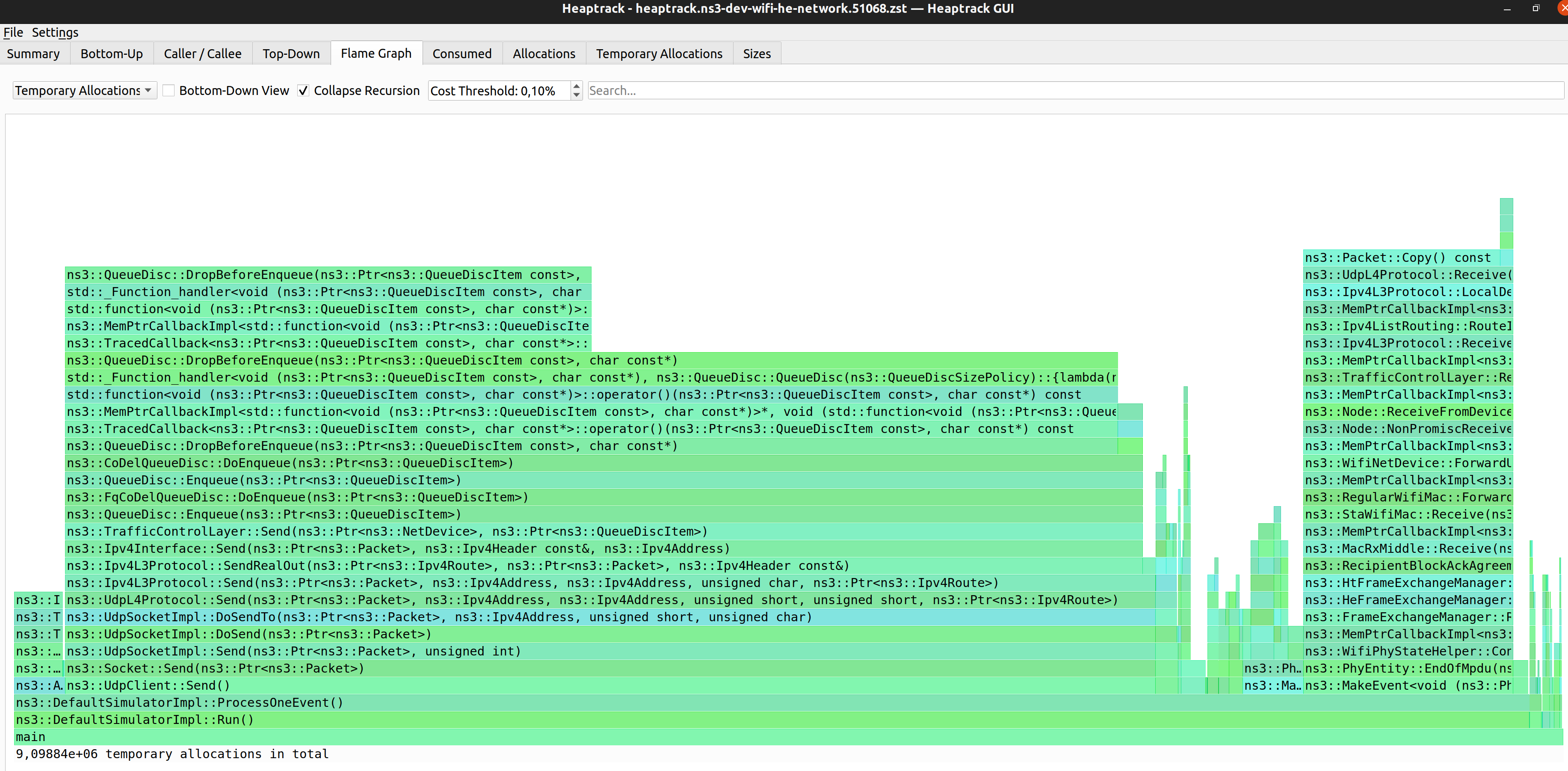
Heaptrack was used in merge request MR830 to track and reduce the number of allocations
in the wifi-he-network example mentioned above. About 29 million unnecessary allocations
were removed, which translates to a 20% reduction. This resulted in a 1.07x speedup of the
test suite with Valgrind (./test.py -d -g) and 1.02x speedup without it.
4.9.1.4. Memray
Memray is an utility made by Bloomberg to trace memory allocations of Python programs, including native code called by them. Along with stack traces, developers can trace down possible memory leaks and unnecessary allocations.
Note: Memray is ineffective for profiling the ns-3 python bindings since Cppyy hides away the calls to the ns-3 module libraries. However, it is still useful for python scripts in general, for example ones used to parse and consolidate simulation results.
The ns3 script includes a run option to launch Python programs with Memray.
Memray can produce different types of reports, such as a flamegraph in HTML, or
text reports (summary and stats).
~/ns-3-dev/$ ./ns3 run sample-rng-plot.py --memray
Writing profile results into memray.output
Memray WARNING: Correcting symbol for aligned_alloc from 0x7fd97023c890 to 0x7fd97102fce0
[memray] Successfully generated profile results.
You can now generate reports from the stored allocation records.
Some example commands to generate reports:
/usr/bin/python3 -m memray flamegraph memray.output
~/ns-3-dev$ /usr/bin/python3 -m memray stats memray.output
Total allocations:
5364235
Total memory allocated:
10.748GB
Histogram of allocation size:
min: 0.000B
----------------------------------------------
< 8.000B : 264149 |||
< 78.000B : 2051906 |||||||||||||||||||||||
< 699.000B : 2270941 |||||||||||||||||||||||||
< 6.064KB : 608993 |||||||
< 53.836KB : 165307 ||
< 477.912KB: 2220 |
< 4.143MB : 511 |
< 36.779MB : 188 |
< 326.492MB: 19 |
<=2.830GB : 1 |
----------------------------------------------
max: 2.830GB
Allocator type distribution:
MALLOC: 4647765
CALLOC: 435525
REALLOC: 277736
POSIX_MEMALIGN: 2686
MMAP: 523
Top 5 largest allocating locations (by size):
- include:/usr/local/lib/python3.10/dist-packages/cppyy/__init__.py:243 -> 8.814GB
- <stack trace unavailable> -> 746.999MB
- show:~/.local/lib/python3.10/site-packages/matplotlib/backends/backend_gtk4.py:340 -> 263.338MB
- load_library:/usr/local/lib/python3.10/dist-packages/cppyy/__init__.py:235 -> 245.684MB
- __init__:/usr/lib/python3.10/ctypes/__init__.py:374 -> 225.797MB
Top 5 largest allocating locations (by number of allocations):
- include:/usr/local/lib/python3.10/dist-packages/cppyy/__init__.py:243 -> 2246145
- show:~/.local/lib/python3.10/site-packages/matplotlib/backends/backend_gtk4.py:340 -> 1264614
- <stack trace unavailable> -> 1098543
- __init__:~/.local/lib/python3.10/site-packages/matplotlib/backends/backend_gtk4.py:61 -> 89466
- run:/usr/lib/python3/dist-packages/gi/overrides/Gio.py:42 -> 79582
4.9.2. Performance Profilers
Performance profilers are programs that collect runtime information and help to identify performance bottlenecks. In some cases, they can point out hotspots and suggest solutions.
There are many tools to profile your program, including:
profilers from CPU manufacturers, such as AMD uProf and Intel VTune
profilers from the operating systems, such as Linux’s Perf and Windows Performance Toolkit
instrumented compilation and auxiliary tools provided by compilers, such as Gprof
An overview on how to use Perf with Hotspot, AMD uProf and Intel VTune is provided in the following sections.
4.9.2.1. Profiling and optimization
While profilers will help point out interest hotspots, they won’t help fixing the issues. At least for now…
After profiling, optimization should be done following the Pareto principle.
Focus first on least amount of work that can provide most benefits.
Let us see an example, based on lte-frequency-reuse. In the example
below you will see a flamegraph generated from the CPU-cycles metrics
collected by perf for this LTE example.

The vertical axis contain stacked bars. Every bar corresponds to a function.
The stack itself represents the call stack (when a function call other,
and other, etc). The width of each bar corresponds to the time it takes to
execute the function itself and the functions it calls (bars on top of it).
This is where we start looking for bottlenecks. Start looking at widest
columns at the top, and move down. As an example, we can select
LteChunkProcessor::End() (highlighted in purple).

If we click on the LteChunkProcessor::End(), we have a closer view of
where it is actually spending time on. We can see many bars related to callback
indirections. Note that each bar is slightly shorter and offset to the right.
This small difference is the overhead of each function call. When everything
is added together, it corresponds to about 35% of total time of
LteChunkProcessor::End(). Yes, callbacks are really expensive,
even in optimized builds. Now, let us take a look at the big gap and big
LteAmc function being called by this callback.

Now that we are closed to the top of the stack, we have a better idea of what is actually happening and can optimize more easily.
For example, notice that about 14% of LteAmc::CreateCqiFeedbacks() is
spent on itself (gap on top of bar). This usually means one of the following:
many conditional operations (if-else, switches), causing instruction cache-misses or pipeline stalls in case of wrong branch prediction
accessing data in erratic patterns, causing data cache-misses
waiting for a value to be computed at a congested CPU unit (e.g. slow division, trigonometric), causing pipeline stalls
a lot of actual work, also known as retired instructions
To check which case it really is, instead of CPU-cycles, one can collect complementary metrics
such as cache-misses, branch-misses, stalled-cycles-frontend, stalled-cycles-backend.
It is easy to spot which one of them is the actual culprit, because its bar will be wider.
After figuring out the issue, you need to look at the code to locate the source of the issue.
Some profilers, such as Intel VTune and AMD uProf can give you the rough location of the
instructions (line of code) causing these misses and stalls.
We also see that 86% of the time is spent elsewhere. In LteMiErrorModel, and some vector related calls.
One of these vector calls is push_back, which takes incredible 30% of the time.
Now let us look at the code to see where we can improve it.
std::vector<int>
LteAmc::CreateCqiFeedbacks(const SpectrumValue& sinr, uint8_t rbgSize)
{
NS_LOG_FUNCTION(this);
std::vector<int> cqi;
if (m_amcModel == MiErrorModel)
{
NS_LOG_DEBUG(this << " AMC-VIENNA RBG size " << (uint16_t)rbgSize);
NS_ASSERT_MSG(rbgSize > 0, " LteAmc-Vienna: RBG size must be greater than 0");
std::vector<int> rbgMap;
int rbId = 0;
for (auto it = sinr.ConstValuesBegin(); it != sinr.ConstValuesEnd(); it++)
{
/// WE CAN CUT 30% OF TIME BY AVOIDING THESE REALLOCATIONS WITH rbgMap.resize(rbgSize) AT BEGINNING
/// THEN USING std::iota(rbgMap.begin(), rbgMap.end(),rbId+1-rbgSize) INSIDE THE NEXT IF
rbgMap.push_back(rbId++);
if ((rbId % rbgSize == 0) || ((it + 1) == sinr.ConstValuesEnd()))
{
uint8_t mcs = 0;
TbStats_t tbStats;
while (mcs <= 28)
{
HarqProcessInfoList_t harqInfoList;
tbStats = LteMiErrorModel::GetTbDecodificationStats(
sinr,
rbgMap,
(uint16_t)GetDlTbSizeFromMcs(mcs, rbgSize) / 8, /// DIVISIONS ARE EXPENSIVE. OPTIMIZER WILL
/// REPLACE THIS TRIVIAL CASE WITH >> 3,
/// BUT THIS ISN'T ALWAYS THE CASE.
/// IF THE DIVISION IS BY A LOOP INVARIANT,
/// THEN COMPUTE ITS INVERSE OUTSIDE
/// THE LOOP TO REPLACE THE DIVISION WITH
/// A MULTIPLICATION.
mcs,
harqInfoList);
if (tbStats.tbler > 0.1)
{
break;
}
mcs++;
}
if (mcs > 0)
{
mcs--;
}
NS_LOG_DEBUG(this << "\t RBG " << rbId << " MCS " << (uint16_t)mcs << " TBLER "
<< tbStats.tbler);
int rbgCqi = 0;
if ((tbStats.tbler > 0.1) && (mcs == 0))
{
rbgCqi = 0; // any MCS can guarantee the 10 % of BER
}
else if (mcs == 28)
{
rbgCqi = 15; // all MCSs can guarantee the 10 % of BER
}
else
{
double s = SpectralEfficiencyForMcs[mcs];
rbgCqi = 0;
while ((rbgCqi < 15) && (SpectralEfficiencyForCqi[rbgCqi + 1] < s))
{
++rbgCqi;
}
}
NS_LOG_DEBUG(this << "\t MCS " << (uint16_t)mcs << "-> CQI " << rbgCqi);
// fill the cqi vector (per RB basis)
/// WE CAN CUT 30% OF TIME BY AVOIDING THESE REALLOCATIONS WITH cqi.resize(cqi.size()+rbgSize)
/// THEN std::fill(cqi.rbegin(), cqi.rbegin()+rbgSize, rbgCqi)
for (uint8_t j = 0; j < rbgSize; j++)
{
cqi.push_back(rbgCqi);
}
rbgMap.clear();
}
}
}
return cqi;
}
Try to explore by yourself with the interactive flamegraph below (only available for html-based documentation).
Note: interactive flamegraph SVGs were generated with perf.data output exported by Linux Perf, then transformed to text and finally rendered as SVG.
git clone https://github.com/brendangregg/FlameGraph
./FlameGraph/stackcollapse-perf.pl perf.data > perf.folded
./FlameGraph/flamegraph.pl perf.folded --width=800 > perf.svg
4.9.2.2. Linux Perf and Hotspot GUI
Perf is the kernel tool to measure performance of the Linux kernel, drivers and user-space applications.
Perf tracks some performance events, being some of the most important for performance:
cycles
Clocks (time) spent running.
cache-misses
When either data or instructions were not in the L1/L2 caches, requiring a L3 or memory access.
branch-misses
How many branch instructions were mispredicted. Mispredictions causes the CPU to stall and clean the pipeline, slowing down the program.
stalled-cycles-frontend
Cycles wasted by the processor waiting for the next instruction, usually due to instruction cache miss or mispredictions. Starves the CPU pipeline of instructions and slows down the program.
stalled-cycles-backend
Cycles wasted waiting for pipeline resources to finish their work. Usually waiting for memory read/write, or executing long-latency instructions.
Just like with heaptrack, perf can be executed using the ns3 wrapper
command template. In the following command we output perf data from wifi-he-network
to the perf.data output file.
~/ns-3-dev$ ./ns3 run "wifi-he-network --simulationTime=0.3 --frequency=5 --useRts=1 --minExpectedThroughput=6 --maxExpectedThroughput=745" --command-template "perf record -o ./perf.data --call-graph dwarf --event cycles,cache-misses,branch-misses --sample-cpu %s" --no-build
For ease of use, ns3 also provides the --perf run option, that
include the recommended settings.
~/ns-3-dev$ ./ns3 run "wifi-he-network --simulationTime=0.3 --frequency=5 --useRts=1 --minExpectedThroughput=6 --maxExpectedThroughput=745" --perf --no-build
When running for the first time, you may receive the following error:
~/ns-3-dev$ ./ns3 run "wifi-he-network --simulationTime=0.3 --frequency=5 --useRts=1 --minExpectedThroughput=6 --maxExpectedThroughput=745" --perf --no-build
Error:
Access to performance monitoring and observability operations is limited.
Consider adjusting /proc/sys/kernel/perf_event_paranoid setting to open
access to performance monitoring and observability operations for processes
without CAP_PERFMON, CAP_SYS_PTRACE or CAP_SYS_ADMIN Linux capability.
More information can be found at 'Perf events and tool security' document:
https://www.kernel.org/doc/html/latest/admin-guide/perf-security.html
perf_event_paranoid setting is 1:
-1: Allow use of (almost) all events by all users
Ignore mlock limit after perf_event_mlock_kb without CAP_IPC_LOCK
>= 0: Disallow raw and ftrace function tracepoint access
>= 1: Disallow CPU event access
>= 2: Disallow kernel profiling
To make the adjusted perf_event_paranoid setting permanent preserve it
in /etc/sysctl.conf (e.g. kernel.perf_event_paranoid = <setting>)
Command 'build/examples/wireless/ns3-dev-wifi-he-network-default record --call-graph dwarf -a -e cache-misses,branch-misses,cpu-cycles,instructions,context-switches build/examples/wireless/ns3-dev-wifi-he-network-default -n=100' returned non-zero exit status 255.
This error is related to lacking permissions to access performance events from the kernel and CPU.
As said in the error, permissions can be granted for the current session
by changing the perf_event_paranoid setting with echo 0 > /proc/sys/kernel/perf_event_paranoid.
This change can be made permanent by changing the setting in /etc/sysctl.conf, but
this is not recommended. Administrative permissions (sudo su) are required in both cases.
After the program finishes, it will print recording statistics.
MCS value Channel width GI Throughput
0 20 MHz 3200 ns 6.01067 Mbit/s
0 20 MHz 1600 ns 5.936 Mbit/s
...
11 160 MHz 1600 ns 493.397 Mbit/s
11 160 MHz 800 ns 534.016 Mbit/s
[ perf record: Woken up 9529 times to write data ]
Warning:
Processed 517638 events and lost 94 chunks!
Check IO/CPU overload!
Warning:
1 out of order events recorded.
[ perf record: Captured and wrote 2898,307 MB perf.data (436509 samples) ]
Results saved in perf.data can be reviewed with the perf report command.
Hotspot is a GUI for Perf, that makes performance profiling more
enjoyable and productive. It can parse the perf.data and show in
a more friendly way.
To record the same perf.data from Hotspot directly, fill the fields
for working directory, path to the executable, arguments, perf
events to track and output directory for the perf.data.
Then run to start recording.
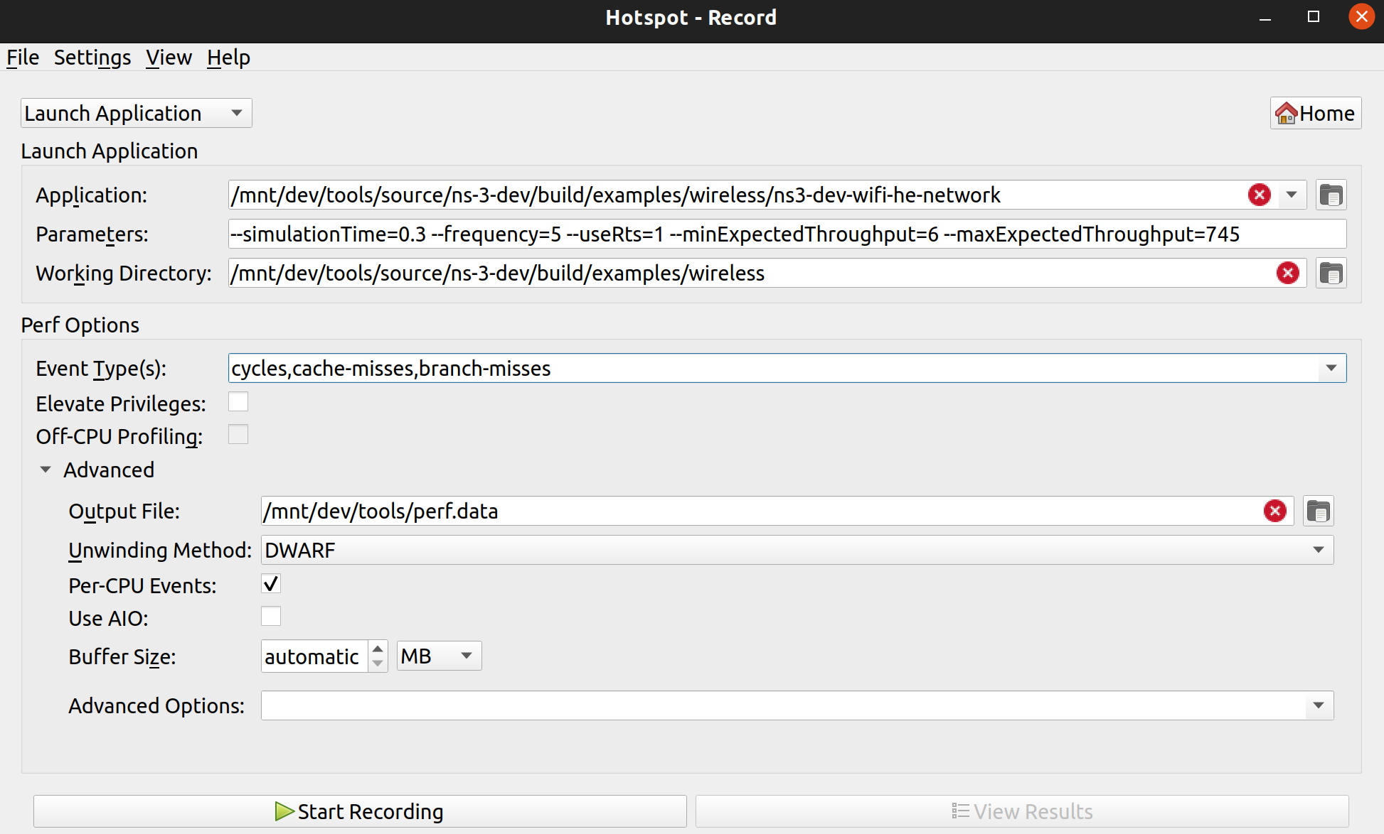
The cycles per function for this program is shown in the following image.
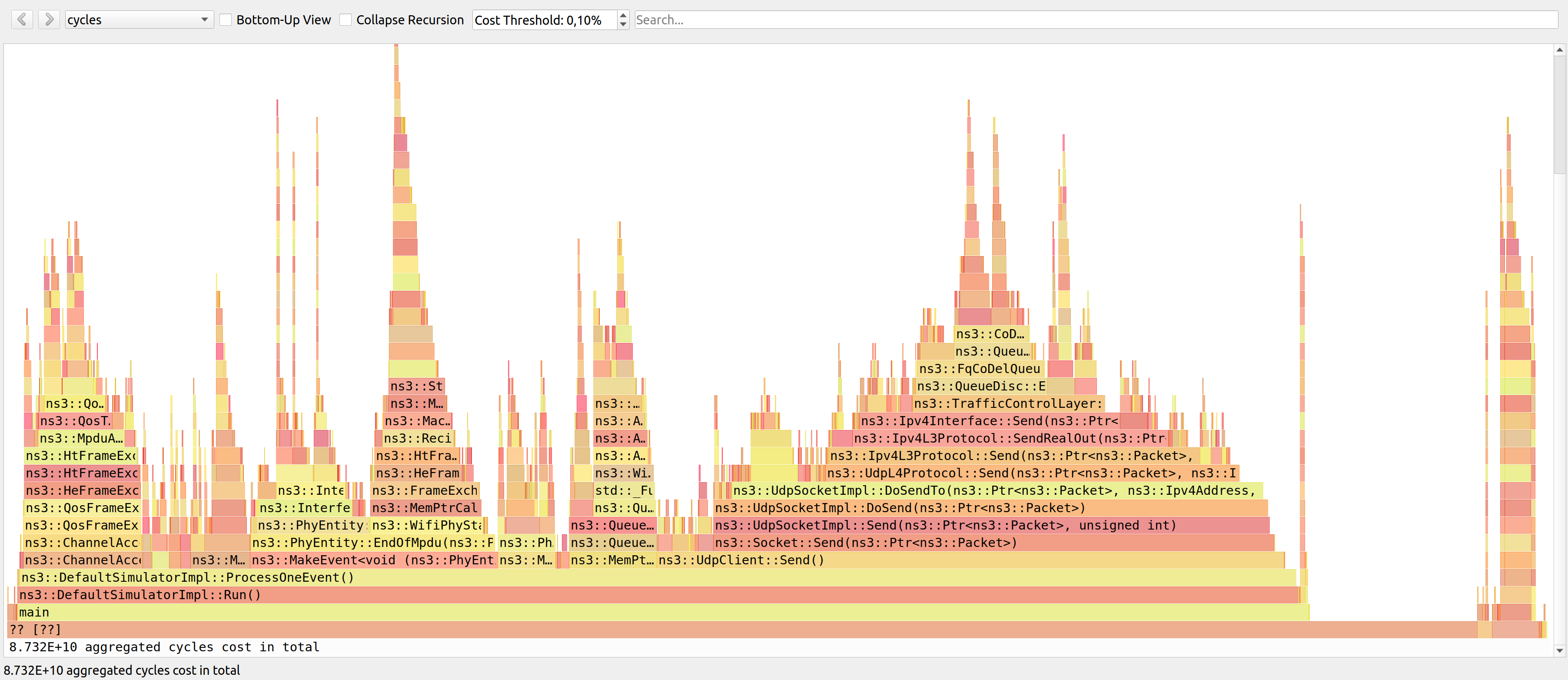
The data is also presented in a tabular format in the bottom-up, top-down and caller/callee tabs (top left of the screen).
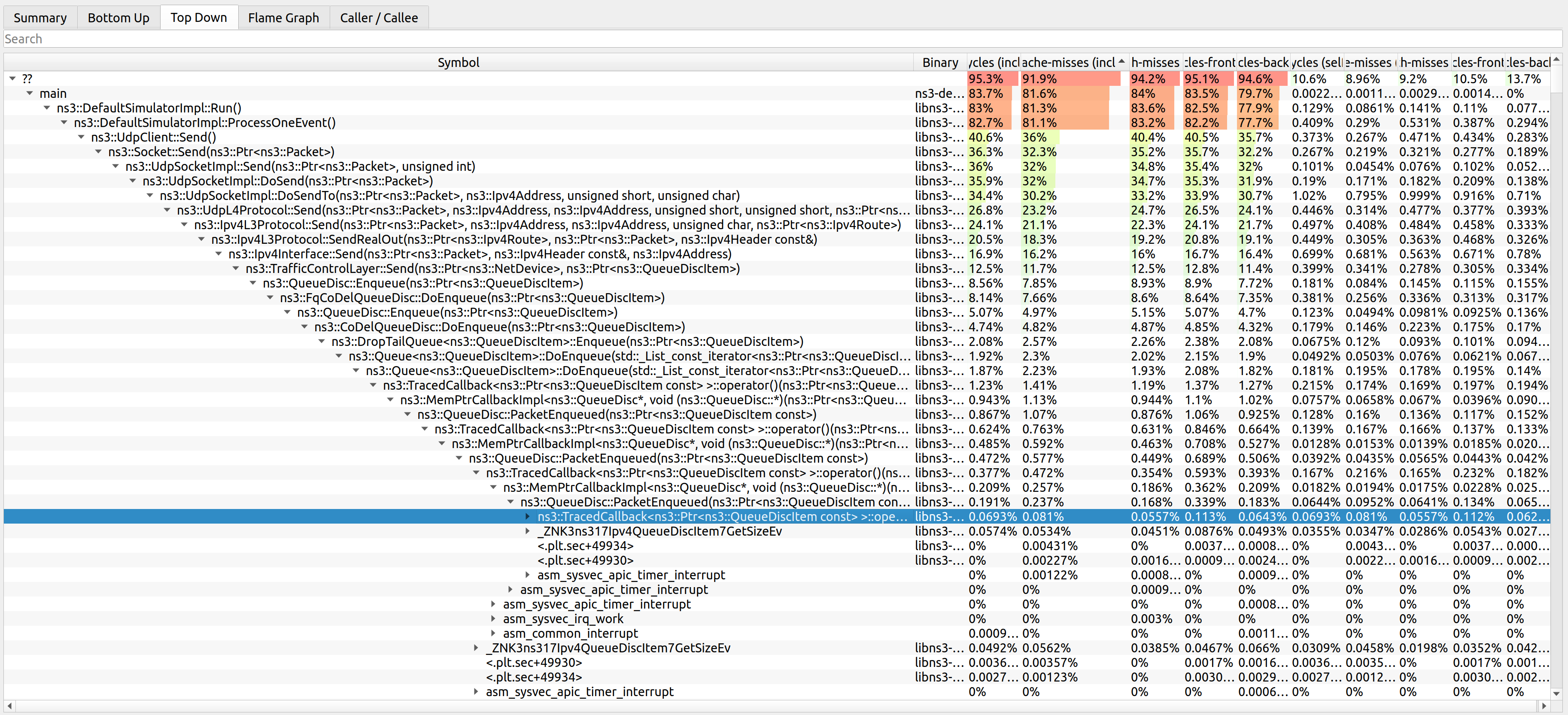
Hotspot was used to identify performance bottlenecks in multiple occasions:
wifi-primary-channelstest suite was extremely slow due to unnecessary RF processing. The adopted solution was to replace the filtering step of the entire channel to just the desired sub-band, and assuming sub-bands are uniformly sized, saving multiplications in the integral used to compute the power of each sub-band. This resulted in a 6x speedup with./ns3 run "test-runner --fullness=TAKES_FOREVER --test-name=wifi-primary-channels". Hotspot was used along with AMD uProf to track this and other bottlenecks in issue 426.WifiMacQueue::TtlExceededdereferenced data out of cache when calling Simulator::Now(). The adopted solution was to move Simulator::Now() out of TtlExceeded and reuse the value and inlining TtlExceeded. This resulted in a ~1.20x speedup with the test suite (./test.py -d). Hotspot was used along with AMD uProf to track this and other bottlenecks in issue 280 and merge request MR681.MpduAggregator and MsduAggregator required an expensive attribute lookup to get the maximum sizes from the RegularWifiMac. Bypassing the attribute lookup reduced cache misses and unnecessary branches. The adopted solution was to move Simulator::Now() out of TtlExceeded and reuse the value and inlining TtlExceeded. This resulted in a ~1.02x speedup with the test suite (
./test.py -d). More details on: merge requests MR681 and MR685.
4.9.2.2.1. Perf on WSL
WSLv1 cannot use perf due to the lack of the linux kernel and its performance counters.
WSLv2 users need to manually build perf to profile their programs, which can be accomplished with the following commands:
sudo apt install git flex bison libdwarf-dev libelf-dev libnuma-dev \
libunwind-dev libnewt-dev libdwarf++0 libelf++0 libdw-dev \
libbfb0-dev systemtap-sdt-dev libssl-dev libperl-dev \
python-dev-is-python3 binutils-dev libiberty-dev libzstd-dev \
libcap-dev libbabeltrace-dev libpfm4-dev libtraceevent-dev pkg-config
git clone https://github.com/microsoft/WSL2-Linux-Kernel --depth 1
cd WSL2-Linux-Kernel/tools/perf
make -j8
sudo cp perf /usr/local/bin
Note that hardware performance counters are only available in Windows 11.
4.9.2.3. AMD uProf
AMD uProf works much like Linux Perf and Hotspot GUI, but is available in more platforms (Linux, Windows and BSD) using AMD processors. Differently from Perf, it provides more performance trackers for finer analysis.
To use it, open uProf then click to profile an application. If you
have already profile an application, you can reuse those settings for
another application by clicking in one of the items in the Recently Used
Configurations section.
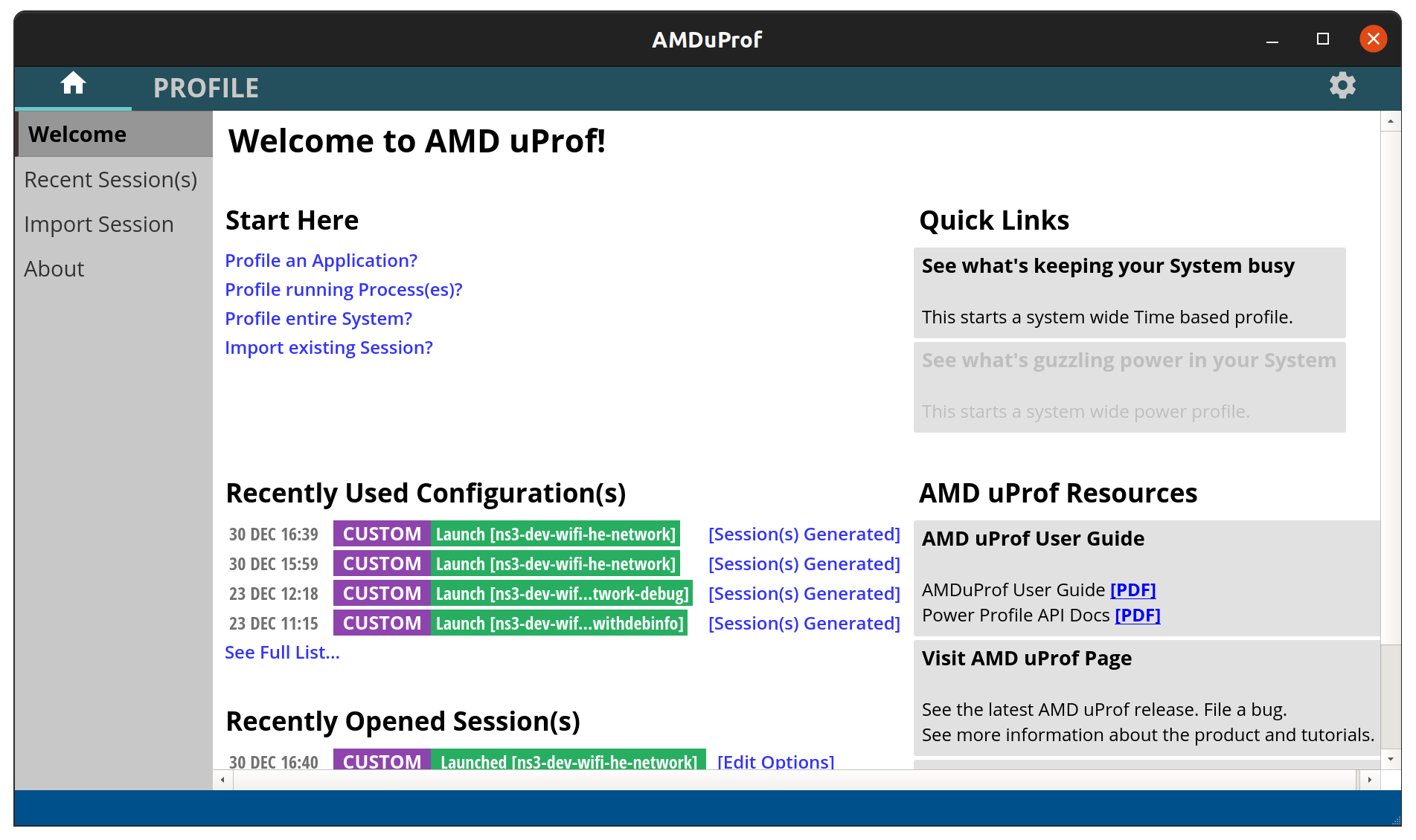
Fill the fields with the application path, the arguments and the working directory.
You may need to add the LD_LIBRARY_PATH environment variable
(or PATH on Windows), pointing it to the library output
directory (e.g. ns-3-dev/build/lib).
Then click next:
Now select custom events and pick the events you want.
- The recommended ones for performance profiling are:
CYCLES_NOT_IN_HALT
Clocks (time) spent running.
RETIRED_INST
How many instructions were completed.
These do not count mispredictions, stalls, etc.
Instructions per clock (IPC) = RETIRED_INST / CYCLES_NOT_IN_HALT
RETIRED_BR_INST_MISP
How many branch instructions were mispredicted.
Mispredictions causes the CPU to stall and clean the pipeline, slowing down the program.
L2_CACHE_MISS.FROM_L1_IC_MISS
L2 cache misses caused by instruction L1 cache misses.
Results in L3/memory accesses due to missing instructions in L1/L2.
L2_CACHE_MISS.FROM_L1_DC_MISS
L2 cache misses caused by data L1 cache misses.
Results in L3/memory accesses due to missing instructions in L1/L2
MISALIGNED_LOADS
Loads not aligned with processor words.
Might result in additional cache and memory accesses.
Now click in advanced options to enable collection of the call stack.
Then click Start Profile and wait for the program to end.
After it finishes you will be greeted with a hotspot summary screen,
but the Analyze tab (top of the screen) has sub-tabs with more
relevant information.
In the following image the metrics are shown per module, including the
C library (libc.so.6) which provides the malloc and free functions.
Values can be shown in terms of samples or percentages for easier reading
and to decide where to optimize.
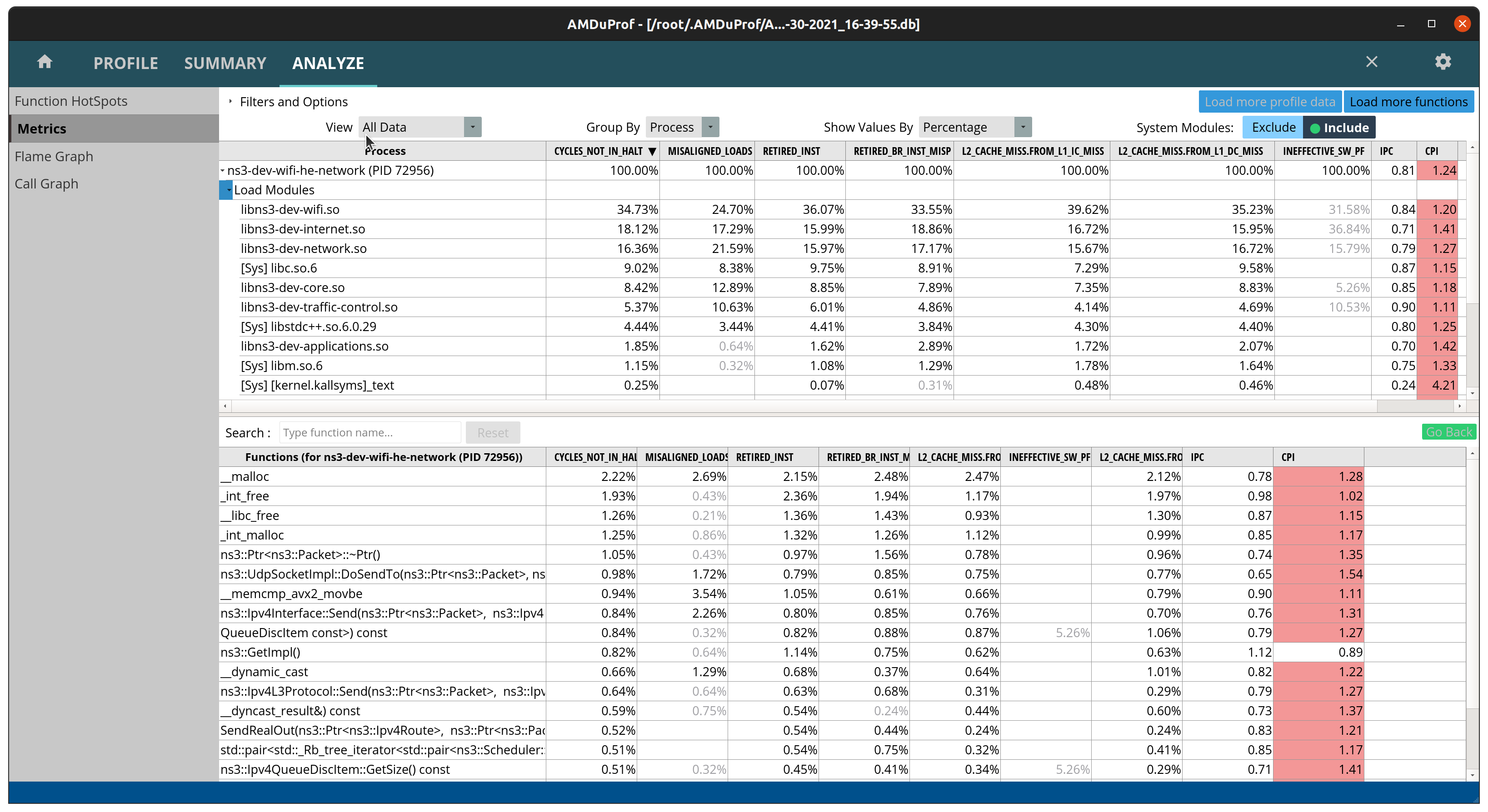
Here are a few cases where AMD uProf was used to identify performance bottlenecks:
WifiMacQueue::TtlExceededdereferenced data out of cache when calling Simulator::Now(). The adopted solution was to move Simulator::Now() out of TtlExceeded and reuse the value and inlining TtlExceeded. This resulted in a ~1.20x speedup with the test suite (./test.py -d). More details on: issue 280 and merge request MR681.wifi-primary-channelstest suite was extremely slow due to unnecessary RF processing. The adopted solution was to replace the filtering step of the entire channel to just the desired sub-band, and assuming sub-bands are uniformly sized, saving multiplications in the integral used to compute the power of each sub-band. This resulted in a 6x speedup with./ns3 run "test-runner --fullness=TAKES_FOREVER --test-name=wifi-primary-channels". More details on: issue 426 and merge request MR677.Continuing the work on
wifi-primary-channelstest suite, profiling showed an excessive number of cache misses inInterferenceHelper::GetNextPosition. This function searches for an iterator on a map, which is very fast if the map is small and fits in the cache, which was not the case. After reviewing the code, it was noticed in most cases this call was unnecessary as the iterator was already known. The adopted solution was to reuse the iterator whenever possible. This resulted in a 1.78x speedup on top of the previous 6x with./ns3 run "test-runner --fullness=TAKES_FOREVER --test-name=wifi-primary-channels". More details on: issue 426 and merge requests MR677 and MR680.Position-Independent Code libraries (
-fPIC) have an additional layer of indirection that increases instruction cache misses. The adopted solution was to disable semantic interposition with flag-fno-semantic-interpositionon GCC. This is the default setting on Clang. This results in approximately 1.14x speedup with./test.py -d. More details on: MR777.
Note: all speedups above were measured on the same machine. Results may differ based on clock speeds, cache sizes, number of cores, memory bandwidth and latency, storage throughput and latency.
4.9.2.4. Intel VTune
Intel VTune works much like Linux Perf and Hotspot GUI, but is available in more platforms (Linux, Windows and Mac) using Intel processors. Differently from Perf, it provides more performance trackers for finer analysis.
When you open the program, you will be greeted by the landing page
shown in the following image. To start a new profiling project, click
in the Configure Analysis button. If you already have a project,
right-click the entry and click to configure analysis to reuse the
settings.
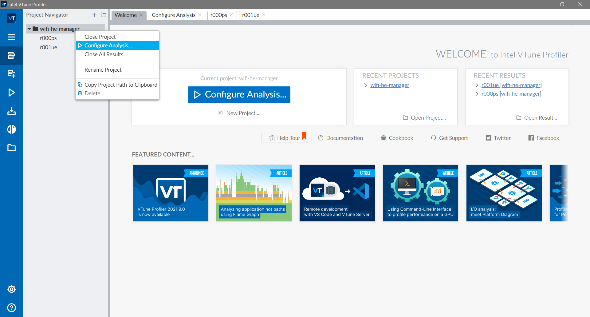
A configuration page will open, where you can fill the fields with the path to the program, arguments, and set working directory and environment variables.
Note: in this example on Windows using MinGW,
we need to define the PATH environment variable with the paths
to both ~/ns-3-dev/build/lib and the MinGW binaries folder
(~/msys64/mingw64/bin), which contains essential libraries.
On Linux-like systems you will need to define the
LD_LIBRARY_PATH environment variable instead of PATH.
Clicking on the Performance Snapshot shows the different profiling
options.
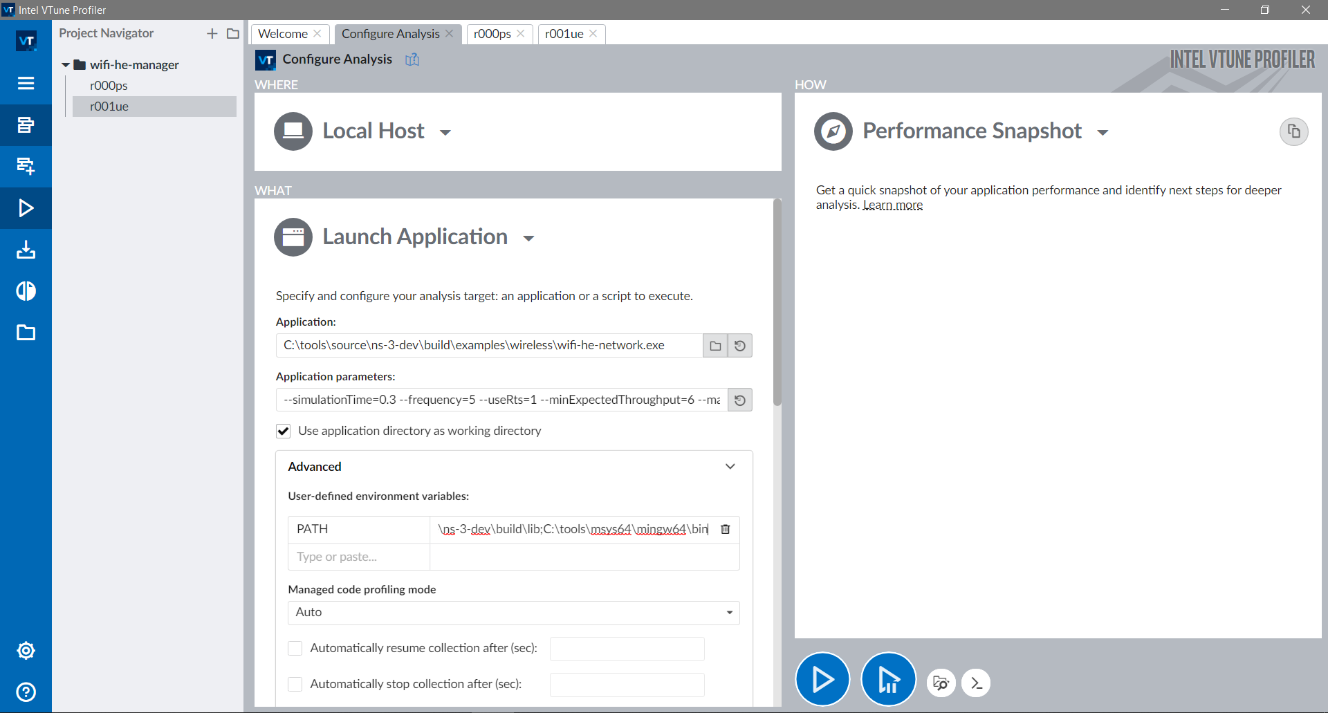
If executed as is, a quicker profiling will be executed to determine what areas should be profiled with more details. For the specific example, it is indicated that there are microarchitectural bottlenecks and low parallelism (not a surprise since ns-3 is single-threaded).
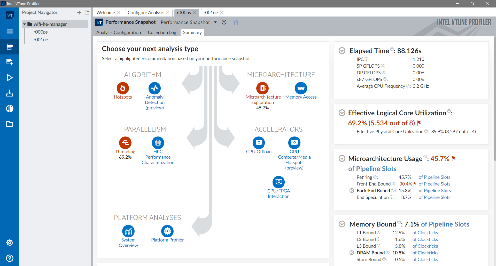
If the microarchitecture exploration option is selected, cycles,
branch mispredictions, cache misses and other metrics will be collected.
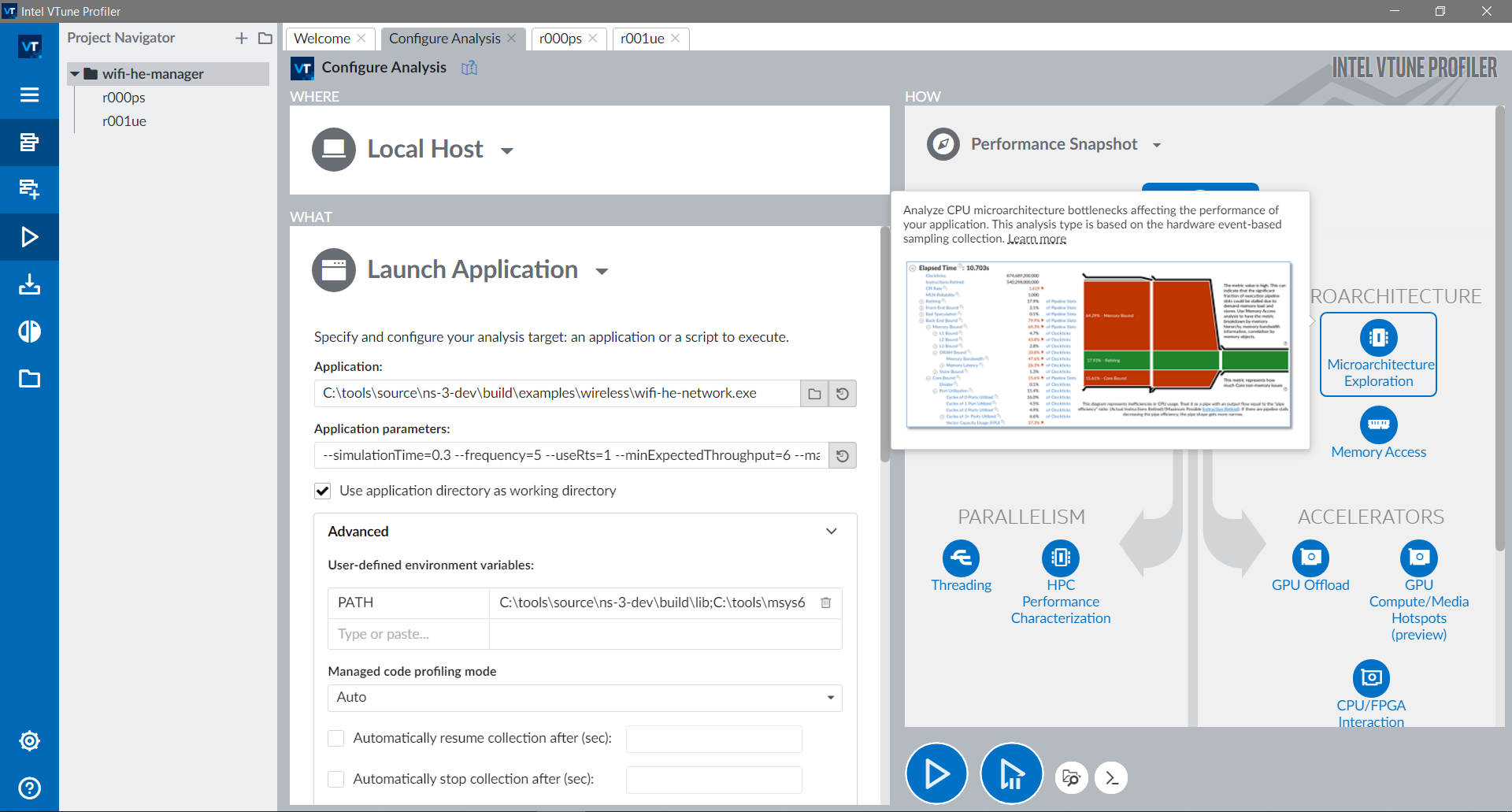
After executing the microarchitecture exploration, a summary will
be shown. Hovering the mouse over the red flags will explain what
each sentence means and how it impacts performance.
Clicking in the Bottom-up tab shows all the information per module.
A plethora of stats such as CPU time, instructions retired,
retiring percentage (how many of the dispatched instructions
were executed until the end, usually lower than 100% because of branch
mispredictions), bad speculation, cache misses, unused load ports,
and more.
The stats for the wifi module are shown below. The retiring metric indicates about 40% of dispatched instructions are executed. The diagram on the right shows the bottleneck is in the front-end of the pipeline (red), due to high instruction cache misses, translation lookaside buffer (TLB) overhead and unknown branches (most likely callbacks).
The stats for the core module are shown below. More specifically for the ns3::Object::DoGetObject function. Metrics indicates about 63% of bad speculations. The diagram on the right shows that there are bottlenecks both in the front-end and due to bad speculation (red).
4.9.3. System calls profilers
System call profilers collect information on which system calls were made by a program, how long they took to be fulfilled and how many of them resulted in errors.
There are many system call profilers, including dtrace, strace and procmon.
An overview on how to use strace is provided in the following section.
4.9.3.1. Strace
The strace is a system calls (syscalls) profiler for Linux. It can filter specific syscalls, or gather stats during the execution.
To collect statistics, use strace -c:
~ns-3-dev/$ ./ns3 run "wifi-he-network --simulationTime=0.3 --frequency=5 --useRts=1 --minExpectedThroughput=6 --maxExpectedThroughput=745" --command-template "strace -c %s" --no-build
MCS value Channel width GI Throughput
0 20 MHz 3200 ns 5.91733 Mbit/s
...
11 160 MHz 800 ns 524.459 Mbit/s
% time seconds usecs/call calls errors syscall
------ ----------- ----------- --------- --------- ----------------
37.62 0.004332 13 326 233 openat
35.46 0.004083 9 415 mmap
...
------ ----------- ----------- --------- --------- ----------------
100.00 0.011515 8 1378 251 total
In the example above, the syscalls are listed in the right, after the time spent on each syscall, number of calls and errors.
The errors can be caused due to multiple reasons and may not
be a problem. To check if they were problems, strace can log the
syscalls with strace -o calls.log:
~ns-3-dev/$ ./ns3 run "wifi-he-network --simulationTime=0.3 --frequency=5 --useRts=1 --minExpectedThroughput=6 --maxExpectedThroughput=745" --command-template "strace -o calls.log %s" --no-build
MCS value Channel width GI Throughput
0 20 MHz 3200 ns 5.91733 Mbit/s
...
11 160 MHz 800 ns 524.459 Mbit/s
Looking at the calls.log file, we can see different sections. In the
following section, the example is executed (execve), architecture is checked (arch_prctl),
memory is mapped for execution (mmap) and LD_PRELOAD use is checked.
execve("~/ns-3-dev/build/examples/wireless/ns3-dev-wifi-he-network", ["~/ns-3-dev/b"..., "--simulationTime=0.3", "--frequency=5", "--useRts=1", "--minExpectedThroughput=6", "--maxExpectedThroughput=745"], 0x7fffb0f91ad8 /* 3 vars */) = 0
brk(NULL) = 0x563141b37000
arch_prctl(0x3001 /* ARCH_??? */, 0x7ffff8d63a50) = -1 EINVAL (Invalid argument)
mmap(NULL, 8192, PROT_READ|PROT_WRITE, MAP_PRIVATE|MAP_ANONYMOUS, -1, 0) = 0x7f103c2e9000
access("/etc/ld.so.preload", R_OK) = -1 ENOENT (No such file or directory)
Then the program searches for the wifi module library and fails multiple times (the errors seen in the table above).
openat(AT_FDCWD, "~/ns-3-dev/build/lib/glibc-hwcaps/x86-64-v3/libns3-dev-wifi.so", O_RDONLY|O_CLOEXEC) = -1 ENOENT (No such file or directory)
newfstatat(AT_FDCWD, "~/ns-3-dev/build/lib/glibc-hwcaps/x86-64-v3", 0x7ffff8d62c80, 0) = -1 ENOENT (No such file or directory)
...
openat(AT_FDCWD, "~/ns-3-dev/build/lib/x86_64/libns3-dev-wifi.so", O_RDONLY|O_CLOEXEC) = -1 ENOENT (No such file or directory)
newfstatat(AT_FDCWD, "~/ns-3-dev/build/lib/x86_64", 0x7ffff8d62c80, 0) = -1 ENOENT (No such file or directory)
The library is finally found and its header is read:
openat(AT_FDCWD, "~/ns-3-dev/build/lib/libns3-dev-wifi.so", O_RDONLY|O_CLOEXEC) = 3
read(3, "\177ELF\2\1\1\3\0\0\0\0\0\0\0\0\3\0>\0\1\0\0\0py\30\0\0\0\0\0"..., 832) = 832
Then other modules that wifi depends on are loaded, then execution of the program continues to the main function of the simulation.
Strace was used to track down issues found while running the lena-radio-link-failure example.
Its strace -c table was the following:
% time seconds usecs/call calls errors syscall
------ ----------- ----------- --------- --------- ----------------
31,51 0,246243 2 103480 942 openat
30,23 0,236284 2 102360 write
19,90 0,155493 1 102538 close
16,65 0,130132 1 102426 lseek
1,05 0,008186 18 437 mmap
0,21 0,001671 16 99 newfstatat
0,20 0,001595 11 134 mprotect
0,18 0,001391 14 98 read
...
------ ----------- ----------- --------- --------- ----------------
100,00 0,781554 1 411681 951 total
Notice the number of openat, write, close and lseek calls
are much more frequent than the other calls. These mean
lena-radio-link-failure is opening, then seeking, then writing,
then closing at least one file handler.
Using strace, we can easily find the most frequently used file handlers.
~ns-3-dev/$./ns3 run "lena-radio-link-failure --numberOfEnbs=2 --useIdealRrc=0 --interSiteDistance=700 --simTime=17" --command-template="strace %s"
...
openat(AT_FDCWD, "DlTxPhyStats.txt", O_WRONLY|O_CREAT|O_APPEND, 0666) = 3
lseek(3, 0, SEEK_END) = 9252
write(3, "635\t1\t1\t1\t0\t20\t1191\t0\t1\t0\n", 26) = 26
close(3) = 0
openat(AT_FDCWD, "DlMacStats.txt", O_WRONLY|O_CREAT|O_APPEND, 0666) = 3
lseek(3, 0, SEEK_END) = 11100
write(3, "0.635\t1\t1\t64\t6\t1\t20\t1191\t0\t0\t0\n", 31) = 31
close(3) = 0
openat(AT_FDCWD, "UlMacStats.txt", O_WRONLY|O_CREAT|O_APPEND, 0666) = 3
lseek(3, 0, SEEK_END) = 8375
write(3, "0.635\t1\t1\t64\t6\t1\t0\t85\t0\n", 24) = 24
close(3) = 0
openat(AT_FDCWD, "DlRsrpSinrStats.txt", O_WRONLY|O_CREAT|O_APPEND, 0666) = 3
lseek(3, 0, SEEK_END) = 16058
write(3, "0.635214\t1\t1\t1\t6.88272e-15\t22.99"..., 37) = 37
close(3) = 0
openat(AT_FDCWD, "UlTxPhyStats.txt", O_WRONLY|O_CREAT|O_APPEND, 0666) = 3
...
With the name of the files, we can look at the code that manipulates them.
The issue above was found in MR777, were performance for some LTE examples
regressed for no apparent reason. The flame graph below, produced by AMD uProf,
contains four large columns/”flames” in red, which
correspond to the write, openat, close and lseek syscalls.
Upon closer inspection, these syscalls take a long time to complete due to the underlying filesystem of the machine running the example (NTFS mount using the ntfs-3g FUSE filesystem). In other words, the bottleneck only exists when running the example in slow file systems (e.g. FUSE and network file systems).
The merge request MR814 addressed the issue by keeping the files open throughout the simulation. That alone resulted in a 1.75x speedup.
4.9.4. Compilation Profilers
Compilation profilers can help identifying which steps of the compilation are slowing it down. These profilers are built into the compilers themselves, only requiring third-party tools to consolidate the results.
The GCC feature is mentioned and exemplified, but is not the recommended compilation profiling method. For that, Clang is recommended.
4.9.4.1. GCC
GCC has a special flag -ftime-report, which makes it print a table
with time spent per compilation phase for each compiled file. The printed
output for a file is shown below. The line of --- was inserted for clarity.
Time variable usr sys wall GGC
phase setup : 0.00 ( 0%) 0.00 ( 0%) 0.01 ( 1%) 1478 kB ( 2%)
phase parsing : 0.31 ( 46%) 0.17 ( 85%) 0.48 ( 55%) 55432 kB ( 71%)
phase lang. deferred : 0.03 ( 4%) 0.00 ( 0%) 0.03 ( 3%) 4287 kB ( 5%)
phase opt and generate : 0.32 ( 48%) 0.03 ( 15%) 0.35 ( 40%) 16635 kB ( 21%)
phase last asm : 0.01 ( 1%) 0.00 ( 0%) 0.01 ( 1%) 769 kB ( 1%)
------------------------------------------------------------------------------------
|name lookup : 0.05 ( 7%) 0.02 ( 10%) 0.04 ( 5%) 2468 kB ( 3%)
|overload resolution : 0.05 ( 7%) 0.00 ( 0%) 0.05 ( 6%) 4217 kB ( 5%)
dump files : 0.00 ( 0%) 0.00 ( 0%) 0.01 ( 1%) 0 kB ( 0%)
callgraph construction : 0.01 ( 1%) 0.00 ( 0%) 0.01 ( 1%) 2170 kB ( 3%)
...
preprocessing : 0.05 ( 7%) 0.06 ( 30%) 0.10 ( 11%) 1751 kB ( 2%)
parser (global) : 0.06 ( 9%) 0.03 ( 15%) 0.07 ( 8%) 16303 kB ( 21%)
parser struct body : 0.06 ( 9%) 0.04 ( 20%) 0.08 ( 9%) 12525 kB ( 16%)
parser enumerator list : 0.01 ( 1%) 0.00 ( 0%) 0.00 ( 0%) 112 kB ( 0%)
parser function body : 0.02 ( 3%) 0.02 ( 10%) 0.02 ( 2%) 3039 kB ( 4%)
parser inl. func. body : 0.03 ( 4%) 0.00 ( 0%) 0.01 ( 1%) 2024 kB ( 3%)
parser inl. meth. body : 0.02 ( 3%) 0.01 ( 5%) 0.06 ( 7%) 5792 kB ( 7%)
template instantiation : 0.09 ( 13%) 0.01 ( 5%) 0.13 ( 15%) 12274 kB ( 16%)
...
symout : 0.01 ( 1%) 0.00 ( 0%) 0.02 ( 2%) 8114 kB ( 10%)
...
TOTAL : 0.67 0.20 0.88 78612 kB
In the table above, the first few lines show the five main compilations steps: setup,
parsing, lang. deferred (C++ specific transformations),
opt(imize) and generate (code), last asm (produce binary code).
The lines below the --- line show sub-steps of the five main compilation steps.
For this specific case, parsing global definitions (21%) and structures (16%),
template instantiation (16%) and generating the code in symout (10%).
Aggregating the data into a meaningful output to help focus where to improve is not that easy and it is not a priority for GCC developers.
It is recommended to use the Clang alternative.
4.9.4.2. Clang
Clang can output very similar results with the -ftime-trace flag, but can also aggregate
it in a more meaningful way. With the help of the third-party tool ClangBuildAnalyzer,
we can have really good insights on where to spend time trying to speed up the compilation.
Support for building with -ftime-trace, compiling ClangBuildAnalyzer and producing a
report for the project have been baked into the CMake project of ns-3, and can be enabled
with -DNS3_CLANG_TIMETRACE=ON.
~/ns-3-dev/cmake_cache$ cmake -DNS3_CLANG_TIMETRACE=ON ..
Or via ns3:
~/ns-3-dev$ ./ns3 configure -- -DNS3_CLANG_TIMETRACE=ON
The entire procedure looks like the following:
~/ns-3-dev$ CXX="clang++" ./ns3 configure -d release --enable-examples --enable-tests -- -DNS3_CLANG_TIMETRACE=ON
~/ns-3-dev$ ./ns3 build timeTraceReport
~/ns-3-dev$ cat ClangBuildAnalyzerReport.txt
Analyzing build trace from '~/ns-3-dev/cmake_cache/clangBuildAnalyzerReport.bin'...
**** Time summary:
Compilation (2993 times):
Parsing (frontend): 2476.1 s
Codegen & opts (backend): 1882.9 s
**** Files that took longest to parse (compiler frontend):
8966 ms: src/test/CMakeFiles/libtest.dir/traced/traced-callback-typedef-test-suite.cc.o
6633 ms: src/wifi/examples/CMakeFiles/wifi-bianchi.dir/wifi-bianchi.cc.o
...
**** Files that took longest to codegen (compiler backend):
36430 ms: src/wifi/CMakeFiles/libwifi-test.dir/test/block-ack-test-suite.cc.o
24941 ms: src/wifi/CMakeFiles/libwifi-test.dir/test/wifi-mac-ofdma-test.cc.o
...
**** Templates that took longest to instantiate:
12651 ms: std::unordered_map<int, int> (615 times, avg 20 ms)
10950 ms: std::_Hashtable<int, std::pair<const int, int>, std::allocator<std::... (615 times, avg 17 ms)
10712 ms: std::__detail::__hyperg<long double> (1172 times, avg 9 ms)
...
**** Template sets that took longest to instantiate:
111660 ms: std::list<$> (27141 times, avg 4 ms)
79892 ms: std::_List_base<$> (27140 times, avg 2 ms)
75131 ms: std::map<$> (11752 times, avg 6 ms)
65214 ms: std::allocator<$> (66622 times, avg 0 ms)
...
**** Functions that took longest to compile:
7206 ms: OfdmaAckSequenceTest::CheckResults(ns3::Time, ns3::Time, unsigned ch... (~/ns-3-dev/src/wifi/test/wifi-mac-ofdma-test.cc)
6146 ms: PieQueueDiscTestCase::RunPieTest(ns3::QueueSizeUnit) (~/ns-3-dev/src/traffic-control/test/pie-queue-disc-test-suite.cc)
...
**** Function sets that took longest to compile / optimize:
14801 ms: std::__cxx11::basic_string<$> ns3::CallbackImplBase::GetCppTypeid<$>() (2342 times, avg 6 ms)
12013 ms: ns3::CallbackImpl<$>::DoGetTypeid[abi:cxx11]() (1283 times, avg 9 ms)
10034 ms: ns3::Ptr<$>::~Ptr() (5975 times, avg 1 ms)
8932 ms: ns3::Callback<$>::DoAssign(ns3::Ptr<$>) (591 times, avg 15 ms)
6318 ms: ns3::CallbackImpl<$>::DoGetTypeid() (431 times, avg 14 ms)
...
*** Expensive headers:
293609 ms: ~/ns-3-dev/build/include/ns3/log.h (included 1404 times, avg 209 ms), included via:
cqa-ff-mac-scheduler.cc.o (758 ms)
ipv6-list-routing.cc.o (746 ms)
...
239884 ms: ~/ns-3-dev/build/include/ns3/nstime.h (included 1093 times, avg 219 ms), included via:
lte-enb-rrc.cc.o lte-enb-rrc.h (891 ms)
wifi-acknowledgment.cc.o wifi-acknowledgment.h (877 ms)
...
216218 ms: ~/ns-3-dev/build/include/ns3/object.h (included 1205 times, avg 179 ms), included via:
energy-source-container.cc.o energy-source-container.h energy-source.h (1192 ms)
phased-array-model.cc.o phased-array-model.h (1135 ms)
...
206801 ms: ~/ns-3-dev/build/include/ns3/core-module.h (included 195 times, avg 1060 ms), included via:
sample-show-progress.cc.o (1973 ms)
length-example.cc.o (1848 ms)
...
193116 ms: /usr/bin/../lib/gcc/x86_64-linux-gnu/11/../../../../include/c++/11/bits/basic_string.h (included 1499 times, avg 128 ms), included via:
model-typeid-creator.h attribute-default-iterator.h type-id.h attribute.h string (250 ms)
li-ion-energy-source-helper.h energy-model-helper.h attribute.h string (243 ms)
...
185075 ms: /usr/bin/../lib/gcc/x86_64-linux-gnu/11/../../../../include/c++/11/bits/ios_base.h (included 1495 times, avg 123 ms), included via:
iomanip (403 ms)
mpi-test-fixtures.h iomanip (364 ms)
...
169464 ms: ~/ns-3-dev/build/include/ns3/ptr.h (included 1399 times, avg 121 ms), included via:
lte-test-rlc-um-e2e.cc.o config.h (568 ms)
lte-test-rlc-um-transmitter.cc.o simulator.h event-id.h (560 ms)
...
done in 2.8s.
The output printed out contain a summary of time spent on parsing and on code generation, along
with multiple lists for different tracked categories. From the summary, it is clear that parsing times
are very high when compared to the optimization time (-O3). Skipping the others categories and going straight
to the expensive headers section, we can better understand why parsing times are so high, with some headers
adding as much as 5 minutes of CPU time to the parsing time.
Precompiled headers (-DNS3_PRECOMPILE_HEADERS=ON) can drastically speed up parsing times,
however, they can increase ccache misses, reducing the time of the first
compilation at the cost of increasing recompilation times.
4.9.4.3. NinjaTracing
If the Ninja generator is being used (./ns3 configure -G Ninja), its build log
can be used to identify targets slowing down the build process. The NinjaTracing
utility is used to convert the log format into a tracing Json file.
The following steps show how it can be used:
~/ns-3-dev$ ./ns3 configure --enable-ninja-tracing
~/ns-3-dev$ ./ns3 build
~/ns-3-dev$ ./ns3 build ninjaTrace
The output ninja_performance_trace.json should be located in the ~/ns-3-dev directory.
You can then visualize the results using the about:tracing panel available in
Chromium-based browser or with a compatible trace viewer such as Perfetto UI.
It can also be used in conjunction with the Clang time-trace feature for more granular information from within the compiler and linker.
~/ns-3-dev$ CXX=clang++ ./ns3 configure --enable-ninja-tracing -- -DNS3_CLANG_TIMETRACE=ON
~/ns-3-dev$ ./ns3 build
~/ns-3-dev$ ./ns3 build ninjaTrace
4.9.5. CMake Profiler
CMake has a built-in tracer that permits tracking hotspots in the CMake files slowing down the project configuration. To use the tracer, call cmake directly from a clean CMake cache directory:
~/ns-3-dev/cmake-cache$ cmake .. --profiling-format=google-trace --profiling-output=../cmake_performance_trace.log
Or using the ns3 wrapper:
~/ns-3-dev$ ./ns3 configure --trace-performance
A cmake_performance_trace.log file will be generated in the ns-3-dev directory.
The tracing results can be visualized using the about:tracing panel available
in Chromium-based browsers or a compatible trace viewer such as Perfetto UI.
After opening the trace file, select the traced process and click on any of the blocks to inspect the different stacks and find hotspots. An auxiliary panel containing the function/macro name, arguments and location can be shown, providing enough information to trace back the location of each specific call.
Just like in performance profilers, visual inspection makes it easier to identify hotspots and focus on trying to optimize what matters most.
The trace below was generated during the discussion of issue #588, while investigating the long configuration times, especially when using HDDs.
The single largest contributor was CMake’s configure_file, used to keeping
up-to-date copies of headers in the output directory.
In MR911, alternatives such as stub headers that include the original header files, keeping them in their respective modules, and symlinking headers to the output directory were used to reduce the configuration overhead.
Note: when testing I/O bottlenecks, you may want to drop filesystem caches, otherwise the cache may hide the issues. In Linux, the caches can be cleared using the following command:
~/ns-3-dev$ sudo sysctl vm.drop_caches=3
4.10. Working with gitlab-ci-local
The ns-3 project repository is currently hosted in GitLab, which includes continuous integration (CI) tools to automate build, tests, packaging and distribution of software. The CI works based on jobs, that are defined in YAML files and run inside containers.
See Working with Docker for more information about containers in general.
The ns-3 GitLab CI files are located in ns-3-dev/utils/tests/.
The main GitLab CI file is gitlab-ci.yml. The different jobs
are used to check if a multitude of compilers and package versions
are compatible with the current ns-3 build, which is why a build is
usually followed by a test run. Other CI jobs build and warn about
missing the documentation.
The GitLab CI jobs are executed based on pipelines containing a sequence of job batches. Jobs within a batch can be executed in parallel. These pipelines can be triggered manually, or scheduled to run automatically per commit and/or based on a time period (ns-3 has daily and weekly pipelines scheduled).
The GitLab CI free tier is very slow, taking a lot of time to identify issues during active merge request development.
Note: the free tier now requires a credit card due to crypto miners abuse.
GitLab-CI-local is a tool that allows an user to use the GitLab CI configuration files locally, allowing for the debugging of CI settings and pipelines without requiring pushes to test repositories or main repositories that fill up the CI job queues with failed jobs due to script errors.
GitLab-CI-local relies on Docker containers to setup the environment to execute the jobs.
Note: Docker is usually setup in root mode, requiring frequent use of administrative permissions/sudo. However, this is highly discouraged. You can configure Docker to run in Docker rootless mode. From this point onwards, we assume Docker is configured in Docker rootless mode.
After installing both Docker and GitLab-CI-local, the ns-3 jobs can be listed using the following command:
~/ns-3-dev$ gitlab-ci-local --file ./utils/tests/gitlab-ci.yml --list
parsing and downloads finished in 226 ms
name description stage when allow_failure needs
weekly-build-ubuntu-18.04-debug build on_success false
...
weekly-build-clang-11-optimized build on_success false
cppyy-22.04 build on_success false
per-commit-compile-debug build on_success false
per-commit-compile-release build on_success false
per-commit-compile-optimized build on_success false
daily-test-debug test on_success false
daily-test-release test on_success false
daily-test-optimized test on_success false
daily-test-optimized-valgrind test on_success false
weekly-test-debug-valgrind test on_success false
weekly-test-release-valgrind test on_success false
weekly-test-optimized-valgrind test on_success false
weekly-test-takes-forever-optimized test on_success false
doxygen documentation on_success false
manual documentation on_success false
tutorial documentation on_success false
models documentation on_success false
To execute the per-commit-compile-release job, or any of the others listed above, use
the following command.
~/ns-3-dev$ gitlab-ci-local --file ./utils/tests/gitlab-ci.yml per-commit-compile-release
WARNING: if you do not specify the job name, all jobs that can be executed in parallel will be executed at the same time. You may run out of disk, memory or both.
Some jobs might require a previous job to complete successfully before getting started. The doxygen job is one of these.
~/ns-3-dev$ gitlab-ci-local --file ./utils/tests/gitlab-ci.yml doxygen
Using fallback git user.name
Using fallback git user.email
parsing and downloads finished in 202 ms
doxygen starting archlinux:latest (documentation)
doxygen pulled archlinux:latest in 64 ms
doxygen > still running...
doxygen > still running...
doxygen copied to container in 20 s
doxygen imported cache 'ccache-' in 3.67 s
~/ns-3-dev/.gitlab-ci-local/artifacts/pybindgen doesn't exist, did you forget --needs
As instructed by the previous command output, you can add the --needs to build required
jobs before proceeding. However, doing so will run all jobs as the doxygen is only supposed
to run after weekly jobs are successfully executed.
Another option is to run the specific job that produces the required artifact. In this case
the pybindgen job.
Note: Pybindgen has been replaced by Cppyy, which does not produce artifacts to be consumed by other jobs. However, the example is kept for reference.
~/ns-3-dev$ gitlab-ci-local --file ./utils/tests/gitlab-ci.yml pybindgen
Using fallback git user.name
Using fallback git user.email
parsing and downloads finished in 202 ms
pybindgen starting archlinux:latest (build)
...
pybindgen $ git diff src > pybindgen_new.patch
pybindgen exported artifacts in 911 ms
pybindgen copied artifacts to cwd in 56 ms
pybindgen finished in 5.77 min
PASS pybindgen
Then run the doxygen job again:
~/ns-3-dev$ gitlab-ci-local --file ./utils/tests/gitlab-ci.yml doxygen
Using fallback git user.name
Using fallback git user.email
parsing and downloads finished in 170 ms
doxygen starting archlinux:latest (documentation)
...
doxygen > 1 files with warnings
doxygen > Doxygen Warnings Summary
doxygen > ----------------------------------------
doxygen > 1 directories
doxygen > 1 files
doxygen > 23 warnings
doxygen > done.
doxygen exported cache ns-3-ccache-storage/ 'ccache-' in 6.86 s
doxygen exported artifacts in 954 ms
doxygen copied artifacts to cwd in 59 ms
doxygen finished in 15 min
PASS doxygen
Artifacts built by the CI jobs will be stored in separate subfolders based on the job name.
~/ns-3-dev/.gitlab-ci-local/artifacts/jobname
Note: some jobs may access the CI_DEFAULT_BRANCH environment variable,
which is set by default to main instead of master. To change that, we need
to create a file ~/.gitlab-ci-local/variables.yml containing the following:
global:
CI_DEFAULT_BRANCH: "master"
In case you are using Docker with root, you need to create this file in
/root/.gitlab-ci-local/variables.yml.
4.11. Working with Docker
The ns-3 project repository is currently hosted in GitLab, which includes continuous integration (CI) tools to automate build, tests, packaging and distribution of software. The CI works based on jobs, that are defined in YAML files, which specify a container the job will run on.
See Working with gitlab-ci-local for how to use containers for running our CI checks locally.
A container is a lightweight virtualization tool that allows one to use user space tools from different OSes on top of the same kernel. This drastically cuts the overhead of alternatives such as full virtualization, where a complete operating system and the hardware it runs on needs to be emulated, or the hardware switched between a host and a guest OS via a hypervisor.
The most common type of containers are applications containers, where Docker is the most popular solution.
Note on pricing: notice that commercial and governmental use of Docker may require a subscription. See Docker pricing for more information. Podman is an open-source drop-in replacement.
Note on security: Docker is installed by default with root privileges. This is a security hazard if you are running untrusted software, especially in shared environments. Docker can be installed in rootless mode for better isolation, however, the alternatives such as Podman and Apptainer (previously Singularity) provide safer default settings. You can read more on Docker security.
4.11.1. Docker containers
Docker popularized containers and made them ubiquitous in continuous integration due to its ease of use. This section will consolidate the basics of how to work with Docker or its compatible alternatives.
Docker workflow typically consists of 10 steps:
4.11.1.1. Install Docker
Docker is usually set up (e.g. via system package managers or their official installers) in root mode, requiring frequent use of administrative permissions/sudo, which is necessary for some services, but not for most. For proper isolation, install Docker in rootless mode, or use one of its compatible alternatives.
4.11.1.2. Write a Dockerfile
A Dockerfile is a file that contains instructions of how to build an image of the container that will host the application / service. These files are composed of one-line commands using special keywords. The most common keywords are:
FROM: used to specify a parent imageCOPY: used to copy files from the external build directory into the containerRUN: run shell commands to install dependencies and set up the serviceENTRYPOINT: program to be started when the container is launched
Here is one example of a Dockerfile that can be used to debug a ns-3
program on Fedora 37:
FROM fedora:37
RUN dnf update --assumeyes && dnf install --assumeyes gcc-c++ cmake ccache ninja-build python gdb
ENTRYPOINT ["bash"]
When Docker is called to build the container image for this Dockerfile, it will
pull the image for fedora:37 from a Docker Registry. Common registries
include docker.io (which hosts images shown in the DockerHub webpage), quay.io,
GitHub, GitLab, or you can have your own self-hosted option.
Note: For security reasons, it is not recommended to run third-party images in production. Dockerfiles are embedded into docker images and can be checked. One example of how this can be done is shown below:
$ docker image ls
REPOSITORY TAG IMAGE ID CREATED SIZE
fedoradebugging 37 d96491e23a80 10 days ago 829 MB
$ docker history fedoradebugging
ID CREATED CREATED BY SIZE COMMENT
0b56b184852b 10 days ago /bin/sh -c #(nop) ENTRYPOINT ["bash"] 0 B
<missing> 10 days ago /bin/sh -c dnf update --assumeyes && dnf i... 648 MB FROM registry.fedoraproject.org/fedora:37
4105b568d464 2 months ago 182 MB Created by Image Factory
We can see different layers (commands) that compose the final docker image.
When compared to the Dockerfile, they show up in reverse order from the latest
to the earliest event.
4.11.1.3. Build a Docker container image
When building toolchain containers to work on projects, we typically don’t want to copy the projects themselves into the container. So we need to pass an empty directory to Docker.
We also need to specify a tag for our image, otherwise it will have a randomly assigned name which we will have to refer to later.
$ mkdir empty-dir
$ docker image ls
REPOSITORY TAG IMAGE ID CREATED SIZE
$ docker build -t fedoradebugging:37 -f Dockerfile ./empty-dir
STEP 1/3: FROM fedora:37
Resolved "fedora" as an alias (/etc/containers/registries.conf.d/shortnames.conf)
Trying to pull registry.fedoraproject.org/fedora:37...
Getting image source signatures
Copying blob 80b613d8f1ff done
Copying config 4105b568d4 done
Writing manifest to image destination
Storing signatures
STEP 2/3: RUN dnf update --assumeyes && dnf install --assumeyes gcc-c++ cmake ccache ninja-build python gdb
Fedora 37 - x86_64 4.0 MB/s | 82 MB 00:20
Fedora 37 openh264 (From Cisco) - x86_64 2.1 kB/s | 2.5 kB 00:01
Fedora Modular 37 - x86_64 1.6 MB/s | 3.8 MB 00:02
Fedora 37 - x86_64 - Updates 5.0 MB/s | 41 MB 00:08
Fedora Modular 37 - x86_64 - Updates 1.3 MB/s | 2.9 MB 00:02
Last metadata expiration check: 0:00:01 ago on Fri Feb 2 13:41:30 2024.
Dependencies resolved.
================================================================================
Package Arch Version Repository Size
================================================================================
Upgrading:
elfutils-default-yama-scope noarch 0.190-2.fc37 updates 12 k
...
(38/56): cmake-3.27.7-1.fc37.x86_64.rpm 1.8 MB/s | 7.8 MB 00:04
(39/56): cpp-12.3.1-1.fc37.x86_64.rpm 1.8 MB/s | 11 MB 00:05
...
Complete!
--> c33f842f2fc
STEP 3/3: ENTRYPOINT ["bash"]
COMMIT fedoradebugging:37
--> 2412e124d12
Successfully tagged localhost/fedoradebugging:37
2412e124d1257914a70fde70289948f7880fdbd1d3b213c206ff691995ecc03e
$ docker image ls
REPOSITORY TAG IMAGE ID CREATED SIZE
localhost/fedoradebugging 37 2412e124d125 About a minute ago 829 MB
registry.fedoraproject.org/fedora 37 4105b568d464 2 months ago 182 MB
Notice that our image got the repository name prepended (localhost).
This is a Podman thing, with the objective people specify the repositories
their images come from, instead of risking pulling an image from different
registries and risk pulling an infected image.
4.11.1.4. Create a container based on the image
Note: For toolchain containers, which is the typical use case
for ns-3 testing, we use the run command instead. It creates
and starts the container in a single command. You can jump directly
to the intended way to use toolchain containers, or continue
reading in case you want to learn a bit more about Docker.
Now that we have our container image, we can create a container based on it. It is like booting a brand-new computer with a freshly installed operating system and commonly used programs.
Docker containers can be created with the following:
$ docker container ls -a
CONTAINER ID IMAGE COMMAND CREATED STATUS PORTS NAMES
$ docker container create --name fedoradeb fedoradebugging:37
8cb9edea0dcfe4a2335dd5b73766a6985275f9ee3e0b6fd5ea5b03eedbd4bbb1
$ docker container ls -a
CONTAINER ID IMAGE COMMAND CREATED STATUS PORTS NAMES
8cb9edea0dcf localhost/fedoradebugging:37 13 seconds ago Created fedoradeb
4.11.1.5. Start the container
Containers can be started with the following commands:
$ docker start fedoradeb
fedoradeb
$ docker container ls -a
CONTAINER ID IMAGE COMMAND CREATED STATUS PORTS NAMES
8cb9edea0dcf localhost/fedoradebugging:37 About a minute ago Exited (0) 13 seconds ago fedoradeb
As it can be seen, our container was started, then executed bash, but it was in a non-interactive session, so it doesn’t wait for the user. The process created by the entrypoint then exited, and the container manager stopped the container.
This is useful for containers running services, like web servers, but not useful at all to use it as a toolchain container. In the next section, we see the preferred way to start a container toolchain.
4.11.1.6. Access the container
For service containers, after starting the container with
start, we can execute commands on the running container
using exec. We are going to use a different container for
demonstration purposes.
$ docker pull nginx:latest
Resolving "nginx" using unqualified-search registries (/etc/containers/registries.conf)
Trying to pull docker.io/library/nginx:latest...
Getting image source signatures
Copying blob 398157bc5c51 done
Copying blob f0bd99a47d4a done
Copying blob f24a6f652778 done
Copying blob c57ee5000d61 done
Copying blob 9f3589a5fc50 done
Copying blob 9b0163235c08 done
Copying blob 1ef1c1a36ec2 done
Copying config b690f5f0a2 done
Writing manifest to image destination
Storing signatures
b690f5f0a2d535cee5e08631aa508fef339c43bb91d5b1f7d77a1a05cea021a8
$ docker container create --name nginx nginx:latest
b6fb5a96bed7552a8164ee20e20cb2dd39ac98f6a7c7c076d0e22b93bc85b988
$ docker container ls -a
CONTAINER ID IMAGE COMMAND CREATED STATUS PORTS NAMES
b6fb5a96bed7 docker.io/library/nginx:latest nginx -g daemon o... 16 seconds ago Created nginx
$ docker start nginx
nginx
$ docker exec nginx whereis nginx
nginx: /usr/sbin/nginx /usr/lib/nginx /etc/nginx /usr/share/nginx
$ docker exec -it nginx bash
root@b6fb5a96bed7:/# echo "Printing a message in the container"
Printing a message in the container
root@b6fb5a96bed7:/# exit
exit
$ docker container stop nginx
nginx
$ docker container ls -a
CONTAINER ID IMAGE COMMAND CREATED STATUS PORTS NAMES
b6fb5a96bed7 docker.io/library/nginx:latest nginx -g daemon o... 5 minutes ago Exited (0) 7 seconds ago nginx
$ docker container rm nginx
b6fb5a96bed7552a8164ee20e20cb2dd39ac98f6a7c7c076d0e22b93bc85b988
$ docker container ls -a
CONTAINER ID IMAGE COMMAND CREATED STATUS PORTS NAMES
$ docker image ls
REPOSITORY TAG IMAGE ID CREATED SIZE
docker.io/library/nginx latest b690f5f0a2d5 3 months ago 191 MB
$ docker image rm nginx:latest
Untagged: docker.io/library/nginx:latest
Deleted: b690f5f0a2d535cee5e08631aa508fef339c43bb91d5b1f7d77a1a05cea021a8
4.11.1.6.1. The intended way to access toolchain containers
Other than start/stop/exec, Docker also has a run option, that builds a
brand-new container from the container image for each time it is executed.
This is the intended way to use toolchain containers.
$ docker run -it fedoradebugging:37
[root@6fa29fa742c5 /]# echo "Printing a message in the container"
Printing a message in the container
[root@6fa29fa742c5 /]# exit
exit
$
Now we need to access files that are not inside the container volume. To do this, we can mount an external volume as a local directory.
$ mkdir -p ./external/ns-3-dev
$ echo "hello" > ./external/ns-3-dev/msg.txt
$ docker run -it -v ./external/ns-3-dev:/internal/ns-3-dev fedoradebugging:37
[root@6fa29fa742c5 /]# cat /internal/ns-3-dev/msg.txt
hello
[root@8f0fd2eded04 /]# exit
exit
$
With this, we can point to the real ns-3-dev directory and work as usual.
$ docker run -it -v ./ns-3-dev:/ns-3-dev fedoradebugging:37
[root@067a8b748816 /]# cd ns-3-dev/
[root@067a8b748816 ns-3-dev]# ./ns3 configure
Warn about uninitialized values.
-- The CXX compiler identification is GNU 12.3.1
...
-- ---- Summary of ns-3 settings:
Build profile : default
Build directory : /ns-3-dev/build
Build with runtime asserts : ON
Build with runtime logging : ON
Build version embedding : OFF (not requested)
...
-- Configuring done (26.5s)
-- Generating done (11.6s)
-- Build files have been written to: /ns-3-dev/cmake-cache
Finished executing the following commands:
/usr/bin/cmake3 -S /ns-3-dev -B /ns-3-dev/cmake-cache -DCMAKE_BUILD_TYPE=default -DNS3_ASSERT=ON -DNS3_LOG=ON -DNS3_WARNINGS_AS_ERRORS=OFF -DNS3_NATIVE_OPTIMIZATIONS=OFF -G Ninja -
-warn-uninitialized
In case SELinux is enabled, in additional to the mapped volume,
you also need to add a :z suffix to explicitly give permissions
for the container to access the files in the volume, as shown below.
$ docker run -it -v ./ns-3-dev:/ns-3-dev:z fedoradebugging:37
[root@067a8b748816 /]# cd ns-3-dev/
[root@067a8b748816 ns-3-dev]# ./ns3 configure
Warn about uninitialized values.
-- The CXX compiler identification is GNU 12.3.1
...
-- ---- Summary of ns-3 settings:
Build profile : default
Build directory : /ns-3-dev/build
Build with runtime asserts : ON
Build with runtime logging : ON
Build version embedding : OFF (not requested)
...
-- Configuring done (26.5s)
-- Generating done (11.6s)
-- Build files have been written to: /ns-3-dev/cmake-cache
Finished executing the following commands:
/usr/bin/cmake3 -S /ns-3-dev -B /ns-3-dev/cmake-cache -DCMAKE_BUILD_TYPE=default -DNS3_ASSERT=ON -DNS3_LOG=ON -DNS3_WARNINGS_AS_ERRORS=OFF -DNS3_NATIVE_OPTIMIZATIONS=OFF -G Ninja -
-warn-uninitialized
The container will be automatically stopped after exiting.
[root@067a8b748816 ns-3-dev]# exit
exit
$ docker container ls
CONTAINER ID IMAGE COMMAND CREATED STATUS PORTS NAMES
4.11.1.7. Stop the container
For long-running, non-interactive containers, use:
$ docker container stop containername
4.11.1.8. Deleting the container
To delete a container, it must be stopped first.
If it isn’t listed in docker container ls, that
is already the case.
$ docker container ls -a
CONTAINER ID IMAGE COMMAND CREATED STATUS PORTS NAMES
067a8b748816 localhost/fedoradebugging:37 3 minutes ago Exited (0) 5 seconds ago relaxed_carver
$ docker container rm relaxed_carver
067a8b748816715d93ede9099132d943c04b13fcc23b3b8a7e21d23c1096cc2a
4.11.1.9. Publishing the container image
To publish an image, you need to tag it prepending the Docker registry you are submitting your image.
For example, to submit our localhost/fedoradebugging:37
to the Docker.io registry, we would add the
docker.io/username/fedoradebugging:37.
$ docker tag localhost/fedoradebugging:37 docker.io/username/fedoradebugging:37
$ docker push docker.io/username/fedoradebugging:37
If you don’t want to push your image to a public registry, you can run your own registry inside a container. The following command will set up a registry container, and expose it to port 5000 of the host device. This allows third parties to access the service hosted inside the container, as long as the host firewall allows it.
$ docker run -d -p 5000:5000 --restart always --name registry registry:2
Resolved "registry" as an alias (/etc/containers/registries.conf.d/shortnames.conf)
Trying to pull docker.io/library/registry:2...
Getting image source signatures
Copying blob 619be1103602 done
Copying blob d1a4f6454cb2 done
Copying blob 0da701e3b4d6 done
Copying blob 2ba4b87859f5 done
Copying blob 14a4d5d702c7 done
Copying config a8781fe3b7 done
Writing manifest to image destination
Storing signatures
fa61d0ba582bc4953d81163abdb174dea937c15f5882a5395a857dfa8b8fc4fc
$ docker tag fedoradebugging:37 localhost:5000/fedoradebugging:37
$ docker push localhost:5000/fedoradebugging:37
Note: you can also publish your container images to GitLab and GitHub container registries. You first need to login into the registries, then set the appropriate tag for the registry and push the image.
Here is an example for GitLab:
$ docker login -u user_name registry_url
$ docker tag fedoradebugging:37 registry.gitlab.com/user_name/project_name/fedoradebugging:37
$ docker push registry.gitlab.com/user_name/project_name/fedoradebugging:37
Getting image source signatures
Copying blob cb6b836430b4 [================================>-----] 152.0MiB / 173.3MiB
Copying blob cb6b836430b4 [================================>-----] 152.0MiB / 173.3MiB
Copying blob cb6b836430b4 [================================>-----] 152.0MiB / 173.3MiB
Copying blob cb6b836430b4 [================================>-----] 152.0MiB / 173.3MiB
Copying blob cb6b836430b4 [================================>-----] 152.0MiB / 173.3MiB
Getting image source signatures
Copying blob cb6b836430b4 done
Copying config 4105b568d4 done
Writing manifest to image destination
Storing signatures
$ docker image prune -a
WARNING! This command removes all images without at least one container associated with them.
Are you sure you want to continue? [y/N] y
4105b568d464732d3ea6a3ce9a0095f334fa7aa86fdd1129f288d2687801d87d
$ docker image ls
REPOSITORY TAG IMAGE ID CREATED SIZE
$ docker pull registry.gitlab.com/user_name/project_name/fedoradebugging:37
Trying to pull registry.gitlab.com/user_name/project_name/fedoradebugging:37...
Getting image source signatures
Copying blob 6eb8dda2c1ca done
Copying config 4105b568d4 done
Writing manifest to image destination
Storing signatures
4105b568d464732d3ea6a3ce9a0095f334fa7aa86fdd1129f288d2687801d87d
We can also build our docker images directly from the GitLab CI and publish them with the following jobs:
.build-and-register-docker-image:
image: docker
services:
- docker:dind
before_script:
- mkdir -p $HOME/.docker
- docker login -u $CI_REGISTRY_USER -p $CI_JOB_TOKEN $CI_REGISTRY
script:
- docker build --pull -f $DOCKERFILE -t $CI_REGISTRY_IMAGE/$DOCKERTAG .
- docker push $CI_REGISTRY_IMAGE/$DOCKERTAG
fedoradebugging37:
extends:
- .build-and-register-docker-image
variables:
DOCKERFILE: "Dockerfile.fedoradebugging37.txt"
DOCKERTAG: "fedoradebugging:37"
4.11.1.10. Deleting the container image
Same command we have shown a few times in the previous command.
$ docker image ls
REPOSITORY TAG IMAGE ID CREATED SIZE
localhost/fedoradebugging 37 2412e124d125 About an hour ago 829 MB
localhost:5000/fedoradebugging 37 2412e124d125 About an hour ago 829 MB
$ docker image rm localhost:5000/fedoradebugging:37
$ docker image ls
REPOSITORY TAG IMAGE ID CREATED SIZE
localhost/fedoradebugging 37 2412e124d125 About an hour ago 829 MB
$ docker image rm localhost/fedoradebugging:37
Untagged: localhost/fedoradebugging:37
Deleted: 2412e124d1257914a70fde70289948f7880fdbd1d3b213c206ff691995ecc03e
Deleted: c33f842f2fc0181b3b5f1d71456b0ffb8a2ec94e8d093f4873c61c492dd7e3dd
4.11.2. Podman containers
Podman is the drop-in replacement for Docker made by RedHat. You can install it and set up an alias using the following command.
echo alias docker=podman >> ~/.bashrc
You can alternatively create a symbolic link, in case your program does not load definitions from bashrc.
ln -sf /usr/bin/podman /home/username/.local/bin/docker
To get a docker-like experience, you might want to also change a few settings, such as search repositories for unqualified image names (without the prepended repository/registry).
This can be done by adding the following line in /etc/containers/registries.conf
unqualified-search-registries = ["registry.fedoraproject.org", "registry.access.redhat.com", "docker.io"]
4.12. Working with Cilicon
The ns-3 project repository is currently hosted in GitLab, which includes continuous integration (CI) tools to automate build, tests, packaging and distribution of software. The CI works based on jobs, that are defined in YAML files and run inside containers.
While we can run most Linux containers everywhere without much problem, that is not the case for Windows and MacOS. You can run gitlab-runner as a local user, taking proper precautions to avoid that user from escalating privileges, then taking over your own network and other systems on it.
That is typically harder than just enforce network security, and virtualization-based security. GitLab doesn’t offer a way to do that, other than their own runners, which cost up to 6x more than linux ones. Which is why Trade Republic created the Cilicon application for MacOS, which creates an ephemeral virtual machine, executes a gitlab job, then destroys the VM, and creates a fresh new one.
To set it up, first go to System Settings->Energy and enable all options to prevent sleep, wake on network traffic, and restart after power failure (assuming the Mac will be used exclusively as a CI server).
After this, download the latest release in Cilicon releases. Put the application in Applications directory and start it. It will ask you to install MacOS virtualization framework.
If you only have a single CI runner that you wish to run, follow their easy settings and create a
~/cilicon.yml file at the user directory containing:
source: oci://ghcr.io/cirruslabs/macos-runner:sequoia
provisioner:
type: gitlab
config:
gitlabURL: <GITLAB_INSTANCE_URL>
runnerToken: <RUNNER_TOKEN>
If you have multiple CI runners that you wish to run from a single machine, one job at a time, you need a custom configuration file, first create a folder that will be shared with the VM.
mkdir /Users/nsnam/gitlab-ephemeral
Then add your GitLab runner config.toml file there, for example, containing:
concurrent = 1
check_interval = 0
connection_max_age = "15m0s"
shutdown_timeout = 0
[session_server]
session_timeout = 1800
[[runners]]
name = "MacOsRunnerForProjectA"
url = "https://gitlab.com/"
token = "<RUNNER_TOKEN_A>"
executor = "shell"
cleanup_policy = "always"
[[runners]]
name = "MacOsRunnerForProjectB"
url = "https://gitlab.com/"
token = "<RUNNER_TOKEN_B>"
executor = "shell"
cleanup_policy = "always"
Then create a cilicon.yml file at the user directory containing:
source: oci://ghcr.io/cirruslabs/macos-sonoma-xcode:15
provisioner:
type: script
config:
run: |
cp /Volumes/My\ Shared\ Files/gitlab-runner/config.toml /Users/admin/.gitlab-runner/config.toml
gitlab-runner run
consoleDevices:
- tart-version-2
hardware:
ramGigabytes: 20
connectsToAudioDevice: false
directoryMounts:
- hostPath: /Users/nsnam/gitlab-ephemeral
guestFolder: gitlab-runner
readOnly: true
Note: If you want to create a new VM for every CI job, replace gitlab-runner run
with gitlab-runner run-single. Not very recommended, because it will hit SSD hard.
And recent Macs have soldered storage.
After configuring everything, execute Cilicon. It will setup MacOS virtualization framework, then fetch the VM image. It will then start the VM.
At this point, MacOS will query you for being visible in network. You need to say yes, so the VM can access the shared directory.
Otherwise, you need to either write the TOML with the cilicon.yml, or download it from a remote server.
At this point, you should have your native MacOS runners fully working. Try starting a job and see if they respond via GitLab web interface.
5. Utilities
5.1. Print-introspected-doxygen
print-introspected-doxygen is used to generate doxygen documentation using various TypeIds defined throughout the ns-3 source code. The tool returns the various config paths, attributes, trace sources, etc. for the various files in ns-3.
5.1.1. Invocation
This tool is run automatically by the build system when generating the Doxygen API docs, so you don’t normally have to run it by hand.
However, since it does give a fair bit of information about TypeIds it can be useful to run from the command line and search for specific information.
To run it, simply open terminal and type
$ ./ns3 run print-introspected-doxygen
This will give all the output, formatted for Doxygen, which can be viewed in a text editor.
One way to use this is to capture it to a file:
$ ./ns3 run print-introspected-doxygen > doc.html
Some users might prefer to use tools like grep to locate the required piece of information from the documentation instead of using an editor. For such uses-cases and more, print-introspected-doxygen can return plain text:
$ ./ns3 run "print-introspected-doxygen --output-text"
(Note the quotes around the inner command and options.)
$ ./ns3 run “print-introspected-doxygen –output-text” | grep “hello”
This will output the following:
* HelloInterval: HELLO messages emission interval.
* DeletePeriod: DeletePeriod is intended to provide an upper bound on the time for which an upstream node A can have a neighbor B as an active next hop for destination D, while B has invalidated the route to D. = 5 * max (HelloInterval, ActiveRouteTimeout)
* AllowedHelloLoss: Number of hello messages which may be loss for valid link.
* EnableHello: Indicates whether a hello messages enable.
* HelloInterval: HELLO messages emission interval.
* HelloInterval: HELLO messages emission interval.
* DeletePeriod: DeletePeriod is intended to provide an upper bound on the time for which an upstream node A can have a neighbor B as an active next hop for destination D, while B has invalidated the route to D. = 5 * max (HelloInterval, ActiveRouteTimeout)
* AllowedHelloLoss: Number of hello messages which may be loss for valid link.
* EnableHello: Indicates whether a hello messages enable.
* HelloInterval: HELLO messages emission interval.
5.2. bench-scheduler
This tool is used to benchmark the scheduler algorithms used in ns-3.
5.2.1. Command-line Arguments
$ ./ns3 run "bench-scheduler --help"
bench-scheduler [Program Options] [General Arguments]
Benchmark the simulator scheduler.
Event intervals are taken from one of:
an exponential distribution, with mean 100 ns,
an ascii file, given by the --file="<filename>" argument,
or standard input, by the argument --file="-"
In the case of either --file form, the input is expected
to be ascii, giving the relative event times in ns.
Program Options:
--all: use all schedulers [false]
--cal: use CalendarScheduler [false]
--calrev: reverse ordering in the CalendarScheduler [false]
--heap: use HeapScheduler [false]
--list: use ListScheduler [false]
--map: use MapScheduler (default) [true]
--pri: use PriorityQueue [false]
--debug: enable debugging output [false]
--pop: event population size (default 1E5) [100000]
--total: total number of events to run (default 1E6) [1000000]
--runs: number of runs (default 1) [1]
--file: file of relative event times
--prec: printed output precision [6]
General Arguments:
...
You can change the Scheduler being benchmarked by passing the appropriate flags, for example if you want to benchmark the CalendarScheduler pass –cal to the program.
The default total number of events, runs or population size can be overridden by passing –total=value, –runs=value and –pop=value respectively.
If you want to use an event distribution which is stored in a file, you can pass the file option by –file=FILE_NAME.
–prec can be used to change the output precision value and –debug as the name suggests enables debugging.
5.2.2. Invocation
To run it, simply open the terminal and type
$ ./ns3 run bench-scheduler -- --runs=5
It will show something like this depending upon the scheduler being benchmarked:
bench-scheduler: Benchmark the simulator scheduler
Event population size: 100000
Total events per run: 1000000
Number of runs per scheduler: 5
Event time distribution: default exponential
ns3::MapScheduler (default)
Run # Initialization: Simulation:
Time (s) Rate (ev/s) Per (s/ev) Time (s) Rate (ev/s) Per (s/ev)
----------- ----------- ----------- ----------- ----------- ----------- -----------
prime 0.01 1e+06 1e-06 5.51 1.81488e+06 5.51e-07
0 0 inf 0 6.25 1.6e+06 6.25e-07
1 0 inf 0 6.52 1.53374e+06 6.52e-07
2 0.01 1e+06 1e-06 7.28 1.37363e+06 7.28e-07
3 0 inf 0 7.72 1.29534e+06 7.72e-07
4 0.01 1e+06 1e-06 8.16 1.22549e+06 8.16e-07
average 0.004 nan 4e-07 7.186 1.40564e+06 7.186e-07
stdev 0.00489898 nan 4.89898e-07 0.715866 141302 7.15866e-08
Suppose we had to benchmark CalendarScheduler instead, we would have written
$ ./ns3 run bench-scheduler -- --runs=5 --cal"
And the output would look something like this:
bench-scheduler: Benchmark the simulator scheduler
Event population size: 10000
Total events per run: 10000000
Number of runs per scheduler: 5
Event time distribution: default exponential
ns3::CalendarScheduler: insertion order: normal
Run # Initialization: Simulation:
Time (s) Rate (ev/s) Per (s/ev) Time (s) Rate (ev/s) Per (s/ev)
----------- ----------- ----------- ----------- ----------- ----------- -----------
prime 0.01 1e+06 1e-06 8.14 1.2285e+06 8.14e-07
0 0.01 1e+06 1e-06 17.14 583431 1.714e-06
1 0.02 500000 2e-06 23.33 428633 2.333e-06
2 0.02 500000 2e-06 33.2 301205 3.32e-06
3 0.03 333333 3e-06 42.98 232666 4.298e-06
4 0.05 200000 5e-06 57.1 175131 5.71e-06
average 0.026 506667 2.6e-06 34.75 344213 3.475e-06
stdev 0.0135647 271129 1.35647e-06 14.214 146446 1.4214e-06
6. Support
6.1. Enabling Subsets of ns-3 Modules
As with most software projects, ns-3 is ever growing larger in terms of number of modules, lines of code, and memory footprint. Users, however, may only use a few of those modules at a time. For this reason, users may want to explicitly enable only the subset of the possible ns-3 modules that they actually need for their research.
This chapter discusses how to enable only the ns-3 modules that you are interested in using.
6.1.1. How to enable a subset of ns-3’s modules
If shared libraries are being built, then enabling a module will cause at least one library to be built:
libns3-modulename.so
If the module has a test library and test libraries are being built, then
libns3-modulename-test.so
will be built, too. Other modules that the module depends on and their test libraries will also be built.
By default, all modules are built in ns-3. There are two ways to enable a subset of these modules:
Using ns3’s –enable-modules option
Using the ns-3 configuration file
6.1.1.1. Enable modules using ns3’s –enable-modules option
To enable only the core module with example and tests, for example, try these commands:
$ ./ns3 clean
$ ./ns3 configure --enable-examples --enable-tests --enable-modules=core
$ ./ns3 build
$ cd build/lib
$ ls
and the following libraries should be present:
libns3-core.so
libns3-core-test.so
Note the ./ns3 clean step is done here only to make it more obvious which module libraries were built. You don’t have to do ./ns3 clean in order to enable subsets of modules.
Running test.py will cause only those tests that depend on module core to be run:
24 of 24 tests passed (24 passed, 0 skipped, 0 failed, 0 crashed, 0 valgrind errors)
Repeat the above steps for the “network” module instead of the “core” module, and the following will be built, since network depends on core:
libns3-core.so libns3-network.so
libns3-core-test.so libns3-network-test.so
Running test.py will cause those tests that depend on only the core and network modules to be run:
31 of 31 tests passed (31 passed, 0 skipped, 0 failed, 0 crashed, 0 valgrind errors)
6.1.1.2. Enable modules using the ns-3 configuration file
A configuration file, .ns3rc, has been added to ns-3 that allows users to specify which modules are to be included in the build.
When enabling a subset of ns-3 modules, the precedence rules are as follows:
the –enable-modules configure string overrides any .ns3rc file
the .ns3rc file in the top level ns-3 directory is next consulted, if present
the system searches for ~/.ns3rc if the above two are unspecified
If none of the above limits the modules to be built, all modules that CMake knows about will be built.
The maintained version of the .ns3rc file in the ns-3 source code repository resides in the utils directory. The reason for this is if it were in the top-level directory of the repository, it would be prone to accidental checkins from maintainers that enable the modules they want to use. Therefore, users need to manually copy the .ns3rc from the utils directory to their preferred place (top level directory or their home directory) to enable persistent modular build configuration.
Assuming that you are in the top level ns-3 directory, you can get a copy of the .ns3rc file that is in the utils directory as follows:
$ cp utils/.ns3rc .
The .ns3rc file should now be in your top level ns-3 directory, and it contains the following:
# A list of the modules that will be enabled when ns-3 is run.
# Modules that depend on the listed modules will be enabled also.
#
# All modules can be enabled by emptying the list.
# To list modules, append the modules separated by space or semicolon; e.g.:
# set(ns3rc_enabled_modules core propagation)
set(ns3rc_enabled_modules)
# A list of the modules that will be disabled when ns-3 is run.
# Modules that depend on the listed modules will be disabled also.
#
# If the list is empty, no module will be disabled.
set(ns3rc_disabled_modules)
# Set this equal to ON if you want examples to be run.
set(ns3rc_examples_enabled OFF)
# Set this equal to ON if you want tests to be run.
set(ns3rc_tests_enabled OFF)
# Override other ns-3 settings by setting their values below
# Note: command-line settings will also be overridden.
#set(NS3_LOG ON)
Use your favorite editor to modify the .ns3rc file to only enable the core module with examples and tests like this:
# A list of the modules that will be enabled when ns-3 is run.
# Modules that depend on the listed modules will be enabled also.
#
# All modules can be enabled by emptying the list.
# To list modules, append the modules separated by space or semicolon; e.g.:
# set(ns3rc_enabled_modules core propagation)
set(ns3rc_enabled_modules core)
# A list of the modules that will be disabled when ns-3 is run.
# Modules that depend on the listed modules will be disabled also.
#
# If the list is empty, no module will be disabled.
set(ns3rc_disabled_modules)
# Set this equal to ON if you want examples to be run.
set(ns3rc_examples_enabled ON)
# Set this equal to ON if you want tests to be run.
set(ns3rc_tests_enabled ON)
# Override other ns-3 settings by setting their values below
# Note: command-line settings will also be overridden.
#set(NS3_LOG ON)
Only the core module will be enabled now if you try these commands:
$ ./ns3 clean
$ ./ns3 configure
$ ./ns3 build
$ cd build/lib/
$ ls
and the following libraries should be present:
libns3-core.so
libns3-core-test.so
Note the ./ns3 clean step is done here only to make it more obvious which module libraries were built. You don’t have to do ./ns3 clean in order to enable subsets of modules.
Running test.py will cause only those tests that depend on module core to be run:
24 of 24 tests passed (24 passed, 0 skipped, 0 failed, 0 crashed, 0 valgrind errors)
Repeat the above steps for the “network” module instead of the “core” module, and the following will be built, since network depends on core:
libns3-core.so libns3-network.so
libns3-core-test.so libns3-network-test.so
Running test.py will cause those tests that depend on only the core and network modules to be run:
31 of 31 tests passed (31 passed, 0 skipped, 0 failed, 0 crashed, 0 valgrind errors)
As the comment in the sample .ns3rc file suggests, users may list multiple enabled modules by
separating each requested module by space or semicolon; e.g.:
set(ns3rc_enabled_modules core propagation)
The following also works (but note that a comma delimiter will not work with this CMake list):
set(ns3rc_enabled_modules core;propagation)
6.2. Enabling/disabling ns-3 Tests and Examples
The ns-3 distribution includes many examples and tests that are used to validate the ns-3 system. Users, however, may not always want these examples and tests to be run for their installation of ns-3.
This chapter discusses how to build ns-3 with or without its examples and tests.
6.2.1. How to enable/disable examples and tests in ns-3
There are 2 ways to enable/disable examples and tests in ns-3:
Using ns3 once ns-3 has been built
Using the ns-3 configuration file once ns-3 has been built
6.2.1.1. Enable/disable examples and tests using ns3
You can use ns3 to enable/disable examples and tests once ns-3 has been built.
By default, examples and tests are not built in ns-3.
From the top level ns-3 directory, you can build ns-3 without any examples or tests simply by doing:
$ ./ns3 configure
$ ./ns3 build
Running test.py now will cause no examples or tests to be run:
0 of 0 tests passed (0 passed, 0 skipped, 0 failed, 0 crashed, 0 valgrind errors)
If you would like build ns-3 with examples and tests, then do the following from the top level ns-3 directory:
$ ./ns3 configure --enable-examples --enable-tests
$ ./ns3 build
Running test.py will cause all of the examples and tests to be run:
170 of 170 tests passed (170 passed, 0 skipped, 0 failed, 0 crashed, 0 valgrind errors)
6.2.1.2. Enable/disable examples and tests using the ns-3 configuration file
A configuration file, .ns3rc, has been added to ns-3 that allows users to specify whether examples and tests should be built or not. You can use this file to enable/disable examples and tests once ns-3 has been built.
When enabling disabling examples and tests, the precedence rules are as follows:
the –enable-examples/–disable-examples configure strings override any .ns3rc file
the –enable-tests/–disable-tests configure strings override any .ns3rc file
the .ns3rc file in the top level ns-3 directory is next consulted, if present
the system searches for ~/.ns3rc if the .ns3rc file was not found in the previous step
If none of the above exists, then examples and tests will not be built.
The maintained version of the .ns3rc file in the ns-3 source code repository resides in the utils directory. The reason for this is if it were in the top-level directory of the repository, it would be prone to accidental checkins from maintainers that enable the modules they want to use. Therefore, users need to manually copy the .ns3rc from the utils directory to their preferred place (top level directory or their home directory) to enable persistent enabling of examples and tests.
Assuming that you are in the top level ns-3 directory, you can get a copy of the .ns3rc file that is in the utils directory as follows:
$ cp utils/.ns3rc .
The .ns3rc file should now be in your top level ns-3 directory, and it contains the following:
# A list of the modules that will be enabled when ns-3 is run.
# Modules that depend on the listed modules will be enabled also.
#
# All modules can be enabled by emptying the list.
set(ns3rc_enabled_modules)
# A list of the modules that will be disabled when ns-3 is run.
# Modules that depend on the listed modules will be disabled also.
#
# If the list is empty, no module will be disabled.
set(ns3rc_disabled_modules)
# Set this equal to ON if you want examples to be run.
set(ns3rc_examples_enabled OFF)
# Set this equal to ON if you want tests to be run.
set(ns3rc_tests_enabled OFF)
# Override other ns-3 settings by setting their values below
# Note: command-line settings will also be overridden.
#set(NS3_LOG ON)
From the top level ns-3 directory, you can build ns-3 without any examples or tests simply by doing:
$ ./ns3 configure
$ ./ns3 build
Running test.py now will cause no examples or tests to be run:
0 of 0 tests passed (0 passed, 0 skipped, 0 failed, 0 crashed, 0 valgrind errors)
If you would like build ns-3 with examples and tests, use your favorite editor to change the values in the .ns3rc file for ns3rc_examples_enabled and ns3rc_tests_enabled file to be True:
# A list of the modules that will be enabled when ns-3 is run.
# Modules that depend on the listed modules will be enabled also.
#
# All modules can be enabled by emptying the list.
set(ns3rc_enabled_modules)
# A list of the modules that will be disabled when ns-3 is run.
# Modules that depend on the listed modules will be disabled also.
#
# If the list is empty, no module will be disabled.
set(ns3rc_disabled_modules)
# Set this equal to ON if you want examples to be run.
set(ns3rc_examples_enabled ON)
# Set this equal to ON if you want tests to be run.
set(ns3rc_tests_enabled ON)
# Override other ns-3 settings by setting their values below
# Note: command-line settings will also be overridden.
#set(NS3_LOG ON)
From the top level ns-3 directory, you can build ns-3 with examples and tests simply by doing:
$ ./ns3 configure
$ ./ns3 build
Running test.py will cause all of the examples and tests to be run:
170 of 170 tests passed (170 passed, 0 skipped, 0 failed, 0 crashed, 0 valgrind errors)
6.2.1.3. Enable examples and tests that depend on a set of modules using ns-3
As seen above, the following command only builds the requested modules (core and wifi), plus any modules that are implicitly needed (e.g., network), and the resulting compatible examples and tests:
./ns3 configure --enable-modules="wifi;core" --enable-examples --enable-tests
However, when developing a new module, you may prefer to use the following alternative, which builds all module libraries, but will filter out any examples and tests from modules that are not explicitly listed.
./ns3 configure --filter-module-examples-and-tests="wifi;core" --enable-examples --enable-tests
The first command will generally lead to a shorter build time, but the second option will provide better coverage, by building additional test cases and examples directly related to the specified modules.
6.2.1.4. Enable examples and tests that depend on a set of modules using the ns-3 configuration file
As seen above, examples and tests can be enabled for just a subset of the available modules via the
ns3 script. The same can be accomplished via the .ns3rc configuration file.
# A list of the modules that will be enabled when ns-3 is run.
# Modules that depend on the listed modules will be enabled also.
#
# All modules can be enabled by emptying the list.
set(ns3rc_enabled_modules)
# ...
# Override other ns-3 settings by setting their values below
# Note: command-line settings will also be overridden.
#set(NS3_LOG ON)
# The following will build core and wifi tests, plus their examples
# and examples on /ns-3-dev/examples that depend on either of them
set(NS3_FILTER_MODULE_EXAMPLES_AND_TESTS wifi core) # <==
6.3. Troubleshooting
This chapter posts some information about possibly common errors in building or running ns-3 programs.
Please note that the wiki (http://www.nsnam.org/wiki/Troubleshooting) may have contributed items.
6.3.1. Build errors
6.3.2. Run-time errors
Sometimes, errors can occur with a program after a successful build. These are run-time errors, and can commonly occur when memory is corrupted or pointer values are unexpectedly null.
Here is an example of what might occur:
$ ./ns3 run tcp-point-to-point
Entering directory '/home/tomh/ns-3-nsc/build'
Compilation finished successfully
Command ['/home/tomh/ns-3-nsc/build/debug/examples/tcp-point-to-point'] exited with code -11
The error message says that the program terminated unsuccessfully, but it is not clear from this information what might be wrong. To examine more closely, try running it under the gdb debugger:
$ ./ns3 run tcp-point-to-point --gdb
Entering directory '/home/tomh/ns-3-nsc/build'
Compilation finished successfully
GNU gdb Red Hat Linux (6.3.0.0-1.134.fc5rh)
Copyright 2004 Free Software Foundation, Inc.
GDB is free software, covered by the GNU General Public License, and you are
welcome to change it and/or distribute copies of it under certain conditions.
Type "show copying" to see the conditions.
There is absolutely no warranty for GDB. Type "show warranty" for details.
This GDB was configured as "i386-redhat-linux-gnu"...Using host libthread_db
library "/lib/libthread_db.so.1".
(gdb) run
Starting program: /home/tomh/ns-3-nsc/build/debug/examples/tcp-point-to-point
Reading symbols from shared object read from target memory...done.
Loaded system supplied DSO at 0xf5c000
Program received signal SIGSEGV, Segmentation fault.
0x0804aa12 in main (argc=1, argv=0xbfdfefa4)
at ../examples/tcp-point-to-point.cc:136
136 Ptr<Socket> localSocket = socketFactory->CreateSocket();
(gdb) p localSocket
$1 = {m_ptr = 0x3c5d65}
(gdb) p socketFactory
$2 = {m_ptr = 0x0}
(gdb) quit
The program is running. Exit anyway? (y or n) y
Note first the way the program was invoked– pass the command to run as an argument to the command template “gdb %s”.
This tells us that there was an attempt to dereference a null pointer socketFactory.
Let’s look around line 136 of tcp-point-to-point, as gdb suggests:
Ptr<SocketFactory> socketFactory = n2->GetObject<SocketFactory>(Tcp::iid);
Ptr<Socket> localSocket = socketFactory->CreateSocket();
localSocket->Bind();
The culprit here is that the return value of GetObject is not being checked and may be null.
Sometimes you may need to use the valgrind memory checker for more subtle errors. Again, you invoke the use of valgrind similarly:
$ ./ns3 run tcp-point-to-point --valgrind