A Discrete-Event Network Simulator
Manual

ns-3 Manual

This is the ns-3 Manual. Primary documentation for the ns-3 project is available in five forms:

This document is written in reStructuredText for Sphinx and is maintained in the doc/manual directory of ns-3’s source code.

Organization

This chapter describes the overall ns-3 software organization and the corresponding organization of this manual.

ns-3 is a discrete-event network simulator in which the simulation core and models are implemented in C++. ns-3 is built as a library which may be statically or dynamically linked to a C++ main program that defines the simulation topology and starts the simulator. ns-3 also exports nearly all of its API to Python, allowing Python programs to import an “ns3” module in much the same way as the ns-3 library is linked by executables in C++.

_images/software-organization.png

Software organization of ns-3

The source code for ns-3 is mostly organized in the src directory and can be described by the diagram in Software organization of ns-3. We will work our way from the bottom up; in general, modules only have dependencies on modules beneath them in the figure.

We first describe the core of the simulator; those components that are common across all protocol, hardware, and environmental models. The simulation core is implemented in src/core. Packets are fundamental objects in a network simulator and are implemented in src/network. These two simulation modules by themselves are intended to comprise a generic simulation core that can be used by different kinds of networks, not just Internet-based networks. The above modules of ns-3 are independent of specific network and device models, which are covered in subsequent parts of this manual.

In addition to the above ns-3 core, we introduce, also in the initial portion of the manual, two other modules that supplement the core C++-based API. ns-3 programs may access all of the API directly or may make use of a so-called helper API that provides convenient wrappers or encapsulation of low-level API calls. The fact that ns-3 programs can be written to two APIs (or a combination thereof) is a fundamental aspect of the simulator. We also describe how Python is supported in ns-3 before moving onto specific models of relevance to network simulation.

The remainder of the manual is focused on documenting the models and supporting capabilities. The next part focuses on two fundamental objects in ns-3: the Node and NetDevice. Two special NetDevice types are designed to support network emulation use cases, and emulation is described next. The following chapter is devoted to Internet-related models, including the sockets API used by Internet applications. The next chapter covers applications, and the following chapter describes additional support for simulation, such as animators and statistics.

The project maintains a separate manual devoted to testing and validation of ns-3 code (see the ns-3 Testing and Validation manual).

Random Variables

ns-3 contains a built-in pseudo-random number generator (PRNG). It is important for serious users of the simulator to understand the functionality, configuration, and usage of this PRNG, and to decide whether it is sufficient for his or her research use.

Quick Overview

ns-3 random numbers are provided via instances of ns3::RandomVariableStream.

  • by default, ns-3 simulations use a fixed seed; if there is any randomness in the simulation, each run of the program will yield identical results unless the seed and/or run number is changed.
  • in ns-3.3 and earlier, ns-3 simulations used a random seed by default; this marks a change in policy starting with ns-3.4.
  • in ns-3.14 and earlier, ns-3 simulations used a different wrapper class called ns3::RandomVariable. As of ns-3.15, this class has been replaced by ns3::RandomVariableStream; the underlying pseudo-random number generator has not changed.
  • to obtain randomness across multiple simulation runs, you must either set the seed differently or set the run number differently. To set a seed, call ns3::RngSeedManager::SetSeed() at the beginning of the program; to set a run number with the same seed, call ns3::RngSeedManager::SetRun() at the beginning of the program; see Creating random variables.
  • each RandomVariableStream used in ns-3 has a virtual random number generator associated with it; all random variables use either a fixed or random seed based on the use of the global seed (previous bullet);
  • if you intend to perform multiple runs of the same scenario, with different random numbers, please be sure to read the section on how to perform independent replications: Creating random variables.

Read further for more explanation about the random number facility for ns-3.

Background

Simulations use a lot of random numbers; one study found that most network simulations spend as much as 50% of the CPU generating random numbers. Simulation users need to be concerned with the quality of the (pseudo) random numbers and the independence between different streams of random numbers.

Users need to be concerned with a few issues, such as:

  • the seeding of the random number generator and whether a simulation outcome is deterministic or not,
  • how to acquire different streams of random numbers that are independent from one another, and
  • how long it takes for streams to cycle

We will introduce a few terms here: a RNG provides a long sequence of (pseudo) random numbers. The length of this sequence is called the cycle length or period, after which the RNG will repeat itself. This sequence can be partitioned into disjoint streams. A stream of a RNG is a contiguous subset or block of the RNG sequence. For instance, if the RNG period is of length N, and two streams are provided from this RNG, then the first stream might use the first N/2 values and the second stream might produce the second N/2 values. An important property here is that the two streams are uncorrelated. Likewise, each stream can be partitioned disjointedly to a number of uncorrelated substreams. The underlying RNG hopefully produces a pseudo-random sequence of numbers with a very long cycle length, and partitions this into streams and substreams in an efficient manner.

ns-3 uses the same underlying random number generator as does ns-2: the MRG32k3a generator from Pierre L’Ecuyer. A detailed description can be found in http://www.iro.umontreal.ca/~lecuyer/myftp/papers/streams00.pdf. The MRG32k3a generator provides 1.8x10^{19} independent streams of random numbers, each of which consists of 2.3x10^{15} substreams. Each substream has a period (i.e., the number of random numbers before overlap) of 7.6x10^{22}. The period of the entire generator is 3.1x10^{57}.

Class ns3::RandomVariableStream is the public interface to this underlying random number generator. When users create new random variables (such as ns3::UniformRandomVariable, ns3::ExponentialRandomVariable, etc.), they create an object that uses one of the distinct, independent streams of the random number generator. Therefore, each object of type ns3::RandomVariableStream has, conceptually, its own “virtual” RNG. Furthermore, each ns3::RandomVariableStream can be configured to use one of the set of substreams drawn from the main stream.

An alternate implementation would be to allow each RandomVariable to have its own (differently seeded) RNG. However, we cannot guarantee as strongly that the different sequences would be uncorrelated in such a case; hence, we prefer to use a single RNG and streams and substreams from it.

Creating random variables

ns-3 supports a number of random variable objects from the base class RandomVariableStream. These objects derive from ns3::Object and are handled by smart pointers.

The correct way to create these objects is to use the templated CreateObject<> method, such as:

Ptr<UniformRandomVariable> x = CreateObject<UniformRandomVariable> ();

then you can access values by calling methods on the object such as:

myRandomNo = x->GetInteger ();

If you try to instead do something like this:

myRandomNo = UniformRandomVariable().GetInteger ();

your program will encounter a segmentation fault, because the implementation relies on some attribute construction that occurs only when CreateObject is called.

Much of the rest of this chapter now discusses the properties of the stream of pseudo-random numbers generated from such objects, and how to control the seeding of such objects.

Seeding and independent replications

ns-3 simulations can be configured to produce deterministic or random results. If the ns-3 simulation is configured to use a fixed, deterministic seed with the same run number, it should give the same output each time it is run.

By default, ns-3 simulations use a fixed seed and run number. These values are stored in two ns3::GlobalValue instances: g_rngSeed and g_rngRun.

A typical use case is to run a simulation as a sequence of independent trials, so as to compute statistics on a large number of independent runs. The user can either change the global seed and rerun the simulation, or can advance the substream state of the RNG, which is referred to as incrementing the run number.

A class ns3::RngSeedManager provides an API to control the seeding and run number behavior. This seeding and substream state setting must be called before any random variables are created; e.g:

RngSeedManager::SetSeed (3);  // Changes seed from default of 1 to 3
RngSeedManager::SetRun (7);   // Changes run number from default of 1 to 7
// Now, create random variables
Ptr<UniformRandomVariable> x = CreateObject<UniformRandomVariable> ();
Ptr<ExponentialRandomVariable> y = CreateObject<ExponentialRandomVarlable> ();
...

Which is better, setting a new seed or advancing the substream state? There is no guarantee that the streams produced by two random seeds will not overlap. The only way to guarantee that two streams do not overlap is to use the substream capability provided by the RNG implementation. Therefore, use the substream capability to produce multiple independent runs of the same simulation. In other words, the more statistically rigorous way to configure multiple independent replications is to use a fixed seed and to advance the run number. This implementation allows for a maximum of 2.3x10^{15} independent replications using the substreams.

For ease of use, it is not necessary to control the seed and run number from within the program; the user can set the NS_GLOBAL_VALUE environment variable as follows:

$ NS_GLOBAL_VALUE="RngRun=3" ./waf --run program-name

Another way to control this is by passing a command-line argument; since this is an ns-3 GlobalValue instance, it is equivalently done such as follows:

$ ./waf --command-template="%s --RngRun=3" --run program-name

or, if you are running programs directly outside of waf:

$ ./build/optimized/scratch/program-name --RngRun=3

The above command-line variants make it easy to run lots of different runs from a shell script by just passing a different RngRun index.

Class RandomVariableStream

All random variables should derive from class RandomVariable. This base class provides a few methods for globally configuring the behavior of the random number generator. Derived classes provide API for drawing random variates from the particular distribution being supported.

Each RandomVariableStream created in the simulation is given a generator that is a new RNGStream from the underlying PRNG. Used in this manner, the L’Ecuyer implementation allows for a maximum of 1.8x10^19 random variables. Each random variable in a single replication can produce up to 7.6x10^22 random numbers before overlapping.

Base class public API

Below are excerpted a few public methods of class RandomVariableStream that access the next value in the substream.

/**
 * \brief Returns a random double from the underlying distribution
 * \return A floating point random value
 */
double GetValue (void) const;

/**
 * \brief Returns a random integer from the underlying distribution
 * \return  Integer cast of ::GetValue()
 */
uint32_t GetInteger (void) const;

We have already described the seeding configuration above. Different RandomVariable subclasses may have additional API.

Types of RandomVariables

The following types of random variables are provided, and are documented in the ns-3 Doxygen or by reading src/core/model/random-variable-stream.h. Users can also create their own custom random variables by deriving from class RandomVariableStream.

  • class UniformRandomVariable
  • class ConstantRandomVariable
  • class SequentialRandomVariable
  • class ExponentialRandomVariable
  • class ParetoRandomVariable
  • class WeibullRandomVariable
  • class NormalRandomVariable
  • class LogNormalRandomVariable
  • class GammaRandomVariable
  • class ErlangRandomVariable
  • class TriangularRandomVariable
  • class ZipfRandomVariable
  • class ZetaRandomVariable
  • class DeterministicRandomVariable
  • class EmpiricalRandomVariable

Semantics of RandomVariableStream objects

RandomVariableStream objects derive from ns3::Object and are handled by smart pointers.

RandomVariableStream instances can also be used in ns-3 attributes, which means that values can be set for them through the ns-3 attribute system. An example is in the propagation models for WifiNetDevice:

TypeId
RandomPropagationDelayModel::GetTypeId (void)
{
  static TypeId tid = TypeId ("ns3::RandomPropagationDelayModel")
    .SetParent<PropagationDelayModel> ()
    .AddConstructor<RandomPropagationDelayModel> ()
    .AddAttribute ("Variable",
                   "The random variable which generates random delays (s).",
                   StringValue ("ns3::UniformRandomVariable"),
                   MakePointerAccessor (&RandomPropagationDelayModel::m_variable),
                   MakePointerChecker<RandomVariableStream> ())
    ;
  return tid;
}

Here, the ns-3 user can change the default random variable for this delay model (which is a UniformRandomVariable ranging from 0 to 1) through the attribute system.

Using other PRNG

There is presently no support for substituting a different underlying random number generator (e.g., the GNU Scientific Library or the Akaroa package). Patches are welcome.

Setting the stream number

The underlying MRG32k3a generator provides 2^64 independent streams. In ns-3, these are assigned sequentially starting from the first stream as new RandomVariableStream instances make their first call to GetValue().

As a result of how these RandomVariableStream objects are assigned to underlying streams, the assignment is sensitive to perturbations of the simulation configuration. The consequence is that if any aspect of the simulation configuration is changed, the mapping of RandomVariables to streams may (or may not) change.

As a concrete example, a user running a comparative study between routing protocols may find that the act of changing one routing protocol for another will notice that the underlying mobility pattern also changed.

Starting with ns-3.15, some control has been provided to users to allow users to optionally fix the assignment of selected RandomVariableStream objects to underlying streams. This is the Stream attribute, part of the base class RandomVariableStream.

By partitioning the existing sequence of streams from before:

<-------------------------------------------------------------------------->
stream 0                                                   stream (2^64 - 1)

into two equal-sized sets:

<-------------------------------------------------------------------------->
^                                    ^^                                    ^
|                                    ||                                    |
stream 0            stream (2^63 - 1)  stream 2^63         stream (2^64 - 1)
<- automatically assigned -----------><- assigned by user ----------------->

The first 2^63 streams continue to be automatically assigned, while the last 2^63 are given stream indices starting with zero up to 2^63-1.

The assignment of streams to a fixed stream number is optional; instances of RandomVariableStream that do not have a stream value assigned will be assigned the next one from the pool of automatic streams.

To fix a RandomVariableStream to a particular underlying stream, assign its Stream attribute to a non-negative integer (the default value of -1 means that a value will be automatically allocated).

Publishing your results

When you publish simulation results, a key piece of configuration information that you should always state is how you used the the random number generator.

  • what seeds you used,
  • what RNG you used if not the default,
  • how were independent runs performed,
  • for large simulations, how did you check that you did not cycle.

It is incumbent on the researcher publishing results to include enough information to allow others to reproduce his or her results. It is also incumbent on the researcher to convince oneself that the random numbers used were statistically valid, and to state in the paper why such confidence is assumed.

Summary

Let’s review what things you should do when creating a simulation.

  • Decide whether you are running with a fixed seed or random seed; a fixed seed is the default,
  • Decide how you are going to manage independent replications, if applicable,
  • Convince yourself that you are not drawing more random values than the cycle length, if you are running a very long simulation, and
  • When you publish, follow the guidelines above about documenting your use of the random number generator.

Hash Functions

ns-3 provides a generic interface to general purpose hash functions. In the simplest usage, the hash function returns the 32-bit or 64-bit hash of a data buffer or string. The default underlying hash function is murmur3, chosen because it has good hash function properties and offers a 64-bit version. The venerable FNV1a hash is also available.

There is a straight-forward mechanism to add (or provide at run time) alternative hash function implementations.

Basic Usage

The simplest way to get a hash value of a data buffer or string is just:

#include "ns3/hash.h"

using namespace ns3;

char * buffer = ...
size_t buffer_size = ...

uint32_t  buffer_hash = Hash32 ( buffer, buffer_size);

std::string s;
uint32_t  string_hash = Hash32 (s);

Equivalent functions are defined for 64-bit hash values.

Incremental Hashing

In some situations it’s useful to compute the hash of multiple buffers, as if they had been joined together. (For example, you might want the hash of a packet stream, but not want to assemble a single buffer with the combined contents of all the packets.)

This is almost as straight-forward as the first example:

#include "ns3/hash.h"

using namespace ns3;

char * buffer;
size_t buffer_size;

Hasher hasher;  // Use default hash function

for (<every buffer>)
  {
      buffer = get_next_buffer ();
      hasher (buffer, buffer_size);
  }
uint32_t combined_hash = hasher.GetHash32 ();

By default Hasher preserves internal state to enable incremental hashing. If you want to reuse a Hasher object (for example because it’s configured with a non-default hash function), but don’t want to add to the previously computed hash, you need to clear() first:

hasher.clear ().GetHash32 (buffer, buffer_size);

This reinitializes the internal state before hashing the buffer.

Using an Alternative Hash Function

The default hash function is murmur3. FNV1a is also available. To specify the hash function explicitly, use this contructor:

Hasher hasher = Hasher ( Create<Hash::Function::Fnv1a> () );

Adding New Hash Function Implementations

To add the hash function foo, follow the hash-murmur3.h/.cc pattern:

  • Create a class declaration (.h) and definition (.cc) inheriting from Hash::Implementation.
  • include the declaration in hash.h (at the point where hash-murmur3.h is included.
  • In your own code, instantiate a Hasher object via the constructor Hasher (Ptr<Hash::Function::Foo> ())

If your hash function is a single function, e.g. hashf, you don’t even need to create a new class derived from HashImplementation:

Hasher hasher =
  Hasher ( Create<Hash::Function::Hash32> (&hashf) );

For this to compile, your hashf has to match one of the function pointer signatures:

typedef uint32_t (*Hash32Function_ptr) (const char *, const size_t);
typedef uint64_t (*Hash64Function_ptr) (const char *, const size_t);

Sources for Hash Functions

Sources for other hash function implementations include:

Events and Simulator

ns-3 is a discrete-event network simulator. Conceptually, the simulator keeps track of a number of events that are scheduled to execute at a specified simulation time. The job of the simulator is to execute the events in sequential time order. Once the completion of an event occurs, the simulator will move to the next event (or will exit if there are no more events in the event queue). If, for example, an event scheduled for simulation time “100 seconds” is executed, and the next event is not scheduled until “200 seconds”, the simulator will immediately jump from 100 seconds to 200 seconds (of simulation time) to execute the next event. This is what is meant by “discrete-event” simulator.

To make this all happen, the simulator needs a few things:

  1. a simulator object that can access an event queue where events are stored and that can manage the execution of events
  2. a scheduler responsible for inserting and removing events from the queue
  3. a way to represent simulation time
  4. the events themselves

This chapter of the manual describes these fundamental objects (simulator, scheduler, time, event) and how they are used.

Event

To be completed

Simulator

The Simulator class is the public entry point to access event scheduling facilities. Once a couple of events have been scheduled to start the simulation, the user can start to execute them by entering the simulator main loop (call Simulator::Run). Once the main loop starts running, it will sequentially execute all scheduled events in order from oldest to most recent until there are either no more events left in the event queue or Simulator::Stop has been called.

To schedule events for execution by the simulator main loop, the Simulator class provides the Simulator::Schedule* family of functions.

  1. Handling event handlers with different signatures

These functions are declared and implemented as C++ templates to handle automatically the wide variety of C++ event handler signatures used in the wild. For example, to schedule an event to execute 10 seconds in the future, and invoke a C++ method or function with specific arguments, you might write this:

void handler (int arg0, int arg1)
{
  std::cout << "handler called with argument arg0=" << arg0 << " and
     arg1=" << arg1 << std::endl;
}

Simulator::Schedule(Seconds(10), &handler, 10, 5);

Which will output:

handler called with argument arg0=10 and arg1=5

Of course, these C++ templates can also handle transparently member methods on C++ objects:

To be completed: member method example

Notes:

  • the ns-3 Schedule methods recognize automatically functions and methods only if they take less than 5 arguments. If you need them to support more arguments, please, file a bug report.
  • Readers familiar with the term ‘fully-bound functors’ will recognize the Simulator::Schedule methods as a way to automatically construct such objects.
  1. Common scheduling operations

The Simulator API was designed to make it really simple to schedule most events. It provides three variants to do so (ordered from most commonly used to least commonly used):

  • Schedule methods which allow you to schedule an event in the future by providing the delay between the current simulation time and the expiration date of the target event.
  • ScheduleNow methods which allow you to schedule an event for the current simulation time: they will execute _after_ the current event is finished executing but _before_ the simulation time is changed for the next event.
  • ScheduleDestroy methods which allow you to hook in the shutdown process of the Simulator to cleanup simulation resources: every ‘destroy’ event is executed when the user calls the Simulator::Destroy method.
  1. Maintaining the simulation context

There are two basic ways to schedule events, with and without context. What does this mean?

Simulator::Schedule (Time const &time, MEM mem_ptr, OBJ obj);

vs.

Simulator::ScheduleWithContext (uint32_t context, Time const &time, MEM mem_ptr, OBJ obj);

Readers who invest time and effort in developing or using a non-trivial simulation model will know the value of the ns-3 logging framework to debug simple and complex simulations alike. One of the important features that is provided by this logging framework is the automatic display of the network node id associated with the ‘currently’ running event.

The node id of the currently executing network node is in fact tracked by the Simulator class. It can be accessed with the Simulator::GetContext method which returns the ‘context’ (a 32-bit integer) associated and stored in the currently-executing event. In some rare cases, when an event is not associated with a specific network node, its ‘context’ is set to 0xffffffff.

To associate a context to each event, the Schedule, and ScheduleNow methods automatically reuse the context of the currently-executing event as the context of the event scheduled for execution later.

In some cases, most notably when simulating the transmission of a packet from a node to another, this behavior is undesirable since the expected context of the reception event is that of the receiving node, not the sending node. To avoid this problem, the Simulator class provides a specific schedule method: ScheduleWithContext which allows one to provide explicitly the node id of the receiving node associated with the receive event.

XXX: code example

In some very rare cases, developers might need to modify or understand how the context (node id) of the first event is set to that of its associated node. This is accomplished by the NodeList class: whenever a new node is created, the NodeList class uses ScheduleWithContext to schedule a ‘initialize’ event for this node. The ‘initialize’ event thus executes with a context set to that of the node id and can use the normal variety of Schedule methods. It invokes the Node::Initialize method which propagates the ‘initialize’ event by calling the DoInitialize method for each object associated with the node. The DoInitialize method overridden in some of these objects (most notably in the Application base class) will schedule some events (most notably Application::StartApplication) which will in turn scheduling traffic generation events which will in turn schedule network-level events.

Notes:

  • Users need to be careful to propagate DoInitialize methods across objects by calling Initialize explicitely on their member objects
  • The context id associated with each ScheduleWithContext method has other uses beyond logging: it is used by an experimental branch of ns-3 to perform parallel simulation on multicore systems using multithreading.

The Simulator::* functions do not know what the context is: they merely make sure that whatever context you specify with ScheduleWithContext is available when the corresponding event executes with ::GetContext.

It is up to the models implemented on top of Simulator::* to interpret the context value. In ns-3, the network models interpret the context as the node id of the node which generated an event. This is why it is important to call ScheduleWithContext in ns3::Channel subclasses because we are generating an event from node i to node j and we want to make sure that the event which will run on node j has the right context.

Time

To be completed

Scheduler

To be completed

Callbacks

Some new users to ns-3 are unfamiliar with an extensively used programming idiom used throughout the code: the ns-3 callback. This chapter provides some motivation on the callback, guidance on how to use it, and details on its implementation.

Callbacks Motivation

Consider that you have two simulation models A and B, and you wish to have them pass information between them during the simulation. One way that you can do that is that you can make A and B each explicitly knowledgeable about the other, so that they can invoke methods on each other:

class A {
public:
  void ReceiveInput ( // parameters );
  ...
}

(in another source file:)

class B {
public:
  void DoSomething (void);
  ...

private:
  A* a_instance; // pointer to an A
}

void
B::DoSomething()
{
  // Tell a_instance that something happened
  a_instance->ReceiveInput ( // parameters);
  ...
}

This certainly works, but it has the drawback that it introduces a dependency on A and B to know about the other at compile time (this makes it harder to have independent compilation units in the simulator) and is not generalized; if in a later usage scenario, B needs to talk to a completely different C object, the source code for B needs to be changed to add a c_instance and so forth. It is easy to see that this is a brute force mechanism of communication that can lead to programming cruft in the models.

This is not to say that objects should not know about one another if there is a hard dependency between them, but that often the model can be made more flexible if its interactions are less constrained at compile time.

This is not an abstract problem for network simulation research, but rather it has been a source of problems in previous simulators, when researchers want to extend or modify the system to do different things (as they are apt to do in research). Consider, for example, a user who wants to add an IPsec security protocol sublayer between TCP and IP:

------------                   -----------
|   TCP    |                   |  TCP    |
------------                   -----------
     |           becomes ->        |
-----------                    -----------
|   IP    |                    | IPsec   |
-----------                    -----------
                                   |
                               -----------
                               |   IP    |
                               -----------

If the simulator has made assumptions, and hard coded into the code, that IP always talks to a transport protocol above, the user may be forced to hack the system to get the desired interconnections. This is clearly not an optimal way to design a generic simulator.

Callbacks Background

Note

Readers familiar with programming callbacks may skip this tutorial section.

The basic mechanism that allows one to address the problem above is known as a callback. The ultimate goal is to allow one piece of code to call a function (or method in C++) without any specific inter-module dependency.

This ultimately means you need some kind of indirection – you treat the address of the called function as a variable. This variable is called a pointer-to-function variable. The relationship between function and pointer-to-function pointer is really no different that that of object and pointer-to-object.

In C the canonical example of a pointer-to-function is a pointer-to-function-returning-integer (PFI). For a PFI taking one int parameter, this could be declared like,:

int (*pfi)(int arg) = 0;

What you get from this is a variable named simply pfi that is initialized to the value 0. If you want to initialize this pointer to something meaningful, you have to have a function with a matching signature. In this case:

int MyFunction (int arg) {}

If you have this target, you can initialize the variable to point to your function like:

pfi = MyFunction;

You can then call MyFunction indirectly using the more suggestive form of the call:

int result = (*pfi) (1234);

This is suggestive since it looks like you are dereferencing the function pointer just like you would dereference any pointer. Typically, however, people take advantage of the fact that the compiler knows what is going on and will just use a shorter form:

int result = pfi (1234);

Notice that the function pointer obeys value semantics, so you can pass it around like any other value. Typically, when you use an asynchronous interface you will pass some entity like this to a function which will perform an action and call back to let you know it completed. It calls back by following the indirection and executing the provided function.

In C++ you have the added complexity of objects. The analogy with the PFI above means you have a pointer to a member function returning an int (PMI) instead of the pointer to function returning an int (PFI).

The declaration of the variable providing the indirection looks only slightly different:

int (MyClass::*pmi) (int arg) = 0;

This declares a variable named pmi just as the previous example declared a variable named pfi. Since the will be to call a method of an instance of a particular class, one must declare that method in a class:

class MyClass {
public:
  int MyMethod (int arg);
};

Given this class declaration, one would then initialize that variable like this:

pmi = &MyClass::MyMethod;

This assigns the address of the code implementing the method to the variable, completing the indirection. In order to call a method, the code needs a this pointer. This, in turn, means there must be an object of MyClass to refer to. A simplistic example of this is just calling a method indirectly (think virtual function):

int (MyClass::*pmi) (int arg) = 0;  // Declare a PMI
pmi = &MyClass::MyMethod;           // Point at the implementation code

MyClass myClass;                    // Need an instance of the class
(myClass.*pmi) (1234);              // Call the method with an object ptr

Just like in the C example, you can use this in an asynchronous call to another module which will call back using a method and an object pointer. The straightforward extension one might consider is to pass a pointer to the object and the PMI variable. The module would just do:

(*objectPtr.*pmi) (1234);

to execute the callback on the desired object.

One might ask at this time, what’s the point? The called module will have to understand the concrete type of the calling object in order to properly make the callback. Why not just accept this, pass the correctly typed object pointer and do object->Method(1234) in the code instead of the callback? This is precisely the problem described above. What is needed is a way to decouple the calling function from the called class completely. This requirement led to the development of the Functor.

A functor is the outgrowth of something invented in the 1960s called a closure. It is basically just a packaged-up function call, possibly with some state.

A functor has two parts, a specific part and a generic part, related through inheritance. The calling code (the code that executes the callback) will execute a generic overloaded operator () of a generic functor to cause the callback to be called. The called code (the code that wants to be called back) will have to provide a specialized implementation of the operator () that performs the class-specific work that caused the close-coupling problem above.

With the specific functor and its overloaded operator () created, the called code then gives the specialized code to the module that will execute the callback (the calling code).

The calling code will take a generic functor as a parameter, so an implicit cast is done in the function call to convert the specific functor to a generic functor. This means that the calling module just needs to understand the generic functor type. It is decoupled from the calling code completely.

The information one needs to make a specific functor is the object pointer and the pointer-to-method address.

The essence of what needs to happen is that the system declares a generic part of the functor:

template <typename T>
class Functor
{
public:
  virtual int operator() (T arg) = 0;
};

The caller defines a specific part of the functor that really is just there to implement the specific operator() method:

template <typename T, typename ARG>
class SpecificFunctor : public Functor<ARG>
{
public:
  SpecificFunctor(T* p, int (T::*_pmi)(ARG arg))
  {
    m_p = p;
    m_pmi = _pmi;
  }

  virtual int operator() (ARG arg)
  {
    (*m_p.*m_pmi)(arg);
  }
private:
  int (T::*m_pmi)(ARG arg);
  T* m_p;
};

Here is an example of the usage:

class A
{
public:
A (int a0) : a (a0) {}
int Hello (int b0)
{
  std::cout << "Hello from A, a = " << a << " b0 = " << b0 << std::endl;
}
int a;
};

int main()
{
  A a(10);
  SpecificFunctor<A, int> sf(&a, &A::Hello);
  sf(5);
}

Note

The previous code is not real ns-3 code. It is simplistic example code used only to illustrate the concepts involved and to help you understand the system more. Do not expect to find this code anywhere in the ns-3 tree.

Notice that there are two variables defined in the class above. The m_p variable is the object pointer and m_pmi is the variable containing the address of the function to execute.

Notice that when operator() is called, it in turn calls the method provided with the object pointer using the C++ PMI syntax.

To use this, one could then declare some model code that takes a generic functor as a parameter:

void LibraryFunction (Functor functor);

The code that will talk to the model would build a specific functor and pass it to LibraryFunction:

MyClass myClass;
SpecificFunctor<MyClass, int> functor (&myclass, MyClass::MyMethod);

When LibraryFunction is done, it executes the callback using the operator() on the generic functor it was passed, and in this particular case, provides the integer argument:

void
LibraryFunction (Functor functor)
{
  // Execute the library function
  functor(1234);
}

Notice that LibraryFunction is completely decoupled from the specific type of the client. The connection is made through the Functor polymorphism.

The Callback API in ns-3 implements object-oriented callbacks using the functor mechanism. This callback API, being based on C++ templates, is type-safe; that is, it performs static type checks to enforce proper signature compatibility between callers and callees. It is therefore more type-safe to use than traditional function pointers, but the syntax may look imposing at first. This section is designed to walk you through the Callback system so that you can be comfortable using it in ns-3.

Using the Callback API

The Callback API is fairly minimal, providing only two services:

1. callback type declaration: a way to declare a type of callback with a given signature, and,

2. callback instantiation: a way to instantiate a template-generated forwarding callback which can forward any calls to another C++ class member method or C++ function.

This is best observed via walking through an example, based on samples/main-callback.cc.

Using the Callback API with static functions

Consider a function:

static double
CbOne (double a, double b)
{
  std::cout << "invoke cbOne a=" << a << ", b=" << b << std::endl;
  return a;
}

Consider also the following main program snippet:

int main (int argc, char *argv[])
{
  // return type: double
  // first arg type: double
  // second arg type: double
  Callback<double, double, double> one;
}

This is an example of a C-style callback – one which does not include or need a this pointer. The function template Callback is essentially the declaration of the variable containing the pointer-to-function. In the example above, we explicitly showed a pointer to a function that returned an integer and took a single integer as a parameter, The Callback template function is a generic version of that – it is used to declare the type of a callback.

Note

Readers unfamiliar with C++ templates may consult http://www.cplusplus.com/doc/tutorial/templates/.

The Callback template requires one mandatory argument (the return type of the function to be assigned to this callback) and up to five optional arguments, which each specify the type of the arguments (if your particular callback function has more than five arguments, then this can be handled by extending the callback implementation).

So in the above example, we have a declared a callback named “one” that will eventually hold a function pointer. The signature of the function that it will hold must return double and must support two double arguments. If one tries to pass a function whose signature does not match the declared callback, a compilation error will occur. Also, if one tries to assign to a callback an incompatible one, compilation will succeed but a run-time NS_FATAL_ERROR will be raised. The sample program src/core/examples/main-callback.cc demonstrates both of these error cases at the end of the main() program.

Now, we need to tie together this callback instance and the actual target function (CbOne). Notice above that CbOne has the same function signature types as the callback– this is important. We can pass in any such properly-typed function to this callback. Let’s look at this more closely:

static   double CbOne (double a, double b) {}
           ^             ^         ^
           |             |         |
           |             |         |
Callback<double,       double,   double> one;

You can only bind a function to a callback if they have the matching signature. The first template argument is the return type, and the additional template arguments are the types of the arguments of the function signature.

Now, let’s bind our callback “one” to the function that matches its signature:

// build callback instance which points to cbOne function
one = MakeCallback (&CbOne);

This call to MakeCallback is, in essence, creating one of the specialized functors mentioned above. The variable declared using the Callback template function is going to be playing the part of the generic functor. The assignment one = MakeCallback (&CbOne) is the cast that converts the specialized functor known to the callee to a generic functor known to the caller.

Then, later in the program, if the callback is needed, it can be used as follows:

NS_ASSERT (!one.IsNull ());

// invoke cbOne function through callback instance
double retOne;
retOne = one (10.0, 20.0);

The check for IsNull() ensures that the callback is not null – that there is a function to call behind this callback. Then, one() executes the generic operator() which is really overloaded with a specific implementation of operator() and returns the same result as if CbOne() had been called directly.

Using the Callback API with member functions

Generally, you will not be calling static functions but instead public member functions of an object. In this case, an extra argument is needed to the MakeCallback function, to tell the system on which object the function should be invoked. Consider this example, also from main-callback.cc:

class MyCb {
public:
  int CbTwo (double a) {
      std::cout << "invoke cbTwo a=" << a << std::endl;
      return -5;
  }
};

int main ()
{
  ...
  // return type: int
  // first arg type: double
  Callback<int, double> two;
  MyCb cb;
  // build callback instance which points to MyCb::cbTwo
  two = MakeCallback (&MyCb::CbTwo, &cb);
  ...
}

Here, we pass an additional object pointer to the MakeCallback<> function. Recall from the background section above that Operator() will use the pointer to member syntax when it executes on an object:

virtual int operator() (ARG arg)
{
  (*m_p.*m_pmi)(arg);
}

And so we needed to provide the two variables (m_p and m_pmi) when we made the specific functor. The line:

two = MakeCallback (&MyCb::CbTwo, &cb);

does precisely that. In this case, when two () is invoked:

int result = two (1.0);

will result in a call tothe CbTwo member function (method) on the object pointed to by &cb.

Building Null Callbacks

It is possible for callbacks to be null; hence it may be wise to check before using them. There is a special construct for a null callback, which is preferable to simply passing “0” as an argument; it is the MakeNullCallback<> construct:

two = MakeNullCallback<int, double> ();
NS_ASSERT (two.IsNull ());

Invoking a null callback is just like invoking a null function pointer: it will crash at runtime.

Bound Callbacks

A very useful extension to the functor concept is that of a Bound Callback. Previously it was mentioned that closures were originally function calls packaged up for later execution. Notice that in all of the Callback descriptions above, there is no way to package up any parameters for use later – when the Callback is called via operator(). All of the parameters are provided by the calling function.

What if it is desired to allow the client function (the one that provides the callback) to provide some of the parameters? Alexandrescu calls the process of allowing a client to specify one of the parameters “binding”. One of the parameters of operator() has been bound (fixed) by the client.

Some of our pcap tracing code provides a nice example of this. There is a function that needs to be called whenever a packet is received. This function calls an object that actually writes the packet to disk in the pcap file format. The signature of one of these functions will be:

static void DefaultSink (Ptr<PcapFileWrapper> file, Ptr<const Packet> p);

The static keyword means this is a static function which does not need a this pointer, so it will be using C-style callbacks. We don’t want the calling code to have to know about anything but the Packet. What we want in the calling code is just a call that looks like:

m_promiscSnifferTrace (m_currentPkt);

What we want to do is to bind the Ptr<PcapFileWriter> file to the specific callback implementation when it is created and arrange for the operator() of the Callback to provide that parameter for free.

We provide the MakeBoundCallback template function for that purpose. It takes the same parameters as the MakeCallback template function but also takes the parameters to be bound. In the case of the example above:

MakeBoundCallback (&DefaultSink, file);

will create a specific callback implementation that knows to add in the extra bound arguments. Conceptually, it extends the specific functor described above with one or more bound arguments:

template <typename T, typename ARG, typename BOUND_ARG>
class SpecificFunctor : public Functor
 {
 public:
    SpecificFunctor(T* p, int (T::*_pmi)(ARG arg), BOUND_ARG boundArg)
    {
      m_p = p;
      m_pmi = pmi;
      m_boundArg = boundArg;
    }

    virtual int operator() (ARG arg)
    {
      (*m_p.*m_pmi)(m_boundArg, arg);
    }
private:
    void (T::*m_pmi)(ARG arg);
    T* m_p;
    BOUND_ARG m_boundArg;
 };

You can see that when the specific functor is created, the bound argument is saved in the functor / callback object itself. When the operator() is invoked with the single parameter, as in:

m_promiscSnifferTrace (m_currentPkt);

the implementation of operator() adds the bound parameter into the actual function call:

(*m_p.*m_pmi)(m_boundArg, arg);

It’s possible to bind two or three arguments as well. Say we have a function with signature:

static void NotifyEvent (Ptr<A> a, Ptr<B> b, MyEventType e);

One can create bound callback binding first two arguments like:

MakeBoundCallback (&NotifyEvent, a1, b1);

assuming a1 and b1 are objects of type A and B respectively. Similarly for three arguments one would have function with a signature:

static void NotifyEvent (Ptr<A> a, Ptr<B> b, MyEventType e);

Binding three arguments in done with:

MakeBoundCallback (&NotifyEvent, a1, b1, c1);

again assuming a1, b1 and c1 are objects of type A, B and C respectively.

This kind of binding can be used for exchanging information between objects in simulation; specifically, bound callbacks can be used as traced callbacks, which will be described in the next section.

Traced Callbacks

Placeholder subsection

Callback locations in ns-3

Where are callbacks frequently used in ns-3? Here are some of the more visible ones to typical users:

  • Socket API
  • Layer-2/Layer-3 API
  • Tracing subsystem
  • API between IP and routing subsystems

Implementation details

The code snippets above are simplistic and only designed to illustrate the mechanism itself. The actual Callback code is quite complicated and very template-intense and a deep understanding of the code is not required. If interested, expert users may find the following useful.

The code was originally written based on the techniques described in http://www.codeproject.com/cpp/TTLFunction.asp. It was subsequently rewritten to follow the architecture outlined in Modern C++ Design, Generic Programming and Design Patterns Applied, Alexandrescu, chapter 5, Generalized Functors.

This code uses:

  • default template parameters to saves users from having to specify empty parameters when the number of parameters is smaller than the maximum supported number
  • the pimpl idiom: the Callback class is passed around by value and delegates the crux of the work to its pimpl pointer.
  • two pimpl implementations which derive from CallbackImpl FunctorCallbackImpl can be used with any functor-type while MemPtrCallbackImpl can be used with pointers to member functions.
  • a reference list implementation to implement the Callback’s value semantics.

This code most notably departs from the Alexandrescu implementation in that it does not use type lists to specify and pass around the types of the callback arguments. Of course, it also does not use copy-destruction semantics and relies on a reference list rather than autoPtr to hold the pointer.

Object model

ns-3 is fundamentally a C++ object system. Objects can be declared and instantiated as usual, per C++ rules. ns-3 also adds some features to traditional C++ objects, as described below, to provide greater functionality and features. This manual chapter is intended to introduce the reader to the ns-3 object model.

This section describes the C++ class design for ns-3 objects. In brief, several design patterns in use include classic object-oriented design (polymorphic interfaces and implementations), separation of interface and implementation, the non-virtual public interface design pattern, an object aggregation facility, and reference counting for memory management. Those familiar with component models such as COM or Bonobo will recognize elements of the design in the ns-3 object aggregation model, although the ns-3 design is not strictly in accordance with either.

Object-oriented behavior

C++ objects, in general, provide common object-oriented capabilities (abstraction, encapsulation, inheritance, and polymorphism) that are part of classic object-oriented design. ns-3 objects make use of these properties; for instance:

class Address
{
public:
  Address ();
  Address (uint8_t type, const uint8_t *buffer, uint8_t len);
  Address (const Address & address);
  Address &operator = (const Address &address);
  ...
private:
  uint8_t m_type;
  uint8_t m_len;
  ...
};

Object base classes

There are three special base classes used in ns-3. Classes that inherit from these base classes can instantiate objects with special properties. These base classes are:

  • class Object
  • class ObjectBase
  • class SimpleRefCount

It is not required that ns-3 objects inherit from these class, but those that do get special properties. Classes deriving from class Object get the following properties.

  • the ns-3 type and attribute system (see Configuration and Attributes)
  • an object aggregation system
  • a smart-pointer reference counting system (class Ptr)

Classes that derive from class ObjectBase get the first two properties above, but do not get smart pointers. Classes that derive from class SimpleRefCount: get only the smart-pointer reference counting system.

In practice, class Object is the variant of the three above that the ns-3 developer will most commonly encounter.

Memory management and class Ptr

Memory management in a C++ program is a complex process, and is often done incorrectly or inconsistently. We have settled on a reference counting design described as follows.

All objects using reference counting maintain an internal reference count to determine when an object can safely delete itself. Each time that a pointer is obtained to an interface, the object’s reference count is incremented by calling Ref(). It is the obligation of the user of the pointer to explicitly Unref() the pointer when done. When the reference count falls to zero, the object is deleted.

  • When the client code obtains a pointer from the object itself through object creation, or via GetObject, it does not have to increment the reference count.
  • When client code obtains a pointer from another source (e.g., copying a pointer) it must call Ref() to increment the reference count.
  • All users of the object pointer must call Unref() to release the reference.

The burden for calling Unref() is somewhat relieved by the use of the reference counting smart pointer class described below.

Users using a low-level API who wish to explicitly allocate non-reference-counted objects on the heap, using operator new, are responsible for deleting such objects.

Reference counting smart pointer (Ptr)

Calling Ref() and Unref() all the time would be cumbersome, so ns-3 provides a smart pointer class Ptr similar to Boost::intrusive_ptr. This smart-pointer class assumes that the underlying type provides a pair of Ref and Unref methods that are expected to increment and decrement the internal refcount of the object instance.

This implementation allows you to manipulate the smart pointer as if it was a normal pointer: you can compare it with zero, compare it against other pointers, assign zero to it, etc.

It is possible to extract the raw pointer from this smart pointer with the GetPointer() and PeekPointer() methods.

If you want to store a newed object into a smart pointer, we recommend you to use the CreateObject template functions to create the object and store it in a smart pointer to avoid memory leaks. These functions are really small convenience functions and their goal is just to save you a small bit of typing.

CreateObject and Create

Objects in C++ may be statically, dynamically, or automatically created. This holds true for ns-3 also, but some objects in the system have some additional frameworks available. Specifically, reference counted objects are usually allocated using a templated Create or CreateObject method, as follows.

For objects deriving from class Object:

Ptr<WifiNetDevice> device = CreateObject<WifiNetDevice> ();

Please do not create such objects using operator new; create them using CreateObject() instead.

For objects deriving from class SimpleRefCount, or other objects that support usage of the smart pointer class, a templated helper function is available and recommended to be used:

Ptr<B> b = Create<B> ();

This is simply a wrapper around operator new that correctly handles the reference counting system.

In summary, use Create<B> if B is not an object but just uses reference counting (e.g. Packet), and use CreateObject<B> if B derives from ns3::Object.

Aggregation

The ns-3 object aggregation system is motivated in strong part by a recognition that a common use case for ns-2 has been the use of inheritance and polymorphism to extend protocol models. For instance, specialized versions of TCP such as RenoTcpAgent derive from (and override functions from) class TcpAgent.

However, two problems that have arisen in the ns-2 model are downcasts and “weak base class.” Downcasting refers to the procedure of using a base class pointer to an object and querying it at run time to find out type information, used to explicitly cast the pointer to a subclass pointer so that the subclass API can be used. Weak base class refers to the problems that arise when a class cannot be effectively reused (derived from) because it lacks necessary functionality, leading the developer to have to modify the base class and causing proliferation of base class API calls, some of which may not be semantically correct for all subclasses.

ns-3 is using a version of the query interface design pattern to avoid these problems. This design is based on elements of the Component Object Model and GNOME Bonobo although full binary-level compatibility of replaceable components is not supported and we have tried to simplify the syntax and impact on model developers.

Examples

Aggregation example

Node is a good example of the use of aggregation in ns-3. Note that there are not derived classes of Nodes in ns-3 such as class InternetNode. Instead, components (protocols) are aggregated to a node. Let’s look at how some Ipv4 protocols are added to a node.:

static void
AddIpv4Stack(Ptr<Node> node)
{
  Ptr<Ipv4L3Protocol> ipv4 = CreateObject<Ipv4L3Protocol> ();
  ipv4->SetNode (node);
  node->AggregateObject (ipv4);
  Ptr<Ipv4Impl> ipv4Impl = CreateObject<Ipv4Impl> ();
  ipv4Impl->SetIpv4 (ipv4);
  node->AggregateObject (ipv4Impl);
}

Note that the Ipv4 protocols are created using CreateObject(). Then, they are aggregated to the node. In this manner, the Node base class does not need to be edited to allow users with a base class Node pointer to access the Ipv4 interface; users may ask the node for a pointer to its Ipv4 interface at runtime. How the user asks the node is described in the next subsection.

Note that it is a programming error to aggregate more than one object of the same type to an ns3::Object. So, for instance, aggregation is not an option for storing all of the active sockets of a node.

GetObject example

GetObject is a type-safe way to achieve a safe downcasting and to allow interfaces to be found on an object.

Consider a node pointer m_node that points to a Node object that has an implementation of IPv4 previously aggregated to it. The client code wishes to configure a default route. To do so, it must access an object within the node that has an interface to the IP forwarding configuration. It performs the following:

Ptr<Ipv4> ipv4 = m_node->GetObject<Ipv4> ();

If the node in fact does not have an Ipv4 object aggregated to it, then the method will return null. Therefore, it is good practice to check the return value from such a function call. If successful, the user can now use the Ptr to the Ipv4 object that was previously aggregated to the node.

Another example of how one might use aggregation is to add optional models to objects. For instance, an existing Node object may have an “Energy Model” object aggregated to it at run time (without modifying and recompiling the node class). An existing model (such as a wireless net device) can then later “GetObject” for the energy model and act appropriately if the interface has been either built in to the underlying Node object or aggregated to it at run time. However, other nodes need not know anything about energy models.

We hope that this mode of programming will require much less need for developers to modify the base classes.

Object factories

A common use case is to create lots of similarly configured objects. One can repeatedly call CreateObject() but there is also a factory design pattern in use in the ns-3 system. It is heavily used in the “helper” API.

Class ObjectFactory can be used to instantiate objects and to configure the attributes on those objects:

void SetTypeId (TypeId tid);
void Set (std::string name, const AttributeValue &value);
Ptr<T> Create (void) const;

The first method allows one to use the ns-3 TypeId system to specify the type of objects created. The second allows one to set attributes on the objects to be created, and the third allows one to create the objects themselves.

For example:

ObjectFactory factory;
// Make this factory create objects of type FriisPropagationLossModel
factory.SetTypeId ("ns3::FriisPropagationLossModel")
// Make this factory object change a default value of an attribute, for
// subsequently created objects
factory.Set ("SystemLoss", DoubleValue (2.0));
// Create one such object
Ptr<Object> object = factory.Create ();
factory.Set ("SystemLoss", DoubleValue (3.0));
// Create another object with a different SystemLoss
Ptr<Object> object = factory.Create ();

Downcasting

A question that has arisen several times is, “If I have a base class pointer (Ptr) to an object and I want the derived class pointer, should I downcast (via C++ dynamic cast) to get the derived pointer, or should I use the object aggregation system to GetObject<> () to find a Ptr to the interface to the subclass API?”

The answer to this is that in many situations, both techniques will work. ns-3 provides a templated function for making the syntax of Object dynamic casting much more user friendly:

template <typename T1, typename T2>
Ptr<T1>
DynamicCast (Ptr<T2> const&p)
{
  return Ptr<T1> (dynamic_cast<T1 *> (PeekPointer (p)));
}

DynamicCast works when the programmer has a base type pointer and is testing against a subclass pointer. GetObject works when looking for different objects aggregated, but also works with subclasses, in the same way as DynamicCast. If unsure, the programmer should use GetObject, as it works in all cases. If the programmer knows the class hierarchy of the object under consideration, it is more direct to just use DynamicCast.

Configuration and Attributes

In ns-3 simulations, there are two main aspects to configuration:

  • The simulation topology and how objects are connected.
  • The values used by the models instantiated in the topology.

This chapter focuses on the second item above: how the many values in use in ns-3 are organized, documented, and modifiable by ns-3 users. The ns-3 attribute system is also the underpinning of how traces and statistics are gathered in the simulator.

In the course of this chapter we will discuss the various ways to set or modify the values used by ns-3 model objects. In increasing order of specificity, these are:

Method Scope
Default Attribute values set when Attributes are defined in GetTypeId (). Affect all instances of the class.
CommandLine
Config::SetDefault()
ConfigStore
Affect all future instances.
ObjectFactory Affects all instances created with the factory.
XHelperSetAttribute () Affects all instances created by the helper.
MyClass::SetX ()
Object::SetAttribute ()
Config::Set()
Alters this particular instance. Generally this is the only form which can be scheduled to alter an instance once the simulation is running.

By “specificity” we mean that methods in later rows in the table override the values set by, and typically affect fewer instances than, earlier methods.

Before delving into details of the attribute value system, it will help to review some basic properties of class Object.

Object Overview

ns-3 is fundamentally a C++ object-based system. By this we mean that new C++ classes (types) can be declared, defined, and subclassed as usual.

Many ns-3 objects inherit from the Object base class. These objects have some additional properties that we exploit for organizing the system and improving the memory management of our objects:

  • “Metadata” system that links the class name to a lot of meta-information about the object, including:
    • The base class of the subclass,
    • The set of accessible constructors in the subclass,
    • The set of “attributes” of the subclass,
    • Whether each attribute can be set, or is read-only,
    • The allowed range of values for each attribute.
  • Reference counting smart pointer implementation, for memory management.

ns-3 objects that use the attribute system derive from either Object or ObjectBase. Most ns-3 objects we will discuss derive from Object, but a few that are outside the smart pointer memory management framework derive from ObjectBase.

Let’s review a couple of properties of these objects.

Smart Pointers

As introduced in the ns-3 tutorial, ns-3 objects are memory managed by a reference counting smart pointer implementation, class Ptr.

Smart pointers are used extensively in the ns-3 APIs, to avoid passing references to heap-allocated objects that may cause memory leaks. For most basic usage (syntax), treat a smart pointer like a regular pointer:

Ptr<WifiNetDevice> nd = ...;
nd->CallSomeFunction ();
// etc.

So how do you get a smart pointer to an object, as in the first line of this example?

CreateObject

As we discussed above in Memory management and class Ptr, at the lowest-level API, objects of type Object are not instantiated using operator new as usual but instead by a templated function called CreateObject ().

A typical way to create such an object is as follows:

Ptr<WifiNetDevice> nd = CreateObject<WifiNetDevice> ();

You can think of this as being functionally equivalent to:

WifiNetDevice* nd = new WifiNetDevice ();

Objects that derive from Object must be allocated on the heap using CreateObject (). Those deriving from ObjectBase, such as ns-3 helper functions and packet headers and trailers, can be allocated on the stack.

In some scripts, you may not see a lot of CreateObject () calls in the code; this is because there are some helper objects in effect that are doing the CreateObject () calls for you.

TypeId

ns-3 classes that derive from class Object can include a metadata class called TypeId that records meta-information about the class, for use in the object aggregation and component manager systems:

  • A unique string identifying the class.
  • The base class of the subclass, within the metadata system.
  • The set of accessible constructors in the subclass.
  • A list of publicly accessible properties (“attributes”) of the class.

Object Summary

Putting all of these concepts together, let’s look at a specific example: class Node.

The public header file node.h has a declaration that includes a static GetTypeId () function call:

class Node : public Object
{
public:
  static TypeId GetTypeId (void);
  ...

This is defined in the node.cc file as follows:

TypeId
Node::GetTypeId (void)
{
  static TypeId tid = TypeId ("ns3::Node")
    .SetParent<Object> ()
    .AddConstructor<Node> ()
    .AddAttribute ("DeviceList",
                   "The list of devices associated to this Node.",
                   ObjectVectorValue (),
                   MakeObjectVectorAccessor (&Node::m_devices),
                   MakeObjectVectorChecker<NetDevice> ())
    .AddAttribute ("ApplicationList",
                   "The list of applications associated to this Node.",
                   ObjectVectorValue (),
                   MakeObjectVectorAccessor (&Node::m_applications),
                   MakeObjectVectorChecker<Application> ())
    .AddAttribute ("Id",
                   "The id (unique integer) of this Node.",
                   TypeId::ATTR_GET, // allow only getting it.
                   UintegerValue (0),
                   MakeUintegerAccessor (&Node::m_id),
                   MakeUintegerChecker<uint32_t> ())
    ;
  return tid;
}

Consider the TypeId of the ns-3 Object class as an extended form of run time type information (RTTI). The C++ language includes a simple kind of RTTI in order to support dynamic_cast and typeid operators.

The SetParent<Object> () call in the definition above is used in conjunction with our object aggregation mechanisms to allow safe up- and down-casting in inheritance trees during GetObject (). It also enables subclasses to inherit the Attributes of their parent class.

The AddConstructor<Node> () call is used in conjunction with our abstract object factory mechanisms to allow us to construct C++ objects without forcing a user to know the concrete class of the object she is building.

The three calls to AddAttribute () associate a given string with a strongly typed value in the class. Notice that you must provide a help string which may be displayed, for example, via command line processors. Each Attribute is associated with mechanisms for accessing the underlying member variable in the object (for example, MakeUintegerAccessor () tells the generic Attribute code how to get to the node ID above). There are also “Checker” methods which are used to validate values against range limitations, such as maximum and minimum allowed values.

When users want to create Nodes, they will usually call some form of CreateObject (),:

Ptr<Node> n = CreateObject<Node> ();

or more abstractly, using an object factory, you can create a Node object without even knowing the concrete C++ type:

ObjectFactory factory;
const std::string typeId = "ns3::Node'';
factory.SetTypeId (typeId);
Ptr<Object> node = factory.Create <Object> ();

Both of these methods result in fully initialized attributes being available in the resulting Object instances.

We next discuss how attributes (values associated with member variables or functions of the class) are plumbed into the above TypeId.

Attributes

The goal of the attribute system is to organize the access of internal member objects of a simulation. This goal arises because, typically in simulation, users will cut and paste/modify existing simulation scripts, or will use higher-level simulation constructs, but often will be interested in studying or tracing particular internal variables. For instance, use cases such as:

  • “I want to trace the packets on the wireless interface only on the first access point.”
  • “I want to trace the value of the TCP congestion window (every time it changes) on a particular TCP socket.”
  • “I want a dump of all values that were used in my simulation.”

Similarly, users may want fine-grained access to internal variables in the simulation, or may want to broadly change the initial value used for a particular parameter in all subsequently created objects. Finally, users may wish to know what variables are settable and retrievable in a simulation configuration. This is not just for direct simulation interaction on the command line; consider also a (future) graphical user interface that would like to be able to provide a feature whereby a user might right-click on an node on the canvas and see a hierarchical, organized list of parameters that are settable on the node and its constituent member objects, and help text and default values for each parameter.

Defining Attributes

We provide a way for users to access values deep in the system, without having to plumb accessors (pointers) through the system and walk pointer chains to get to them. Consider a class DropTailQueue that has a member variable that is an unsigned integer m_maxPackets; this member variable controls the depth of the queue.

If we look at the declaration of DropTailQueue, we see the following:

class DropTailQueue : public Queue {
public:
  static TypeId GetTypeId (void);
  ...

private:
  std::queue<Ptr<Packet> > m_packets;
  uint32_t m_maxPackets;
};

Let’s consider things that a user may want to do with the value of m_maxPackets:

  • Set a default value for the system, such that whenever a new DropTailQueue is created, this member is initialized to that default.
  • Set or get the value on an already instantiated queue.

The above things typically require providing Set () and Get () functions, and some type of global default value.

In the ns-3 attribute system, these value definitions and accessor function registrations are moved into the TypeId class; e.g.:

NS_OBJECT_ENSURE_REGISTERED (DropTailQueue);

TypeId
DropTailQueue::GetTypeId (void)
{
  static TypeId tid = TypeId ("ns3::DropTailQueue")
    .SetParent<Queue> ()
    .AddConstructor<DropTailQueue> ()
    .AddAttribute ("MaxPackets",
                   "The maximum number of packets accepted by this DropTailQueue.",
                   UintegerValue (100),
                   MakeUintegerAccessor (&DropTailQueue::m_maxPackets),
                   MakeUintegerChecker<uint32_t> ())
    ;

  return tid;
}

The AddAttribute () method is performing a number of things for the m_maxPackets value:

  • Binding the (usually private) member variable m_maxPackets to a public string "MaxPackets".
  • Providing a default value (100 packets).
  • Providing some help text defining the meaning of the value.
  • Providing a “Checker” (not used in this example) that can be used to set bounds on the allowable range of values.

The key point is that now the value of this variable and its default value are accessible in the attribute namespace, which is based on strings such as "MaxPackets" and TypeId name strings. In the next section, we will provide an example script that shows how users may manipulate these values.

Note that initialization of the attribute relies on the macro NS_OBJECT_ENSURE_REGISTERED (DropTailQueue) being called; if you leave this out of your new class implementation, your attributes will not be initialized correctly.

While we have described how to create attributes, we still haven’t described how to access and manage these values. For instance, there is no globals.h header file where these are stored; attributes are stored with their classes. Questions that naturally arise are how do users easily learn about all of the attributes of their models, and how does a user access these attributes, or document their values as part of the record of their simulation?

Detailed documentation of the actual attributes defined for a type, and a global list of all defined attributes, are available in the API documentation. For the rest of this document we are going to demonstrate the various ways of getting and setting attribute values.

Setting Default Values

Config::SetDefault and CommandLine

Let’s look at how a user script might access a specific attribute value. We’re going to use the src/point-to-point/examples/main-attribute-value.cc script for illustration, with some details stripped out. The main function begins:

// This is a basic example of how to use the attribute system to
// set and get a value in the underlying system; namely, an unsigned
// integer of the maximum number of packets in a queue
//

int
main (int argc, char *argv[])
{

  // By default, the MaxPackets attribute has a value of 100 packets
  // (this default can be observed in the function DropTailQueue::GetTypeId)
  //
  // Here, we set it to 80 packets.  We could use one of two value types:
  // a string-based value or a Uinteger value
  Config::SetDefault ("ns3::DropTailQueue::MaxPackets", StringValue ("80"));
  // The below function call is redundant
  Config::SetDefault ("ns3::DropTailQueue::MaxPackets", UintegerValue (80));

  // Allow the user to override any of the defaults and the above
  // SetDefaults () at run-time, via command-line arguments
  // For example, via "--ns3::DropTailQueue::MaxPackets=80"
  CommandLine cmd;
  // This provides yet another way to set the value from the command line:
  cmd.AddValue ("maxPackets", "ns3::DropTailQueue::MaxPackets");
  cmd.Parse (argc, argv);

The main thing to notice in the above are the two equivalent calls to Config::SetDefault (). This is how we set the default value for all subsequently instantiated DropTailQueues. We illustrate that two types of Value classes, a StringValue and a UintegerValue class, can be used to assign the value to the attribute named by “ns3::DropTailQueue::MaxPackets”.

It’s also possible to manipulate Attributes using the CommandLine; we saw some examples early in the Tutorial. In particular, it is straightforward to add a shorthand argument name, such as --maxPackets, for an Attribute that is particular relevant for your model, in this case "ns3::DropTailQueue::MaxPackets". This has the additional feature that the help string for the Attribute will be printed as part of the usage message for the script. For more information see the CommandLine API documentation.

Now, we will create a few objects using the low-level API. Our newly created queues will not have m_maxPackets initialized to 100 packets, as defined in the DropTailQueue::GetTypeId () function, but to 80 packets, because of what we did above with default values.:

Ptr<Node> n0 = CreateObject<Node> ();

Ptr<PointToPointNetDevice> net0 = CreateObject<PointToPointNetDevice> ();
n0->AddDevice (net0);

Ptr<Queue> q = CreateObject<DropTailQueue> ();
net0->AddQueue(q);

At this point, we have created a single Node (n0) and a single PointToPointNetDevice (net0), and added a DropTailQueue (q) to net0.

Constructors, Helpers and ObjectFactory

Arbitrary combinations of attributes can be set and fetched from the helper and low-level APIs; either from the constructors themselves:

Ptr<GridPositionAllocator> p =
  CreateObjectWithAttributes<GridPositionAllocator>
    ("MinX", DoubleValue (-100.0),
     "MinY", DoubleValue (-100.0),
     "DeltaX", DoubleValue (5.0),
     "DeltaY", DoubleValue (20.0),
     "GridWidth", UintegerValue (20),
     "LayoutType", StringValue ("RowFirst"));

or from the higher-level helper APIs, such as:

mobility.SetPositionAllocator
    ("ns3::GridPositionAllocator",
     "MinX", DoubleValue (-100.0),
     "MinY", DoubleValue (-100.0),
     "DeltaX", DoubleValue (5.0),
     "DeltaY", DoubleValue (20.0),
     "GridWidth", UintegerValue (20),
     "LayoutType", StringValue ("RowFirst"));

We don’t illustrate it here, but you can also configure an ObjectFactory with new values for specific attributes. Instances created by the ObjectFactory will have those attributes set during construction. This is very similar to using one of the helper APIs for the class.

To review, there are several ways to set values for attributes for class instances to be created in the future:

  • Config::SetDefault ()
  • CommandLine::AddValue ()
  • CreateObjectWithAttributes<> ()
  • Various helper APIs

But what if you’ve already created an instance, and you want to change the value of the attribute? In this example, how can we manipulate the m_maxPackets value of the already instantiated DropTailQueue? Here are various ways to do that.

Changing Values

SmartPointer

Assume that a smart pointer (Ptr) to a relevant network device is in hand; in the current example, it is the net0 pointer.

One way to change the value is to access a pointer to the underlying queue and modify its attribute.

First, we observe that we can get a pointer to the (base class) Queue via the PointToPointNetDevice attributes, where it is called "TxQueue":

PointerValue tmp;
net0->GetAttribute ("TxQueue", tmp);
Ptr<Object> txQueue = tmp.GetObject ();

Using the GetObject () function, we can perform a safe downcast to a DropTailQueue, where "MaxPackets" is an attribute:

Ptr<DropTailQueue> dtq = txQueue->GetObject <DropTailQueue> ();
NS_ASSERT (dtq != 0);

Next, we can get the value of an attribute on this queue. We have introduced wrapper Value classes for the underlying data types, similar to Java wrappers around these types, since the attribute system stores values serialized to strings, and not disparate types. Here, the attribute value is assigned to a UintegerValue, and the Get () method on this value produces the (unwrapped) uint32_t.:

UintegerValue limit;
dtq->GetAttribute ("MaxPackets", limit);
NS_LOG_INFO ("1.  dtq limit: " << limit.Get () << " packets");

Note that the above downcast is not really needed; we could have gotten the attribute value directly from txQueue, which is an Object:

txQueue->GetAttribute ("MaxPackets", limit);
NS_LOG_INFO ("2.  txQueue limit: " << limit.Get () << " packets");

Now, let’s set it to another value (60 packets):

txQueue->SetAttribute("MaxPackets", UintegerValue (60));
txQueue->GetAttribute ("MaxPackets", limit);
NS_LOG_INFO ("3.  txQueue limit changed: " << limit.Get () << " packets");
Config Namespace Path

An alternative way to get at the attribute is to use the configuration namespace. Here, this attribute resides on a known path in this namespace; this approach is useful if one doesn’t have access to the underlying pointers and would like to configure a specific attribute with a single statement.:

Config::Set ("/NodeList/0/DeviceList/0/TxQueue/MaxPackets",
             UintegerValue (25));
txQueue->GetAttribute ("MaxPackets", limit);
NS_LOG_INFO ("4.  txQueue limit changed through namespace: "
             << limit.Get () << " packets");

The configuration path often has the form of ".../<container name>/<index>/.../<attribute>/<attribute>" to refer to a specific instance by index of an object in the container. In this case the first container is the list of all Nodes; the second container is the list of all NetDevices on the chosen Node. Finally, the configuration path usually ends with a succession of member attributes, in this case the "MaxPackets" attribute of the "TxQueue" of the chosen NetDevice.

We could have also used wildcards to set this value for all nodes and all net devices (which in this simple example has the same effect as the previous Config::Set ()):

Config::Set ("/NodeList/*/DeviceList/*/TxQueue/MaxPackets",
             UintegerValue (15));
txQueue->GetAttribute ("MaxPackets", limit);
NS_LOG_INFO ("5.  txQueue limit changed through wildcarded namespace: "
             << limit.Get () << " packets");
Object Name Service

Another way to get at the attribute is to use the object name service facility. The object name service allows us to add items to the configuration namespace under the "/Names/" path with a user-defined name string. This approach is useful if one doesn’t have access to the underlying pointers and it is difficult to determine the required concrete configuration namespace path.

Names::Add ("server", n0);
Names::Add ("server/eth0", net0);

...

Config::Set ("/Names/server/eth0/TxQueue/MaxPackets", UintegerValue (25));

Here we’ve added the path elements "server" and "eth0" under the "/Names/" namespace, then used the resulting configuration path to set the attribute.

See Object names for a fuller treatment of the ns-3 configuration namespace.

Implementation Details

Value Classes

Readers will note the TypeValue classes which are subclasses of the AttributeValue base class. These can be thought of as intermediate classes which are used to convert from raw types to the AttributeValues that are used by the attribute system. Recall that this database is holding objects of many types serialized to strings. Conversions to this type can either be done using an intermediate class (such as IntegerValue, or DoubleValue for floating point numbers) or via strings. Direct implicit conversion of types to AttributeValue is not really practical. So in the above, users have a choice of using strings or values:

p->Set ("cwnd", StringValue ("100")); // string-based setter
p->Set ("cwnd", IntegerValue (100)); // integer-based setter

The system provides some macros that help users declare and define new AttributeValue subclasses for new types that they want to introduce into the attribute system:

  • ATTRIBUTE_HELPER_HEADER
  • ATTRIBUTE_HELPER_CPP

See the API documentation for these constructs for more information.

Initialization Order

Attributes in the system must not depend on the state of any other Attribute in this system. This is because an ordering of Attribute initialization is not specified, nor enforced, by the system. A specific example of this can be seen in automated configuration programs such as ConfigStore. Although a given model may arrange it so that Attributes are initialized in a particular order, another automatic configurator may decide independently to change Attributes in, for example, alphabetic order.

Because of this non-specific ordering, no Attribute in the system may have any dependence on any other Attribute. As a corollary, Attribute setters must never fail due to the state of another Attribute. No Attribute setter may change (set) any other Attribute value as a result of changing its value.

This is a very strong restriction and there are cases where Attributes must set consistently to allow correct operation. To this end we do allow for consistency checking when the attribute is used (cf. NS_ASSERT_MSG or NS_ABORT_MSG).

In general, the attribute code to assign values to the underlying class member variables is executed after an object is constructed. But what if you need the values assigned before the constructor body executes, because you need them in the logic of the constructor? There is a way to do this, used for example in the class ConfigStore: call ObjectBase::ConstructSelf () as follows:

ConfigStore::ConfigStore ()
{
  ObjectBase::ConstructSelf (AttributeConstructionList ());
  // continue on with constructor.
}

Beware that the object and all its derived classes must also implement a GetInstanceTypeId () method. Otherwise the ObjectBase::ConstructSelf () will not be able to read the attributes.

Adding Attributes

The ns-3 system will place a number of internal values under the attribute system, but undoubtedly users will want to extend this to pick up ones we have missed, or to add their own classes to the system.

There are three typical use cases:

  • Making an existing class data member accessible as an Attribute, when it isn’t already.
  • Making a new class able to expose some data members as Attributes by giving it a TypeId.
  • Creating an AttributeValue subclass for a new class so that it can be accessed as an Attribute.
Existing Member Variable

Consider this variable in TcpSocket:

uint32_t m_cWnd;   // Congestion window

Suppose that someone working with TCP wanted to get or set the value of that variable using the metadata system. If it were not already provided by ns-3, the user could declare the following addition in the runtime metadata system (to the GetTypeId() definition for TcpSocket):

.AddAttribute ("Congestion window",
               "Tcp congestion window (bytes)",
               UintegerValue (1),
               MakeUintegerAccessor (&TcpSocket::m_cWnd),
               MakeUintegerChecker<uint16_t> ())

Now, the user with a pointer to a TcpSocket instance can perform operations such as setting and getting the value, without having to add these functions explicitly. Furthermore, access controls can be applied, such as allowing the parameter to be read and not written, or bounds checking on the permissible values can be applied.

New Class TypeId

Here, we discuss the impact on a user who wants to add a new class to ns-3. What additional things must be done to enable it to hold attributes?

Let’s assume our new class, called ns3::MyMobility, is a type of mobility model. First, the class should inherit from it’s parent class, ns3::MobilityModel. In the my-mobility.h header file:

namespace ns3 {

class MyClass : public MobilityModel
{

This requires we declare the GetTypeId () function. This is a one-line public function declaration:

public:
  /**
   *  Register this type.
   *  \return The object TypeId.
   */
  static TypeId GetTypeId (void);

We’ve already introduced what a TypeId definition will look like in the my-mobility.cc implementation file:

NS_OBJECT_ENSURE_REGISTERED (MyMobility);

TypeId
MyMobility::GetTypeId (void)
{
  static TypeId tid = TypeId ("ns3::MyMobility")
    .SetParent<MobilityModel> ()
    .SetGroupName ("Mobility")
    .AddConstructor<MyMobility> ()
    .AddAttribute ("Bounds",
                   "Bounds of the area to cruise.",
                   RectangleValue (Rectangle (0.0, 0.0, 100.0, 100.0)),
                   MakeRectangleAccessor (&MyMobility::m_bounds),
                   MakeRectangleChecker ())
    .AddAttribute ("Time",
                   "Change current direction and speed after moving for this delay.",
                   TimeValue (Seconds (1.0)),
                   MakeTimeAccessor (&MyMobility::m_modeTime),
                   MakeTimeChecker ())
    // etc (more parameters).
    ;
  return tid;
}

If we don’t want to subclass from an existing class, in the header file we just inherit from ns3::Object, and in the object file we set the parent class to ns3::Object with .SetParent<Object> ().

Typical mistakes here involve:

  • Not calling NS_OBJECT_ENSURE_REGISTERED ()
  • Not calling the SetParent () method, or calling it with the wrong type.
  • Not calling the AddConstructor () method, or calling it with the wrong type.
  • Introducing a typographical error in the name of the TypeId in its constructor.
  • Not using the fully-qualified C++ typename of the enclosing C++ class as the name of the TypeId. Note that "ns3::" is required.

None of these mistakes can be detected by the ns-3 codebase, so users are advised to check carefully multiple times that they got these right.

New AttributeValue Type

From the perspective of the user who writes a new class in the system and wants it to be accessible as an attribute, there is mainly the matter of writing the conversions to/from strings and attribute values. Most of this can be copy/pasted with macro-ized code. For instance, consider a class declaration for Rectangle in the src/mobility/model directory:

Header File
/**
 * \brief a 2d rectangle
 */
class Rectangle
{
  ...

  double xMin;
  double xMax;
  double yMin;
  double yMax;
};

One macro call and two operators, must be added below the class declaration in order to turn a Rectangle into a value usable by the Attribute system:

std::ostream &operator << (std::ostream &os, const Rectangle &rectangle);
std::istream &operator >> (std::istream &is, Rectangle &rectangle);

ATTRIBUTE_HELPER_HEADER (Rectangle);
Implementation File

In the class definition (.cc file), the code looks like this:

ATTRIBUTE_HELPER_CPP (Rectangle);

std::ostream &
operator << (std::ostream &os, const Rectangle &rectangle)
{
  os << rectangle.xMin << "|" << rectangle.xMax << "|" << rectangle.yMin << "|"
     << rectangle.yMax;
  return os;
}
std::istream &
operator >> (std::istream &is, Rectangle &rectangle)
 {
  char c1, c2, c3;
  is >> rectangle.xMin >> c1 >> rectangle.xMax >> c2 >> rectangle.yMin >> c3
     >> rectangle.yMax;
  if (c1 != '|' ||
      c2 != '|' ||
      c3 != '|')
    {
      is.setstate (std::ios_base::failbit);
    }
  return is;
}

These stream operators simply convert from a string representation of the Rectangle ("xMin|xMax|yMin|yMax") to the underlying Rectangle. The modeler must specify these operators and the string syntactical representation of an instance of the new class.

ConfigStore

Values for ns-3 attributes can be stored in an ASCII or XML text file and loaded into a future simulation run. This feature is known as the ns-3 ConfigStore. The ConfigStore is a specialized database for attribute values and default values.

Although it is a separately maintained module in the src/config-store/ directory, we document it here because of its sole dependency on ns-3 core module and attributes.

We can explore this system by using an example from src/config-store/examples/config-store-save.cc.

First, all users of the ConfigStore must include the following statement:

#include "ns3/config-store-module.h"

Next, this program adds a sample object ConfigExample to show how the system is extended:

class ConfigExample : public Object
{
public:
  static TypeId GetTypeId (void) {
    static TypeId tid = TypeId ("ns3::A")
      .SetParent<Object> ()
      .AddAttribute ("TestInt16", "help text",
                     IntegerValue (-2),
                     MakeIntegerAccessor (&A::m_int16),
                     MakeIntegerChecker<int16_t> ())
      ;
      return tid;
    }
  int16_t m_int16;
};

NS_OBJECT_ENSURE_REGISTERED (ConfigExample);

Next, we use the Config subsystem to override the defaults in a couple of ways:

Config::SetDefault ("ns3::ConfigExample::TestInt16", IntegerValue (-5));

Ptr<ConfigExample> a_obj = CreateObject<ConfigExample> ();
NS_ABORT_MSG_UNLESS (a_obj->m_int16 == -5,
                     "Cannot set ConfigExample's integer attribute via Config::SetDefault");

Ptr<ConfigExample> a2_obj = CreateObject<ConfigExample> ();
a2_obj->SetAttribute ("TestInt16", IntegerValue (-3));
IntegerValue iv;
a2_obj->GetAttribute ("TestInt16", iv);
NS_ABORT_MSG_UNLESS (iv.Get () == -3,
                     "Cannot set ConfigExample's integer attribute via SetAttribute");

The next statement is necessary to make sure that (one of) the objects created is rooted in the configuration namespace as an object instance. This normally happens when you aggregate objects to a ns3::Node or ns3::Channel instance, but here, since we are working at the core level, we need to create a new root namespace object:

Config::RegisterRootNamespaceObject (a2_obj);

Writing

Next, we want to output the configuration store. The examples show how to do it in two formats, XML and raw text. In practice, one should perform this step just before calling Simulator::Run () to save the final configuration just before running the simulation.

There are three Attributes that govern the behavior of the ConfigStore: "Mode", "Filename", and "FileFormat". The Mode (default "None") configures whether ns-3 should load configuration from a previously saved file (specify "Mode=Load") or save it to a file (specify "Mode=Save"). The Filename (default "") is where the ConfigStore should read or write its data. The FileFormat (default "RawText") governs whether the ConfigStore format is plain text or Xml ("FileFormat=Xml")

The example shows:

Config::SetDefault ("ns3::ConfigStore::Filename", StringValue ("output-attributes.xml"));
Config::SetDefault ("ns3::ConfigStore::FileFormat", StringValue ("Xml"));
Config::SetDefault ("ns3::ConfigStore::Mode", StringValue ("Save"));
ConfigStore outputConfig;
outputConfig.ConfigureDefaults ();
outputConfig.ConfigureAttributes ();

// Output config store to txt format
Config::SetDefault ("ns3::ConfigStore::Filename", StringValue ("output-attributes.txt"));
Config::SetDefault ("ns3::ConfigStore::FileFormat", StringValue ("RawText"));
Config::SetDefault ("ns3::ConfigStore::Mode", StringValue ("Save"));
ConfigStore outputConfig2;
outputConfig2.ConfigureDefaults ();
outputConfig2.ConfigureAttributes ();

Simulator::Run ();

Simulator::Destroy ();

Note the placement of these statements just prior to the Simulator::Run () statement. This output logs all of the values in place just prior to starting the simulation (i.e. after all of the configuration has taken place).

After running, you can open the output-attributes.txt file and see:

default ns3::RealtimeSimulatorImpl::SynchronizationMode "BestEffort"
default ns3::RealtimeSimulatorImpl::HardLimit "+100000000.0ns"
default ns3::PcapFileWrapper::CaptureSize "65535"
default ns3::PacketSocket::RcvBufSize "131072"
default ns3::ErrorModel::IsEnabled "true"
default ns3::RateErrorModel::ErrorUnit "EU_BYTE"
default ns3::RateErrorModel::ErrorRate "0"
default ns3::RateErrorModel::RanVar "Uniform:0:1"
default ns3::DropTailQueue::Mode "Packets"
default ns3::DropTailQueue::MaxPackets "100"
default ns3::DropTailQueue::MaxBytes "6553500"
default ns3::Application::StartTime "+0.0ns"
default ns3::Application::StopTime "+0.0ns"
default ns3::ConfigStore::Mode "Save"
default ns3::ConfigStore::Filename "output-attributes.txt"
default ns3::ConfigStore::FileFormat "RawText"
default ns3::ConfigExample::TestInt16 "-5"
global RngSeed "1"
global RngRun "1"
global SimulatorImplementationType "ns3::DefaultSimulatorImpl"
global SchedulerType "ns3::MapScheduler"
global ChecksumEnabled "false"
value /$ns3::ConfigExample/TestInt16 "-3"

In the above, all of the default values for attributes for the core module are shown. Then, all the values for the ns-3 global values are recorded. Finally, the value of the instance of ConfigExample that was rooted in the configuration namespace is shown. In a real ns-3 program, many more models, attributes, and defaults would be shown.

An XML version also exists in output-attributes.xml:

<?xml version="1.0" encoding="UTF-8"?>
<ns3>
 <default name="ns3::RealtimeSimulatorImpl::SynchronizationMode" value="BestEffort"/>
 <default name="ns3::RealtimeSimulatorImpl::HardLimit" value="+100000000.0ns"/>
 <default name="ns3::PcapFileWrapper::CaptureSize" value="65535"/>
 <default name="ns3::PacketSocket::RcvBufSize" value="131072"/>
 <default name="ns3::ErrorModel::IsEnabled" value="true"/>
 <default name="ns3::RateErrorModel::ErrorUnit" value="EU_BYTE"/>
 <default name="ns3::RateErrorModel::ErrorRate" value="0"/>
 <default name="ns3::RateErrorModel::RanVar" value="Uniform:0:1"/>
 <default name="ns3::DropTailQueue::Mode" value="Packets"/>
 <default name="ns3::DropTailQueue::MaxPackets" value="100"/>
 <default name="ns3::DropTailQueue::MaxBytes" value="6553500"/>
 <default name="ns3::Application::StartTime" value="+0.0ns"/>
 <default name="ns3::Application::StopTime" value="+0.0ns"/>
 <default name="ns3::ConfigStore::Mode" value="Save"/>
 <default name="ns3::ConfigStore::Filename" value="output-attributes.xml"/>
 <default name="ns3::ConfigStore::FileFormat" value="Xml"/>
 <default name="ns3::ConfigExample::TestInt16" value="-5"/>
 <global name="RngSeed" value="1"/>
 <global name="RngRun" value="1"/>
 <global name="SimulatorImplementationType" value="ns3::DefaultSimulatorImpl"/>
 <global name="SchedulerType" value="ns3::MapScheduler"/>
 <global name="ChecksumEnabled" value="false"/>
 <value path="/$ns3::ConfigExample/TestInt16" value="-3"/>
</ns3>

This file can be archived with your simulation script and output data.

Reading

Next, we discuss configuring simulations via a stored input configuration file. There are a couple of key differences compared to writing the final simulation configuration. First, we need to place statements such as these at the beginning of the program, before simulation configuration statements are written (so the values are registered before being used in object construction).

Config::SetDefault ("ns3::ConfigStore::Filename", StringValue ("input-defaults.xml"));
Config::SetDefault ("ns3::ConfigStore::Mode", StringValue ("Load"));
Config::SetDefault ("ns3::ConfigStore::FileFormat", StringValue ("Xml"));
ConfigStore inputConfig;
inputConfig.ConfigureDefaults ();

Next, note that loading of input configuration data is limited to Attribute default (i.e. not instance) values, and global values. Attribute instance values are not supported because at this stage of the simulation, before any objects are constructed, there are no such object instances around. (Note, future enhancements to the config store may change this behavior).

Second, while the output of ConfigStore state will list everything in the database, the input file need only contain the specific values to be overridden. So, one way to use this class for input file configuration is to generate an initial configuration using the output ("Save") "Mode" described above, extract from that configuration file only the elements one wishes to change, and move these minimal elements to a new configuration file which can then safely be edited and loaded in a subsequent simulation run.

When the ConfigStore object is instantiated, its attributes "Filename", "Mode", and "FileFormat" must be set, either via command-line or via program statements.

Reading/Writing Example

As a more complicated example, let’s assume that we want to read in a configuration of defaults from an input file named input-defaults.xml, and write out the resulting attributes to a separate file called output-attributes.xml.:

#include "ns3/config-store-module.h"
...
int main (...)
{

  Config::SetDefault ("ns3::ConfigStore::Filename", StringValue ("input-defaults.xml"));
  Config::SetDefault ("ns3::ConfigStore::Mode", StringValue ("Load"));
  Config::SetDefault ("ns3::ConfigStore::FileFormat", StringValue ("Xml"));
  ConfigStore inputConfig;
  inputConfig.ConfigureDefaults ();

  //
  // Allow the user to override any of the defaults and the above Bind () at
  // run-time, viacommand-line arguments
  //
  CommandLine cmd;
  cmd.Parse (argc, argv);

  // setup topology
  ...

  // Invoke just before entering Simulator::Run ()
  Config::SetDefault ("ns3::ConfigStore::Filename", StringValue ("output-attributes.xml"));
  Config::SetDefault ("ns3::ConfigStore::Mode", StringValue ("Save"));
  ConfigStore outputConfig;
  outputConfig.ConfigureAttributes ();
  Simulator::Run ();
}

ConfigStore GUI

There is a GTK-based front end for the ConfigStore. This allows users to use a GUI to access and change variables. Screenshots of this feature are available in the |ns3| Overview presentation.

To use this feature, one must install libgtk and libgtk-dev; an example Ubuntu installation command is:

$ sudo apt-get install libgtk2.0-0 libgtk2.0-dev

To check whether it is configured or not, check the output of the step:

$ ./waf configure --enable-examples --enable-tests

---- Summary of optional NS-3 features:
Python Bindings               : enabled
Python API Scanning Support   : enabled
NS-3 Click Integration        : enabled
GtkConfigStore                : not enabled (library 'gtk+-2.0 >= 2.12' not found)

In the above example, it was not enabled, so it cannot be used until a suitable version is installed and:

$ ./waf configure --enable-examples --enable-tests
$ ./waf

is rerun.

Usage is almost the same as the non-GTK-based version, but there are no ConfigStore attributes involved:

// Invoke just before entering Simulator::Run ()
GtkConfigStore config;
config.ConfigureDefaults ();
config.ConfigureAttributes ();

Now, when you run the script, a GUI should pop up, allowing you to open menus of attributes on different nodes/objects, and then launch the simulation execution when you are done.

Future work

There are a couple of possible improvements:

  • Save a unique version number with date and time at start of file.
  • Save rng initial seed somewhere.
  • Make each RandomVariable serialize its own initial seed and re-read it later.

Object names

Placeholder chapter

Logging

The ns-3 logging facility can be used to monitor or debug the progress of simulation programs. Logging output can be enabled by program statements in your main() program or by the use of the NS_LOG environment variable.

Logging statements are not compiled into optimized builds of ns-3. To use logging, one must build the (default) debug build of ns-3.

The project makes no guarantee about whether logging output will remain the same over time. Users are cautioned against building simulation output frameworks on top of logging code, as the output and the way the output is enabled may change over time.

Overview

ns-3 logging statements are typically used to log various program execution events, such as the occurrence of simulation events or the use of a particular function.

For example, this code snippet is from Ipv4L3Protocol::IsDestinationAddress():

if (address == iaddr.GetBroadcast ())
  {
    NS_LOG_LOGIC ("For me (interface broadcast address)");
    return true;
   }

If logging has been enabled for the Ipv4L3Protocol component at a severity of LOGIC or above (see below about log severity), the statement will be printed out; otherwise, it will be suppressed.

Enabling Output

There are two ways that users typically control log output. The first is by setting the NS_LOG environment variable; e.g.:

$ NS_LOG="*" ./waf --run first

will run the first tutorial program with all logging output. (The specifics of the NS_LOG format will be discussed below.)

This can be made more granular by selecting individual components:

$ NS_LOG="Ipv4L3Protocol" ./waf --run first

The output can be further tailored with prefix options.

The second way to enable logging is to use explicit statements in your program, such as in the first tutorial program:

int
main (int argc, char *argv[])
{
  LogComponentEnable ("UdpEchoClientApplication", LOG_LEVEL_INFO);
  LogComponentEnable ("UdpEchoServerApplication", LOG_LEVEL_INFO);
  ...

(The meaning of LOG_LEVEL_INFO, and other possible values, will be discussed below.)

NS_LOG Syntax

The NS_LOG environment variable contains a list of log components and options. Log components are separated by `:’ characters:

$ NS_LOG="<log-component>:<log-component>..."

Options for each log component are given as flags after each log component:

$ NS_LOG="<log-component>=<option>|<option>...:<log-component>..."

Options control the severity and level for that component, and whether optional information should be included, such as the simulation time, simulation node, function name, and the symbolic severity.

Log Components

Generally a log component refers to a single source code .cc file, and encompasses the entire file.

Some helpers have special methods to enable the logging of all components in a module, spanning different compilation units, but logically grouped together, such as the ns-3 wifi code:

WifiHelper wifiHelper;
wifiHelper.EnableLogComponents ();

The NS_LOG log component wildcard `*’ will enable all components.

To see what log components are defined, any of these will work:

$ NS_LOG="print-list" ./waf --run ...

$ NS_LOG="foo"  # a token not matching any log-component

The first form will print the name and enabled flags for all log components which are linked in; try it with scratch-simulator. The second form prints all registered log components, then exit with an error.

Severity and Level Options

Individual messages belong to a single “severity class,” set by the macro creating the message. In the example above, NS_LOG_LOGIC(..) creates the message in the LOG_LOGIC severity class.

The following severity classes are defined as enum constants:

Severity Class Meaning
LOG_NONE The default, no logging
LOG_ERROR Serious error messages only
LOG_WARN Warning messages
LOG_DEBUG For use in debugging
LOG_INFO Informational
LOG_FUNCTION Function tracing
LOG_LOGIC Control flow tracing within functions

Typically one wants to see messages at a given severity class and higher. This is done by defining inclusive logging “levels”:

Level Meaning
LOG_LEVEL_ERROR Only LOG_ERROR severity class messages.
LOG_LEVEL_WARN LOG_WARN and above.
LOG_LEVEL_DEBUG LOG_DEBUG and above.
LOG_LEVEL_INFO LOG_INFO and above.
LOG_LEVEL_FUNCTION LOG_FUNCTION and above.
LOG_LEVEL_LOGIC LOG_LOGIC and above.
LOG_LEVEL_ALL All severity classes.
LOG_ALL Synonym for LOG_LEVEL_ALL

The severity class and level options can be given in the NS_LOG environment variable by these tokens:

Class Level
error level_error
warn level_warn
debug level_debug
info level_info
function level_function
logic level_logic
level_all
all
*

Using a severity class token enables log messages at that severity only. For example, NS_LOG="*=warn" won’t output messages with severity error. NS_LOG="*=level_debug" will output messages at severity levels debug and above.

Severity classes and levels can be combined with the `|’ operator: NS_LOG="*=level_warn|logic" will output messages at severity levels error, warn and logic.

The NS_LOG severity level wildcard `*’ and all are synonyms for level_all.

For log components merely mentioned in NS_LOG

$ NS_LOG="<log-component>:..."

the default severity is LOG_LEVEL_ALL.

Prefix Options

A number of prefixes can help identify where and when a message originated, and at what severity.

The available prefix options (as enum constants) are

Prefix Symbol Meaning
LOG_PREFIX_FUNC Prefix the name of the calling function.
LOG_PREFIX_TIME Prefix the simulation time.
LOG_PREFIX_NODE Prefix the node id.
LOG_PREFIX_LEVEL Prefix the severity level.
LOG_PREFIX_ALL Enable all prefixes.

The prefix options are described briefly below.

The options can be given in the NS_LOG environment variable by these tokens:

Token Alternate
prefix_func func
prefix_time time
prefix_node node
prefix_level level
prefix_all
all
*

For log components merely mentioned in NS_LOG

$ NS_LOG="<log-component>:..."

the default prefix options are LOG_PREFIX_ALL.

Severity Prefix

The severity class of a message can be included with the options prefix_level or level. For example, this value of NS_LOG enables logging for all log components (`*’) and all severity classes (=all), and prefixes the message with the severity class (|prefix_level).

$ NS_LOG="*=all|prefix_level" ./waf --run scratch-simulator
Scratch Simulator
[ERROR] error message
[WARN] warn message
[DEBUG] debug message
[INFO] info message
[FUNCT] function message
[LOGIC] logic message
Time Prefix

The simulation time can be included with the options prefix_time or time. This prints the simulation time in seconds.

Node Prefix

The simulation node id can be included with the options prefix_node or node.

Function Prefix

The name of the calling function can be included with the options prefix_func or func.

NS_LOG Wildcards

The log component wildcard `*’ will enable all components. To enable all components at a specific severity level use *=<severity>.

The severity level option wildcard `*’ is a synonym for all. This must occur before any `|’ characters separating options. To enable all severity classes, use <log-component>=*, or <log-component>=*|<options>.

The option wildcard `*’ or token all enables all prefix options, but must occur after a `|’ character. To enable a specific severity class or level, and all prefixes, use <log-component>=<severity>|*.

The combined option wildcard ** enables all severities and all prefixes; for example, <log-component>=**.

The uber-wildcard *** enables all severities and all prefixes for all log components. These are all equivalent:

$ NS_LOG="***" ...      $ NS_LOG="*=all|*" ...        $ NS_LOG="*=*|all" ...
$ NS_LOG="*=**" ...     $ NS_LOG="*=level_all|*" ...  $ NS_LOG="*=*|prefix_all" ...
$ NS_LOG="*=*|*" ...

Be advised: even the trivial scratch-simulator produces over 46K lines of output with NS_LOG="***"!

How to add logging to your code

Adding logging to your code is very simple:

  1. Invoke the NS_LOG_COMPONENT_DEFINE (...); macro outside of namespace ns3.

Create a unique string identifier (usually based on the name of the file and/or class defined within the file) and register it with a macro call such as follows:

NS_LOG_COMPONENT_DEFINE ("Ipv4L3Protocol");

namespace ns3 {
...

This registers Ipv4L3Protocol as a log component.

(The macro was carefully written to permit inclusion either within or outside of namespace ns3, and usage will vary across the codebase, but the original intent was to register this outside of namespace ns3 at file global scope.)

  1. Add logging statements (macro calls) to your functions and function bodies.

Logging Macros

The logging macros and associated severity levels are

Severity Class Macro
LOG_NONE (none needed)
LOG_ERROR NS_LOG_ERROR (...);
LOG_WARN NS_LOG_WARN (...);
LOG_DEBUG NS_LOG_DEBUG (...);
LOG_INFO NS_LOG_INFO (...);
LOG_FUNCTION NS_LOG_FUNCTION (...);
LOG_LOGIC NS_LOG_LOGIC (...);

The macros function as output streamers, so anything you can send to std::cout, joined by << operators, is allowed:

void MyClass::Check (int value, char * item)
{
  NS_LOG_FUNCTION (this << arg << item);
  if (arg > 10)
    {
      NS_LOG_ERROR ("encountered bad value " << value <<
                    " while checking " << name << "!");
    }
  ...
}

Note that NS_LOG_FUNCTION automatically inserts a `,‘ (comma-space) separator between each of its arguments. This simplifies logging of function arguments; just concatenate them with << as in the example above.

Unconditional Logging

As a convenience, the NS_LOG_UNCOND (...); macro will always log its arguments, even if the associated log-component is not enabled at any severity. This macro does not use any of the prefix options. Note that logging is only enabled in debug builds; this macro won’t produce output in optimized builds.

Guidelines

  • Start every class method with NS_LOG_FUNCTION (this << args...); This enables easy function call tracing.
    • Except: don’t log operators or explicit copy constructors, since these will cause infinite recursion and stack overflow.
    • For methods without arguments use the same form: NS_LOG_FUNCTION (this);
    • For static functions:
      • With arguments use NS_LOG_FUNCTION (...); as normal.
      • Without arguments use NS_LOG_FUNCTION_NOARGS ();
  • Use NS_LOG_ERROR for serious error conditions that probably invalidate the simulation execution.
  • Use NS_LOG_WARN for unusual conditions that may be correctable. Please give some hints as to the nature of the problem and how it might be corrected.
  • NS_LOG_DEBUG is usually used in an ad hoc way to understand the execution of a model.
  • Use NS_LOG_INFO for additional information about the execution, such as the size of a data structure when adding/removing from it.
  • Use NS_LOG_LOGIC to trace important logic branches within a function.
  • Test that your logging changes do not break the code. Run some example programs with all log components turned on (e.g. NS_LOG="***").

Tracing

The tracing subsystem is one of the most important mechanisms to understand in ns-3. In most cases, ns-3 users will have a brilliant idea for some new and improved networking feature. In order to verify that this idea works, the researcher will make changes to an existing system and then run experiments to see how the new feature behaves by gathering statistics that capture the behavior of the feature.

In other words, the whole point of running a simulation is to generate output for further study. In ns-3, the subsystem that enables a researcher to do this is the tracing subsystem.

Tracing Motivation

There are many ways to get information out of a program. The most straightforward way is to just directly print the information to the standard output, as in,

#include <iostream>
...
int main ()
{
  ...
  std::cout << "The value of x is " << x << std::endl;
  ...
}

This is workable in small environments, but as your simulations get more and more complicated, you end up with more and more prints and the task of parsing and performing computations on the output begins to get harder and harder.

Another thing to consider is that every time a new tidbit is needed, the software core must be edited and another print introduced. There is no standardized way to control all of this output, so the amount of output tends to grow without bounds. Eventually, the bandwidth required for simply outputting this information begins to limit the running time of the simulation. The output files grow to enormous sizes and parsing them becomes a problem.

ns-3 provides a simple mechanism for logging and providing some control over output via Log Components, but the level of control is not very fine grained at all. The logging module is a relatively blunt instrument.

It is desirable to have a facility that allows one to reach into the core system and only get the information required without having to change and recompile the core system. Even better would be a system that notified the user when an item of interest changed or an interesting event happened.

The ns-3 tracing system is designed to work along those lines and is well-integrated with the Attribute and Config substems allowing for relatively simple use scenarios.

Overview

The tracing subsystem relies heavily on the ns-3 Callback and Attribute mechanisms. You should read and understand the corresponding sections of the manual before attempting to understand the tracing system.

The ns-3 tracing system is built on the concepts of independent tracing sources and tracing sinks; along with a uniform mechanism for connecting sources to sinks.

Trace sources are entities that can signal events that happen in a simulation and provide access to interesting underlying data. For example, a trace source could indicate when a packet is received by a net device and provide access to the packet contents for interested trace sinks. A trace source might also indicate when an interesting state change happens in a model. For example, the congestion window of a TCP model is a prime candidate for a trace source.

Trace sources are not useful by themselves; they must be connected to other pieces of code that actually do something useful with the information provided by the source. The entities that consume trace information are called trace sinks. Trace sources are generators of events and trace sinks are consumers.

This explicit division allows for large numbers of trace sources to be scattered around the system in places which model authors believe might be useful. Unless a user connects a trace sink to one of these sources, nothing is output. This arrangement allows relatively unsophisticated users to attach new types of sinks to existing tracing sources, without requiring editing and recompiling the core or models of the simulator.

There can be zero or more consumers of trace events generated by a trace source. One can think of a trace source as a kind of point-to-multipoint information link.

The “transport protocol” for this conceptual point-to-multipoint link is an ns-3 Callback.

Recall from the Callback Section that callback facility is a way to allow two modules in the system to communicate via function calls while at the same time decoupling the calling function from the called class completely. This is the same requirement as outlined above for the tracing system.

Basically, a trace source is a callback to which multiple functions may be registered. When a trace sink expresses interest in receiving trace events, it adds a callback to a list of callbacks held by the trace source. When an interesting event happens, the trace source invokes its operator() providing zero or more parameters. This tells the source to go through its list of callbacks invoking each one in turn. In this way, the parameter(s) are communicated to the trace sinks, which are just functions.

The Simplest Example

It will be useful to go walk a quick example just to reinforce what we’ve said.:

#include "ns3/object.h"
#include "ns3/uinteger.h"
#include "ns3/traced-value.h""
#include "ns3/trace-source-accessor.h"

#include <iostream>

using namespace ns3;

The first thing to do is include the required files. As mentioned above, the trace system makes heavy use of the Object and Attribute systems. The first two includes bring in the declarations for those systems. The file, traced-value.h brings in the required declarations for tracing data that obeys value semantics.

In general, value semantics just means that you can pass the object around, not an address. In order to use value semantics at all you have to have an object with an associated copy constructor and assignment operator available. We extend the requirements to talk about the set of operators that are pre-defined for plain-old-data (POD) types. Operator=, operator++, operator–, operator+, operator==, etc.

What this all means is that you will be able to trace changes to an object made using those operators.:

class MyObject : public Object
{
public:
  static TypeId GetTypeId (void)
  {
    static TypeId tid = TypeId ("MyObject")
      .SetParent (Object::GetTypeId ())
      .AddConstructor<MyObject> ()
      .AddTraceSource ("MyInteger",
                       "An integer value to trace.",
                       MakeTraceSourceAccessor (&MyObject::m_myInt))
      ;
    return tid;
  }

  MyObject () {}
  TracedValue<uint32_t> m_myInt;
};

Since the tracing system is integrated with Attributes, and Attributes work with Objects, there must be an ns-3 Object for the trace source to live in. The two important lines of code are the .AddTraceSource and the TracedValue declaration.

The .AddTraceSource provides the “hooks” used for connecting the trace source to the outside world. The TracedValue declaration provides the infrastructure that overloads the operators mentioned above and drives the callback process.:

void
IntTrace (Int oldValue, Int newValue)
{
  std::cout << "Traced " << oldValue << " to " << newValue << std::endl;
}

This is the definition of the trace sink. It corresponds directly to a callback function. This function will be called whenever one of the operators of the TracedValue is executed.:

int
main (int argc, char *argv[])
{
  Ptr<MyObject> myObject = CreateObject<MyObject> ();

  myObject->TraceConnectWithoutContext ("MyInteger", MakeCallback(&IntTrace));

  myObject->m_myInt = 1234;
}

In this snippet, the first thing that needs to be done is to create the object in which the trace source lives.

The next step, the TraceConnectWithoutContext, forms the connection between the trace source and the trace sink. Notice the MakeCallback template function. Recall from the Callback section that this creates the specialized functor responsible for providing the overloaded operator() used to “fire” the callback. The overloaded operators (++, –, etc.) will use this operator() to actually invoke the callback. The TraceConnectWithoutContext, takes a string parameter that provides the name of the Attribute assigned to the trace source. Let’s ignore the bit about context for now since it is not important yet.

Finally, the line,:

myObject->m_myInt = 1234;

should be interpreted as an invocation of operator= on the member variable m_myInt with the integer 1234 passed as a parameter. It turns out that this operator is defined (by TracedValue) to execute a callback that returns void and takes two integer values as parameters – an old value and a new value for the integer in question. That is exactly the function signature for the callback function we provided – IntTrace.

To summarize, a trace source is, in essence, a variable that holds a list of callbacks. A trace sink is a function used as the target of a callback. The Attribute and object type information systems are used to provide a way to connect trace sources to trace sinks. The act of “hitting” a trace source is executing an operator on the trace source which fires callbacks. This results in the trace sink callbacks registering interest in the source being called with the parameters provided by the source.

Using the Config Subsystem to Connect to Trace Sources

The TraceConnectWithoutContext call shown above in the simple example is actually very rarely used in the system. More typically, the Config subsystem is used to allow selecting a trace source in the system using what is called a config path.

For example, one might find something that looks like the following in the system (taken from examples/tcp-large-transfer.cc):

void CwndTracer (uint32_t oldval, uint32_t newval) {}

...

Config::ConnectWithoutContext (
  "/NodeList/0/$ns3::TcpL4Protocol/SocketList/0/CongestionWindow",
  MakeCallback (&CwndTracer));

This should look very familiar. It is the same thing as the previous example, except that a static member function of class Config is being called instead of a method on Object; and instead of an Attribute name, a path is being provided.

The first thing to do is to read the path backward. The last segment of the path must be an Attribute of an Object. In fact, if you had a pointer to the Object that has the “CongestionWindow” Attribute handy (call it theObject), you could write this just like the previous example:

void CwndTracer (uint32_t oldval, uint32_t newval) {}

...

theObject->TraceConnectWithoutContext ("CongestionWindow", MakeCallback (&CwndTracer));

It turns out that the code for Config::ConnectWithoutContext does exactly that. This function takes a path that represents a chain of Object pointers and follows them until it gets to the end of the path and interprets the last segment as an Attribute on the last object. Let’s walk through what happens.

The leading “/” character in the path refers to a so-called namespace. One of the predefined namespaces in the config system is “NodeList” which is a list of all of the nodes in the simulation. Items in the list are referred to by indices into the list, so “/NodeList/0” refers to the zeroth node in the list of nodes created by the simulation. This node is actually a Ptr<Node> and so is a subclass of an ns3::Object.

As described in the Object model section, ns-3 supports an object aggregation model. The next path segment begins with the “$” character which indicates a GetObject call should be made looking for the type that follows. When a node is initialized by an InternetStackHelper a number of interfaces are aggregated to the node. One of these is the TCP level four protocol. The runtime type of this protocol object is ns3::TcpL4Protocol''. When the ``GetObject is executed, it returns a pointer to the object of this type.

The TcpL4Protocol class defines an Attribute called “SocketList” which is a list of sockets. Each socket is actually an ns3::Object with its own Attributes. The items in the list of sockets are referred to by index just as in the NodeList, so “SocketList/0” refers to the zeroth socket in the list of sockets on the zeroth node in the NodeList – the first node constructed in the simulation.

This socket, the type of which turns out to be an ns3::TcpSocketImpl defines an attribute called “CongestionWindow” which is a TracedValue<uint32_t>. The Config::ConnectWithoutContext now does a,:

object->TraceConnectWithoutContext ("CongestionWindow", MakeCallback (&CwndTracer));

using the object pointer from “SocketList/0” which makes the connection between the trace source defined in the socket to the callback – CwndTracer.

Now, whenever a change is made to the TracedValue<uint32_t> representing the congestion window in the TCP socket, the registered callback will be executed and the function CwndTracer will be called printing out the old and new values of the TCP congestion window.

Using the Tracing API

There are three levels of interaction with the tracing system:

  • Beginning user can easily control which objects are participating in tracing;
  • Intermediate users can extend the tracing system to modify the output format generated or use existing trace sources in different ways, without modifying the core of the simulator;
  • Advanced users can modify the simulator core to add new tracing sources and sinks.

Using Trace Helpers

The ns-3 trace helpers provide a rich environment for configuring and selecting different trace events and writing them to files. In previous sections, primarily “Building Topologies,” we have seen several varieties of the trace helper methods designed for use inside other (device) helpers.

Perhaps you will recall seeing some of these variations:

pointToPoint.EnablePcapAll ("second");
pointToPoint.EnablePcap ("second", p2pNodes.Get (0)->GetId (), 0);
csma.EnablePcap ("third", csmaDevices.Get (0), true);
pointToPoint.EnableAsciiAll (ascii.CreateFileStream ("myfirst.tr"));

What may not be obvious, though, is that there is a consistent model for all of the trace-related methods found in the system. We will now take a little time and take a look at the “big picture”.

There are currently two primary use cases of the tracing helpers in ns-3: Device helpers and protocol helpers. Device helpers look at the problem of specifying which traces should be enabled through a node, device pair. For example, you may want to specify that pcap tracing should be enabled on a particular device on a specific node. This follows from the ns-3 device conceptual model, and also the conceptual models of the various device helpers. Following naturally from this, the files created follow a <prefix>-<node>-<device> naming convention.

Protocol helpers look at the problem of specifying which traces should be enabled through a protocol and interface pair. This follows from the ns-3 protocol stack conceptual model, and also the conceptual models of internet stack helpers. Naturally, the trace files should follow a <prefix>-<protocol>-<interface> naming convention.

The trace helpers therefore fall naturally into a two-dimensional taxonomy. There are subtleties that prevent all four classes from behaving identically, but we do strive to make them all work as similarly as possible; and whenever possible there are analogs for all methods in all classes.

  pcap ascii
Device Helper \checkmark \checkmark
Protocol Helper \checkmark \checkmark

We use an approach called a mixin to add tracing functionality to our helper classes. A mixin is a class that provides functionality to that is inherited by a subclass. Inheriting from a mixin is not considered a form of specialization but is really a way to collect functionality.

Let’s take a quick look at all four of these cases and their respective mixins.

Pcap Tracing Device Helpers

The goal of these helpers is to make it easy to add a consistent pcap trace facility to an ns-3 device. We want all of the various flavors of pcap tracing to work the same across all devices, so the methods of these helpers are inherited by device helpers. Take a look at src/network/helper/trace-helper.h if you want to follow the discussion while looking at real code.

The class PcapHelperForDevice is a mixin provides the high level functionality for using pcap tracing in an ns-3 device. Every device must implement a single virtual method inherited from this class.:

virtual void EnablePcapInternal (std::string prefix, Ptr<NetDevice> nd, bool promiscuous) = 0;

The signature of this method reflects the device-centric view of the situation at this level. All of the public methods inherited from class PcapUserHelperForDevice reduce to calling this single device-dependent implementation method. For example, the lowest level pcap method,:

void EnablePcap (std::string prefix, Ptr<NetDevice> nd, bool promiscuous = false, bool explicitFilename = false);

will call the device implementation of EnablePcapInternal directly. All other public pcap tracing methods build on this implementation to provide additional user-level functionality. What this means to the user is that all device helpers in the system will have all of the pcap trace methods available; and these methods will all work in the same way across devices if the device implements EnablePcapInternal correctly.

Pcap Tracing Device Helper Methods
void EnablePcap (std::string prefix, Ptr<NetDevice> nd,
                 bool promiscuous = false, bool explicitFilename = false);
void EnablePcap (std::string prefix, std::string ndName,
                 bool promiscuous = false, bool explicitFilename = false);
void EnablePcap (std::string prefix, NetDeviceContainer d,
                 bool promiscuous = false);
void EnablePcap (std::string prefix, NodeContainer n,
                 bool promiscuous = false);
void EnablePcap (std::string prefix, uint32_t nodeid, uint32_t deviceid,
                 bool promiscuous = false);
void EnablePcapAll (std::string prefix, bool promiscuous = false);

In each of the methods shown above, there is a default parameter called promiscuous that defaults to false. This parameter indicates that the trace should not be gathered in promiscuous mode. If you do want your traces to include all traffic seen by the device (and if the device supports a promiscuous mode) simply add a true parameter to any of the calls above. For example,:

Ptr<NetDevice> nd;
...
helper.EnablePcap ("prefix", nd, true);

will enable promiscuous mode captures on the NetDevice specified by nd.

The first two methods also include a default parameter called explicitFilename that will be discussed below.

You are encouraged to peruse the Doxygen for class PcapHelperForDevice to find the details of these methods; but to summarize ...

You can enable pcap tracing on a particular node/net-device pair by providing a Ptr<NetDevice> to an EnablePcap method. The Ptr<Node> is implicit since the net device must belong to exactly one Node. For example,:

Ptr<NetDevice> nd;
...
helper.EnablePcap ("prefix", nd);

You can enable pcap tracing on a particular node/net-device pair by providing a std::string representing an object name service string to an EnablePcap method. The Ptr<NetDevice> is looked up from the name string. Again, the <Node> is implicit since the named net device must belong to exactly one Node. For example,:

Names::Add ("server" ...);
Names::Add ("server/eth0" ...);
...
helper.EnablePcap ("prefix", "server/ath0");

You can enable pcap tracing on a collection of node/net-device pairs by providing a NetDeviceContainer. For each NetDevice in the container the type is checked. For each device of the proper type (the same type as is managed by the device helper), tracing is enabled. Again, the <Node> is implicit since the found net device must belong to exactly one Node. For example,:

NetDeviceContainer d = ...;
...
helper.EnablePcap ("prefix", d);

You can enable pcap tracing on a collection of node/net-device pairs by providing a NodeContainer. For each Node in the NodeContainer its attached NetDevices are iterated. For each NetDevice attached to each node in the container, the type of that device is checked. For each device of the proper type (the same type as is managed by the device helper), tracing is enabled.:

NodeContainer n;
...
helper.EnablePcap ("prefix", n);

You can enable pcap tracing on the basis of node ID and device ID as well as with explicit Ptr. Each Node in the system has an integer node ID and each device connected to a node has an integer device ID.:

helper.EnablePcap ("prefix", 21, 1);

Finally, you can enable pcap tracing for all devices in the system, with the same type as that managed by the device helper.:

helper.EnablePcapAll ("prefix");
Pcap Tracing Device Helper Filename Selection

Implicit in the method descriptions above is the construction of a complete filename by the implementation method. By convention, pcap traces in the ns-3 system are of the form <prefix>-<node id>-<device id>.pcap

As previously mentioned, every node in the system will have a system-assigned node id; and every device will have an interface index (also called a device id) relative to its node. By default, then, a pcap trace file created as a result of enabling tracing on the first device of node 21 using the prefix “prefix” would be prefix-21-1.pcap.

You can always use the ns-3 object name service to make this more clear. For example, if you use the object name service to assign the name “server” to node 21, the resulting pcap trace file name will automatically become, prefix-server-1.pcap and if you also assign the name “eth0” to the device, your pcap file name will automatically pick this up and be called prefix-server-eth0.pcap.

Finally, two of the methods shown above,:

void EnablePcap (std::string prefix, Ptr<NetDevice> nd, bool promiscuous = false, bool explicitFilename = false);
void EnablePcap (std::string prefix, std::string ndName, bool promiscuous = false, bool explicitFilename = false);

have a default parameter called explicitFilename. When set to true, this parameter disables the automatic filename completion mechanism and allows you to create an explicit filename. This option is only available in the methods which enable pcap tracing on a single device.

For example, in order to arrange for a device helper to create a single promiscuous pcap capture file of a specific name (my-pcap-file.pcap) on a given device, one could:

Ptr<NetDevice> nd;
...
helper.EnablePcap ("my-pcap-file.pcap", nd, true, true);

The first true parameter enables promiscuous mode traces and the second tells the helper to interpret the prefix parameter as a complete filename.

Ascii Tracing Device Helpers

The behavior of the ascii trace helper mixin is substantially similar to the pcap version. Take a look at src/network/helper/trace-helper.h if you want to follow the discussion while looking at real code.

The class AsciiTraceHelperForDevice adds the high level functionality for using ascii tracing to a device helper class. As in the pcap case, every device must implement a single virtual method inherited from the ascii trace mixin.:

virtual void EnableAsciiInternal (Ptr<OutputStreamWrapper> stream, std::string prefix, Ptr<NetDevice> nd) = 0;

The signature of this method reflects the device-centric view of the situation at this level; and also the fact that the helper may be writing to a shared output stream. All of the public ascii-trace-related methods inherited from class AsciiTraceHelperForDevice reduce to calling this single device- dependent implementation method. For example, the lowest level ascii trace methods,:

void EnableAscii (std::string prefix, Ptr<NetDevice> nd);
void EnableAscii (Ptr<OutputStreamWrapper> stream, Ptr<NetDevice> nd);

will call the device implementation of EnableAsciiInternal directly, providing either a valid prefix or stream. All other public ascii tracing methods will build on these low-level functions to provide additional user-level functionality. What this means to the user is that all device helpers in the system will have all of the ascii trace methods available; and these methods will all work in the same way across devices if the devices implement EnablAsciiInternal correctly.

Ascii Tracing Device Helper Methods
void EnableAscii (std::string prefix, Ptr<NetDevice> nd);
void EnableAscii (Ptr<OutputStreamWrapper> stream, Ptr<NetDevice> nd);

void EnableAscii (std::string prefix, std::string ndName);
void EnableAscii (Ptr<OutputStreamWrapper> stream, std::string ndName);

void EnableAscii (std::string prefix, NetDeviceContainer d);
void EnableAscii (Ptr<OutputStreamWrapper> stream, NetDeviceContainer d);

void EnableAscii (std::string prefix, NodeContainer n);
void EnableAscii (Ptr<OutputStreamWrapper> stream, NodeContainer n);

void EnableAscii (std::string prefix, uint32_t nodeid, uint32_t deviceid);
void EnableAscii (Ptr<OutputStreamWrapper> stream, uint32_t nodeid, uint32_t deviceid);

void EnableAsciiAll (std::string prefix);
void EnableAsciiAll (Ptr<OutputStreamWrapper> stream);

You are encouraged to peruse the Doxygen for class TraceHelperForDevice to find the details of these methods; but to summarize ...

There are twice as many methods available for ascii tracing as there were for pcap tracing. This is because, in addition to the pcap-style model where traces from each unique node/device pair are written to a unique file, we support a model in which trace information for many node/device pairs is written to a common file. This means that the <prefix>-<node>-<device> file name generation mechanism is replaced by a mechanism to refer to a common file; and the number of API methods is doubled to allow all combinations.

Just as in pcap tracing, you can enable ascii tracing on a particular node/net-device pair by providing a Ptr<NetDevice> to an EnableAscii method. The Ptr<Node> is implicit since the net device must belong to exactly one Node. For example,:

Ptr<NetDevice> nd;
...
helper.EnableAscii ("prefix", nd);

In this case, no trace contexts are written to the ascii trace file since they would be redundant. The system will pick the file name to be created using the same rules as described in the pcap section, except that the file will have the suffix ”.tr” instead of ”.pcap”.

If you want to enable ascii tracing on more than one net device and have all traces sent to a single file, you can do that as well by using an object to refer to a single file:

Ptr<NetDevice> nd1;
Ptr<NetDevice> nd2;
...
Ptr<OutputStreamWrapper> stream = asciiTraceHelper.CreateFileStream ("trace-file-name.tr");
...
helper.EnableAscii (stream, nd1);
helper.EnableAscii (stream, nd2);

In this case, trace contexts are written to the ascii trace file since they are required to disambiguate traces from the two devices. Note that since the user is completely specifying the file name, the string should include the ”.tr” for consistency.

You can enable ascii tracing on a particular node/net-device pair by providing a std::string representing an object name service string to an EnablePcap method. The Ptr<NetDevice> is looked up from the name string. Again, the <Node> is implicit since the named net device must belong to exactly one Node. For example,:

Names::Add ("client" ...);
Names::Add ("client/eth0" ...);
Names::Add ("server" ...);
Names::Add ("server/eth0" ...);
...
helper.EnableAscii ("prefix", "client/eth0");
helper.EnableAscii ("prefix", "server/eth0");

This would result in two files named prefix-client-eth0.tr and prefix-server-eth0.tr with traces for each device in the respective trace file. Since all of the EnableAscii functions are overloaded to take a stream wrapper, you can use that form as well:

Names::Add ("client" ...);
Names::Add ("client/eth0" ...);
Names::Add ("server" ...);
Names::Add ("server/eth0" ...);
...
Ptr<OutputStreamWrapper> stream = asciiTraceHelper.CreateFileStream ("trace-file-name.tr");
...
helper.EnableAscii (stream, "client/eth0");
helper.EnableAscii (stream, "server/eth0");

This would result in a single trace file called trace-file-name.tr that contains all of the trace events for both devices. The events would be disambiguated by trace context strings.

You can enable ascii tracing on a collection of node/net-device pairs by providing a NetDeviceContainer. For each NetDevice in the container the type is checked. For each device of the proper type (the same type as is managed by the device helper), tracing is enabled. Again, the <Node> is implicit since the found net device must belong to exactly one Node. For example,:

NetDeviceContainer d = ...;
...
helper.EnableAscii ("prefix", d);

This would result in a number of ascii trace files being created, each of which follows the <prefix>-<node id>-<device id>.tr convention. Combining all of the traces into a single file is accomplished similarly to the examples above:

NetDeviceContainer d = ...;
...
Ptr<OutputStreamWrapper> stream = asciiTraceHelper.CreateFileStream ("trace-file-name.tr");
...
helper.EnableAscii (stream, d);

You can enable ascii tracing on a collection of node/net-device pairs by providing a NodeContainer. For each Node in the NodeContainer its attached NetDevices are iterated. For each NetDevice attached to each node in the container, the type of that device is checked. For each device of the proper type (the same type as is managed by the device helper), tracing is enabled.:

NodeContainer n;
...
helper.EnableAscii ("prefix", n);

This would result in a number of ascii trace files being created, each of which follows the <prefix>-<node id>-<device id>.tr convention. Combining all of the traces into a single file is accomplished similarly to the examples above:

You can enable pcap tracing on the basis of node ID and device ID as well as with explicit Ptr. Each Node in the system has an integer node ID and each device connected to a node has an integer device ID.:

helper.EnableAscii ("prefix", 21, 1);

Of course, the traces can be combined into a single file as shown above.

Finally, you can enable pcap tracing for all devices in the system, with the same type as that managed by the device helper.:

helper.EnableAsciiAll ("prefix");

This would result in a number of ascii trace files being created, one for every device in the system of the type managed by the helper. All of these files will follow the <prefix>-<node id>-<device id>.tr convention. Combining all of the traces into a single file is accomplished similarly to the examples above.

Ascii Tracing Device Helper Filename Selection

Implicit in the prefix-style method descriptions above is the construction of the complete filenames by the implementation method. By convention, ascii traces in the ns-3 system are of the form <prefix>-<node id>-<device id>.tr.

As previously mentioned, every node in the system will have a system-assigned node id; and every device will have an interface index (also called a device id) relative to its node. By default, then, an ascii trace file created as a result of enabling tracing on the first device of node 21, using the prefix “prefix”, would be prefix-21-1.tr.

You can always use the ns-3 object name service to make this more clear. For example, if you use the object name service to assign the name “server” to node 21, the resulting ascii trace file name will automatically become, prefix-server-1.tr and if you also assign the name “eth0” to the device, your ascii trace file name will automatically pick this up and be called prefix-server-eth0.tr.

Pcap Tracing Protocol Helpers

The goal of these mixins is to make it easy to add a consistent pcap trace facility to protocols. We want all of the various flavors of pcap tracing to work the same across all protocols, so the methods of these helpers are inherited by stack helpers. Take a look at src/network/helper/trace-helper.h if you want to follow the discussion while looking at real code.

In this section we will be illustrating the methods as applied to the protocol Ipv4. To specify traces in similar protocols, just substitute the appropriate type. For example, use a Ptr<Ipv6> instead of a Ptr<Ipv4> and call EnablePcapIpv6 instead of EnablePcapIpv4.

The class PcapHelperForIpv4 provides the high level functionality for using pcap tracing in the Ipv4 protocol. Each protocol helper enabling these methods must implement a single virtual method inherited from this class. There will be a separate implementation for Ipv6, for example, but the only difference will be in the method names and signatures. Different method names are required to disambiguate class Ipv4 from Ipv6 which are both derived from class Object, and methods that share the same signature.:

virtual void EnablePcapIpv4Internal (std::string prefix, Ptr<Ipv4> ipv4, uint32_t interface) = 0;

The signature of this method reflects the protocol and interface-centric view of the situation at this level. All of the public methods inherited from class PcapHelperForIpv4 reduce to calling this single device-dependent implementation method. For example, the lowest level pcap method,:

void EnablePcapIpv4 (std::string prefix, Ptr<Ipv4> ipv4, uint32_t interface);

will call the device implementation of EnablePcapIpv4Internal directly. All other public pcap tracing methods build on this implementation to provide additional user-level functionality. What this means to the user is that all protocol helpers in the system will have all of the pcap trace methods available; and these methods will all work in the same way across protocols if the helper implements EnablePcapIpv4Internal correctly.

Pcap Tracing Protocol Helper Methods

These methods are designed to be in one-to-one correspondence with the Node- and NetDevice- centric versions of the device versions. Instead of Node and NetDevice pair constraints, we use protocol and interface constraints.

Note that just like in the device version, there are six methods:

void EnablePcapIpv4 (std::string prefix, Ptr<Ipv4> ipv4, uint32_t interface);
void EnablePcapIpv4 (std::string prefix, std::string ipv4Name, uint32_t interface);
void EnablePcapIpv4 (std::string prefix, Ipv4InterfaceContainer c);
void EnablePcapIpv4 (std::string prefix, NodeContainer n);
void EnablePcapIpv4 (std::string prefix, uint32_t nodeid, uint32_t interface);
void EnablePcapIpv4All (std::string prefix);

You are encouraged to peruse the Doxygen for class PcapHelperForIpv4 to find the details of these methods; but to summarize ...

You can enable pcap tracing on a particular protocol/interface pair by providing a Ptr<Ipv4> and interface to an EnablePcap method. For example,:

Ptr<Ipv4> ipv4 = node->GetObject<Ipv4> ();
...
helper.EnablePcapIpv4 ("prefix", ipv4, 0);

You can enable pcap tracing on a particular node/net-device pair by providing a std::string representing an object name service string to an EnablePcap method. The Ptr<Ipv4> is looked up from the name string. For example,:

Names::Add ("serverIPv4" ...);
...
helper.EnablePcapIpv4 ("prefix", "serverIpv4", 1);

You can enable pcap tracing on a collection of protocol/interface pairs by providing an Ipv4InterfaceContainer. For each Ipv4 / interface pair in the container the protocol type is checked. For each protocol of the proper type (the same type as is managed by the device helper), tracing is enabled for the corresponding interface. For example,:

NodeContainer nodes;
...
NetDeviceContainer devices = deviceHelper.Install (nodes);
...
Ipv4AddressHelper ipv4;
ipv4.SetBase ("10.1.1.0", "255.255.255.0");
Ipv4InterfaceContainer interfaces = ipv4.Assign (devices);
...
helper.EnablePcapIpv4 ("prefix", interfaces);

You can enable pcap tracing on a collection of protocol/interface pairs by providing a NodeContainer. For each Node in the NodeContainer the appropriate protocol is found. For each protocol, its interfaces are enumerated and tracing is enabled on the resulting pairs. For example,:

NodeContainer n;
...
helper.EnablePcapIpv4 ("prefix", n);

You can enable pcap tracing on the basis of node ID and interface as well. In this case, the node-id is translated to a Ptr<Node> and the appropriate protocol is looked up in the node. The resulting protocol and interface are used to specify the resulting trace source.:

helper.EnablePcapIpv4 ("prefix", 21, 1);

Finally, you can enable pcap tracing for all interfaces in the system, with associated protocol being the same type as that managed by the device helper.:

helper.EnablePcapIpv4All ("prefix");
Pcap Tracing Protocol Helper Filename Selection

Implicit in all of the method descriptions above is the construction of the complete filenames by the implementation method. By convention, pcap traces taken for devices in the ns-3 system are of the form <prefix>-<node id>-<device id>.pcap. In the case of protocol traces, there is a one-to-one correspondence between protocols and Nodes. This is because protocol Objects are aggregated to Node Objects. Since there is no global protocol id in the system, we use the corresponding node id in file naming. Therefore there is a possibility for file name collisions in automatically chosen trace file names. For this reason, the file name convention is changed for protocol traces.

As previously mentioned, every node in the system will have a system-assigned node id. Since there is a one-to-one correspondence between protocol instances and node instances we use the node id. Each interface has an interface id relative to its protocol. We use the convention “<prefix>-n<node id>-i<interface id>.pcap” for trace file naming in protocol helpers.

Therefore, by default, a pcap trace file created as a result of enabling tracing on interface 1 of the Ipv4 protocol of node 21 using the prefix “prefix” would be “prefix-n21-i1.pcap”.

You can always use the ns-3 object name service to make this more clear. For example, if you use the object name service to assign the name “serverIpv4” to the Ptr<Ipv4> on node 21, the resulting pcap trace file name will automatically become, “prefix-nserverIpv4-i1.pcap”.

Ascii Tracing Protocol Helpers

The behavior of the ascii trace helpers is substantially similar to the pcap case. Take a look at src/network/helper/trace-helper.h if you want to follow the discussion while looking at real code.

In this section we will be illustrating the methods as applied to the protocol Ipv4. To specify traces in similar protocols, just substitute the appropriate type. For example, use a Ptr<Ipv6> instead of a Ptr<Ipv4> and call EnableAsciiIpv6 instead of EnableAsciiIpv4.

The class AsciiTraceHelperForIpv4 adds the high level functionality for using ascii tracing to a protocol helper. Each protocol that enables these methods must implement a single virtual method inherited from this class.:

virtual void EnableAsciiIpv4Internal (Ptr<OutputStreamWrapper> stream, std::string prefix,
                                      Ptr<Ipv4> ipv4, uint32_t interface) = 0;

The signature of this method reflects the protocol- and interface-centric view of the situation at this level; and also the fact that the helper may be writing to a shared output stream. All of the public methods inherited from class PcapAndAsciiTraceHelperForIpv4 reduce to calling this single device- dependent implementation method. For example, the lowest level ascii trace methods,:

void EnableAsciiIpv4 (std::string prefix, Ptr<Ipv4> ipv4, uint32_t interface);
void EnableAsciiIpv4 (Ptr<OutputStreamWrapper> stream, Ptr<Ipv4> ipv4, uint32_t interface);

will call the device implementation of EnableAsciiIpv4Internal directly, providing either the prefix or the stream. All other public ascii tracing methods will build on these low-level functions to provide additional user-level functionality. What this means to the user is that all device helpers in the system will have all of the ascii trace methods available; and these methods will all work in the same way across protocols if the protocols implement EnablAsciiIpv4Internal correctly.

Ascii Tracing Device Helper Methods
void EnableAsciiIpv4 (std::string prefix, Ptr<Ipv4> ipv4, uint32_t interface);
void EnableAsciiIpv4 (Ptr<OutputStreamWrapper> stream, Ptr<Ipv4> ipv4, uint32_t interface);

void EnableAsciiIpv4 (std::string prefix, std::string ipv4Name, uint32_t interface);
void EnableAsciiIpv4 (Ptr<OutputStreamWrapper> stream, std::string ipv4Name, uint32_t interface);

void EnableAsciiIpv4 (std::string prefix, Ipv4InterfaceContainer c);
void EnableAsciiIpv4 (Ptr<OutputStreamWrapper> stream, Ipv4InterfaceContainer c);

void EnableAsciiIpv4 (std::string prefix, NodeContainer n);
void EnableAsciiIpv4 (Ptr<OutputStreamWrapper> stream, NodeContainer n);

void EnableAsciiIpv4 (std::string prefix, uint32_t nodeid, uint32_t deviceid);
void EnableAsciiIpv4 (Ptr<OutputStreamWrapper> stream, uint32_t nodeid, uint32_t interface);

void EnableAsciiIpv4All (std::string prefix);
void EnableAsciiIpv4All (Ptr<OutputStreamWrapper> stream);

You are encouraged to peruse the Doxygen for class PcapAndAsciiHelperForIpv4 to find the details of these methods; but to summarize ...

There are twice as many methods available for ascii tracing as there were for pcap tracing. This is because, in addition to the pcap-style model where traces from each unique protocol/interface pair are written to a unique file, we support a model in which trace information for many protocol/interface pairs is written to a common file. This means that the <prefix>-n<node id>-<interface> file name generation mechanism is replaced by a mechanism to refer to a common file; and the number of API methods is doubled to allow all combinations.

Just as in pcap tracing, you can enable ascii tracing on a particular protocol/interface pair by providing a Ptr<Ipv4> and an interface to an EnableAscii method. For example,:

Ptr<Ipv4> ipv4;
...
helper.EnableAsciiIpv4 ("prefix", ipv4, 1);

In this case, no trace contexts are written to the ascii trace file since they would be redundant. The system will pick the file name to be created using the same rules as described in the pcap section, except that the file will have the suffix ”.tr” instead of ”.pcap”.

If you want to enable ascii tracing on more than one interface and have all traces sent to a single file, you can do that as well by using an object to refer to a single file. We have already something similar to this in the “cwnd” example above:

Ptr<Ipv4> protocol1 = node1->GetObject<Ipv4> ();
Ptr<Ipv4> protocol2 = node2->GetObject<Ipv4> ();
...
Ptr<OutputStreamWrapper> stream = asciiTraceHelper.CreateFileStream ("trace-file-name.tr");
...
helper.EnableAsciiIpv4 (stream, protocol1, 1);
helper.EnableAsciiIpv4 (stream, protocol2, 1);

In this case, trace contexts are written to the ascii trace file since they are required to disambiguate traces from the two interfaces. Note that since the user is completely specifying the file name, the string should include the ”.tr” for consistency.

You can enable ascii tracing on a particular protocol by providing a std::string representing an object name service string to an EnablePcap method. The Ptr<Ipv4> is looked up from the name string. The <Node> in the resulting filenames is implicit since there is a one-to-one correspondence between protocol instances and nodes, For example,:

Names::Add ("node1Ipv4" ...);
Names::Add ("node2Ipv4" ...);
...
helper.EnableAsciiIpv4 ("prefix", "node1Ipv4", 1);
helper.EnableAsciiIpv4 ("prefix", "node2Ipv4", 1);

This would result in two files named “prefix-nnode1Ipv4-i1.tr” and “prefix-nnode2Ipv4-i1.tr” with traces for each interface in the respective trace file. Since all of the EnableAscii functions are overloaded to take a stream wrapper, you can use that form as well:

Names::Add ("node1Ipv4" ...);
Names::Add ("node2Ipv4" ...);
...
Ptr<OutputStreamWrapper> stream = asciiTraceHelper.CreateFileStream ("trace-file-name.tr");
...
helper.EnableAsciiIpv4 (stream, "node1Ipv4", 1);
helper.EnableAsciiIpv4 (stream, "node2Ipv4", 1);

This would result in a single trace file called “trace-file-name.tr” that contains all of the trace events for both interfaces. The events would be disambiguated by trace context strings.

You can enable ascii tracing on a collection of protocol/interface pairs by providing an Ipv4InterfaceContainer. For each protocol of the proper type (the same type as is managed by the device helper), tracing is enabled for the corresponding interface. Again, the <Node> is implicit since there is a one-to-one correspondence between each protocol and its node. For example,:

NodeContainer nodes;
...
NetDeviceContainer devices = deviceHelper.Install (nodes);
...
Ipv4AddressHelper ipv4;
ipv4.SetBase ("10.1.1.0", "255.255.255.0");
Ipv4InterfaceContainer interfaces = ipv4.Assign (devices);
...
...
helper.EnableAsciiIpv4 ("prefix", interfaces);

This would result in a number of ascii trace files being created, each of which follows the <prefix>-n<node id>-i<interface>.tr convention. Combining all of the traces into a single file is accomplished similarly to the examples above:

NodeContainer nodes;
...
NetDeviceContainer devices = deviceHelper.Install (nodes);
...
Ipv4AddressHelper ipv4;
ipv4.SetBase ("10.1.1.0", "255.255.255.0");
Ipv4InterfaceContainer interfaces = ipv4.Assign (devices);
...
Ptr<OutputStreamWrapper> stream = asciiTraceHelper.CreateFileStream ("trace-file-name.tr");
...
helper.EnableAsciiIpv4 (stream, interfaces);

You can enable ascii tracing on a collection of protocol/interface pairs by providing a NodeContainer. For each Node in the NodeContainer the appropriate protocol is found. For each protocol, its interfaces are enumerated and tracing is enabled on the resulting pairs. For example,:

NodeContainer n;
...
helper.EnableAsciiIpv4 ("prefix", n);

This would result in a number of ascii trace files being created, each of which follows the <prefix>-<node id>-<device id>.tr convention. Combining all of the traces into a single file is accomplished similarly to the examples above:

You can enable pcap tracing on the basis of node ID and device ID as well. In this case, the node-id is translated to a Ptr<Node> and the appropriate protocol is looked up in the node. The resulting protocol and interface are used to specify the resulting trace source.:

helper.EnableAsciiIpv4 ("prefix", 21, 1);

Of course, the traces can be combined into a single file as shown above.

Finally, you can enable ascii tracing for all interfaces in the system, with associated protocol being the same type as that managed by the device helper.:

helper.EnableAsciiIpv4All ("prefix");

This would result in a number of ascii trace files being created, one for every interface in the system related to a protocol of the type managed by the helper. All of these files will follow the <prefix>-n<node id>-i<interface.tr convention. Combining all of the traces into a single file is accomplished similarly to the examples above.

Ascii Tracing Device Helper Filename Selection

Implicit in the prefix-style method descriptions above is the construction of the complete filenames by the implementation method. By convention, ascii traces in the ns-3 system are of the form “<prefix>-<node id>-<device id>.tr.”

As previously mentioned, every node in the system will have a system-assigned node id. Since there is a one-to-one correspondence between protocols and nodes we use to node-id to identify the protocol identity. Every interface on a given protocol will have an interface index (also called simply an interface) relative to its protocol. By default, then, an ascii trace file created as a result of enabling tracing on the first device of node 21, using the prefix “prefix”, would be “prefix-n21-i1.tr”. Use the prefix to disambiguate multiple protocols per node.

You can always use the ns-3 object name service to make this more clear. For example, if you use the object name service to assign the name “serverIpv4” to the protocol on node 21, and also specify interface one, the resulting ascii trace file name will automatically become, “prefix-nserverIpv4-1.tr”.

Tracing implementation details

Data Collection

This chapter describes the ns-3 Data Collection Framework (DCF), which provides capabilities to obtain data generated by models in the simulator, to perform on-line reduction and data processing, and to marshal raw or transformed data into various output formats.

The framework presently supports standalone ns-3 runs that don’t rely on any external program execution control. The objects provided by the DCF may be hooked to ns-3 trace sources to enable data processing.

The source code for the classes lives in the directory src/stats.

This chapter is organized as follows. First, an overview of the architecture is presented. Next, the helpers for these classes are presented; this initial treatment should allow basic use of the data collection framework for many use cases. Users who wish to produce output outside of the scope of the current helpers, or who wish to create their own data collection objects, should read the remainder of the chapter, which goes into detail about all of the basic DCF object types and provides low-level coding examples.

Design

The DCF consists of three basic classes:

  • Probe is a mechanism to instrument and control the output of simulation data that is used to monitor interesting events. It produces output in the form of one or more ns-3 trace sources. Probe objects are hooked up to one or more trace sinks (called Collectors), which process samples on-line and prepare them for output.
  • Collector consumes the data generated by one or more Probe objects. It performs transformations on the data, such as normalization, reduction, and the computation of basic statistics. Collector objects do not produce data that is directly output by the ns-3 run; instead, they output data downstream to another type of object, called Aggregator, which performs that function. Typically, Collectors output their data in the form of trace sources as well, allowing collectors to be chained in series.
  • Aggregator is the end point of the data collected by a network of Probes and Collectors. The main responsibility of the Aggregator is to marshal data and their corresponding metadata, into different output formats such as plain text files, spreadsheet files, or databases.

All three of these classes provide the capability to dynamically turn themselves on or off throughout a simulation.

Any standalone ns-3 simulation run that uses the DCF will typically create at least one instance of each of the three classes above.

_images/dcf-overview.png

Data Collection Framework overview

The overall flow of data processing is depicted in Data Collection Framework overview. On the left side, a running ns-3 simulation is depicted. In the course of running the simulation, data is made available by models through trace sources, or via other means. The diagram depicts that probes can be connected to these trace sources to receive data asynchronously, or probes can poll for data. Data is then passed to a collector object that transforms the data. Finally, an aggregator can be connected to the outputs of the collector, to generate plots, files, or databases.

_images/dcf-overview-with-aggregation.png

Data Collection Framework aggregation

A variation on the above figure is provided in Data Collection Framework aggregation. This second figure illustrates that the DCF objects may be chained together in a manner that downstream objects take inputs from multiple upstream objects. The figure conceptually shows that multiple probes may generate output that is fed into a single collector; as an example, a collector that outputs a ratio of two counters would typically acquire each counter data from separate probes. Multiple collectors can also feed into a single aggregator, which (as its name implies) may collect a number of data streams for inclusion into a single plot, file, or database.

Data Collection Helpers

The full flexibility of the data collection framework is provided by the interconnection of probes, collectors, and aggregators. Performing all of these interconnections leads to many configuration statements in user programs. For ease of use, some of the most common operations can be combined and encapsulated in helper functions. In addition, some statements involving ns-3 trace sources do not have Python bindings, due to limitations in the bindings.

Data Collection Helpers Overview

In this section, we provide an overview of some helper classes that have been created to ease the configuration of the data collection framework for some common use cases. The helpers allow users to form common operations with only a few statements in their C++ or Python programs. But, this ease of use comes at the cost of significantly less flexibility than low-level configuration can provide, and the need to explicitly code support for new Probe types into the helpers (to work around an issue described below).

The emphasis on the current helpers is to marshal data out of ns-3 trace sources into gnuplot plots or text files, without a high degree of output customization or statistical processing (initially). Also, the use is constrained to the available probe types in ns-3. Later sections of this documentation will go into more detail about creating new Probe types, as well as details about hooking together Probes, Collectors, and Aggregators in custom arrangements.

To date, two Data Collection helpers have been implemented:

  • GnuplotHelper
  • FileHelper

GnuplotHelper

The GnuplotHelper is a helper class for producing output files used to make gnuplots. The overall goal is to provide the ability for users to quickly make plots from data exported in ns-3 trace sources. By default, a minimal amount of data transformation is performed; the objective is to generate plots with as few (default) configuration statements as possible.

GnuplotHelper Overview

The GnuplotHelper will create 3 different files at the end of the simulation:

  • A space separated gnuplot data file
  • A gnuplot control file
  • A shell script to generate the gnuplot

There are two configuration statements that are needed to produce plots. The first statement configures the plot (filename, title, legends, and output type, where the output type defaults to PNG if unspecified):

void ConfigurePlot (const std::string &outputFileNameWithoutExtension,
                    const std::string &title,
                    const std::string &xLegend,
                    const std::string &yLegend,
                    const std::string &terminalType = ".png");

The second statement hooks the Probe of interest:

void PlotProbe (const std::string &typeId,
                const std::string &path,
                const std::string &probeTraceSource,
                const std::string &title);

The arguments are as follows:

  • typeId: The ns-3 TypeId of the Probe
  • path: The path in the ns-3 configuration namespace to one or more probes
  • probeTraceSource: Which output of the probe should be connected to
  • title: The title to associate with the dataset (in the gnuplot legend)

A variant on the PlotProbe above is to specify a fifth optional argument that controls where in the plot the key (legend) is placed.

A fully worked example (from seventh.cc) is shown below:

// Create the gnuplot helper.
GnuplotHelper plotHelper;

// Configure the plot.
plotHelper.ConfigurePlot ("seventh-packet-byte-count",
                          "Packet Byte Count vs. Time",
                          "Time (Seconds)",
                          "Packet Byte Count",
                          "png");

// Plot the values generated by the probe.
plotHelper.PlotProbe ("ns3::Ipv4PacketProbe",
                      "/NodeList/*/$ns3::Ipv4L3Protocol/Tx",
                      "OutputBytes",
                      "Packet Byte Count",
                      GnuplotAggregator::KEY_BELOW);

Note that the path specified may contain wildcards. In this case, multiple datasets are plotted on one plot; one for each matched path.

The main output produced will be three files:

seventh-packet-byte-count.dat
seventh-packet-byte-count.plt
seventh-packet-byte-count.sh

At this point, users can either hand edit the .plt file for further customizations, or just run it through gnuplot. Running sh seventh-packet-byte-count.sh simply runs the plot through gnuplot, as shown below.

_images/seventh-packet-byte-count.png

2-D Gnuplot Created by seventh.cc Example.

It can be seen that the key elements (legend, title, legend placement, xlabel, ylabel, and path for the data) are all placed on the plot. Since there were two matches to the configuration path provided, the two data series are shown:

  • Packet Byte Count-0 corresponds to /NodeList/0/$ns3::Ipv4L3Protocol/Tx
  • Packet Byte Count-1 corresponds to /NodeList/1/$ns3::Ipv4L3Protocol/Tx
GnuplotHelper ConfigurePlot

The GnuplotHelper’s ConfigurePlot() function can be used to configure plots.

It has the following prototype:

void ConfigurePlot (const std::string &outputFileNameWithoutExtension,
                    const std::string &title,
                    const std::string &xLegend,
                    const std::string &yLegend,
                    const std::string &terminalType = ".png");

It has the following arguments:

Argument Description
outputFileNameWithoutExtension Name of gnuplot related files to write with no extension.
title Plot title string to use for this plot.
xLegend The legend for the x horizontal axis.
yLegend The legend for the y vertical axis.
terminalType Terminal type setting string for output. The default terminal type is “png”.

The GnuplotHelper’s ConfigurePlot() function configures plot related parameters for this gnuplot helper so that it will create a space separated gnuplot data file named outputFileNameWithoutExtension + ”.dat”, a gnuplot control file named outputFileNameWithoutExtension + ”.plt”, and a shell script to generate the gnuplot named outputFileNameWithoutExtension + ”.sh”.

An example of how to use this function can be seen in the seventh.cc code described above where it was used as follows:

plotHelper.ConfigurePlot ("seventh-packet-byte-count",
                          "Packet Byte Count vs. Time",
                          "Time (Seconds)",
                          "Packet Byte Count",
                          "png");
GnuplotHelper PlotProbe

The GnuplotHelper’s PlotProbe() function can be used to plot values generated by probes.

It has the following prototype:

void PlotProbe (const std::string &typeId,
                const std::string &path,
                const std::string &probeTraceSource,
                const std::string &title,
                enum GnuplotAggregator::KeyLocation keyLocation = GnuplotAggregator::KEY_INSIDE);

It has the following arguments:

Argument Description
typeId The type ID for the probe used when it is created.
path Config path to access the probe.
probeTraceSource The probe trace source to access.
title The title to be associated to this dataset
keyLocation The location of the key in the plot. The default location is inside.

The GnuplotHelper’s PlotProbe() function plots a dataset generated by hooking the ns-3 trace source with a probe, and then plotting the values from the probeTraceSource. The dataset will have the provided title, and will consist of the ‘newValue’ at each timestamp.

If the config path has more than one match in the system because there is a wildcard, then one dataset for each match will be plotted. The dataset titles will be suffixed with the matched characters for each of the wildcards in the config path, separated by spaces. For example, if the proposed dataset title is the string “bytes”, and there are two wildcards in the path, then dataset titles like “bytes-0 0” or “bytes-12 9” will be possible as labels for the datasets that are plotted.

An example of how to use this function can be seen in the seventh.cc code described above where it was used as follows:

plotHelper.PlotProbe ("ns3::Ipv4PacketProbe",
                      "/NodeList/*/$ns3::Ipv4L3Protocol/Tx",
                      "OutputBytes",
                      "Packet Byte Count",
                      GnuplotAggregator::KEY_BELOW);
Other Examples
Gnuplot Helper Example

A slightly simpler example than the seventh.cc example can be found in src/stats/examples/gnuplot-helper-example.cc. It is more of a toy example than seventh.cc because it has a made-up trace source created for demonstration purposes.

The following 2-D gnuplot was created using the example.

_images/gnuplot-helper-example.png

2-D Gnuplot Created by gnuplot-helper-example.cc Example.

In this example, there is an Emitter object that increments its counter at various random times and then emits the counter’s value as a trace source.

Ptr<Emitter> emitter = CreateObject<Emitter> ();
Names::Add ("/Names/Emitter", emitter);

The following code is probing the Counter exported by the emitter object. This DoubleProbe is using a path in the configuration namespace to make the connection. Note that the emitter registered itself in the configuration namespace after it was created; otherwise, the ConnectByPath would not work.

Ptr<DoubleProbe> probe = CreateObject<DoubleProbe> ();
probe->SetName ("PathProbe");
Names::Add ("/Names/Probe", probe);

// Note, no return value is checked here.
probe->ConnectByPath ("/Names/Emitter/Counter");

Note that because there are no wildcards in the path used below, only 1 datastream was drawn in the plot. This single datastream in the plot is simply labeled “Emitter Count”, with no extra suffixes like you would see if there were wildcards in the path.

// Create the gnuplot helper.
GnuplotHelper plotHelper;

// Configure the plot.
plotHelper.ConfigurePlot ("gnuplot-helper-example",
                          "Emitter Counts vs. Time",
                          "Time (Seconds)",
                          "Emitter Count",
                          "png");

// Plot the values generated by the probe.  The path that we provide
// helps to disambiguate the source of the trace.
plotHelper.PlotProbe ("ns3::DoubleProbe",
                      "/Names/Probe/Output",
                      "Output",
                      "Emitter Count",
                      GnuplotAggregator::KEY_INSIDE);

FileHelper

The FileHelper is a helper class used to put data values into a file. The overall goal is to provide the ability for users to quickly make formatted text files from data exported in ns-3 trace sources. By default, a minimal amount of data transformation is performed; the objective is to generate files with as few (default) configuration statements as possible.

FileHelper Overview

The FileHelper will create 1 or more text files at the end of the simulation.

The FileHelper can create 4 different types of text files:

  • Formatted
  • Space separated (the default)
  • Comma separated
  • Tab separated

Formatted files use C-style format strings and the sprintf() function to print their values in the file being written.

The following text file with 2 columns of formatted values named seventh-packet-byte-count-0.txt was created using more new code that was added to the original ns-3 Tutorial example’s code. Only the first 10 lines of this file are shown here for brevity.

Time (Seconds) = 1.000e+00    Packet Byte Count = 40
Time (Seconds) = 1.004e+00    Packet Byte Count = 40
Time (Seconds) = 1.004e+00    Packet Byte Count = 576
Time (Seconds) = 1.009e+00    Packet Byte Count = 576
Time (Seconds) = 1.015e+00    Packet Byte Count = 512
Time (Seconds) = 1.017e+00    Packet Byte Count = 576
Time (Seconds) = 1.017e+00    Packet Byte Count = 544
Time (Seconds) = 1.025e+00    Packet Byte Count = 576
Time (Seconds) = 1.025e+00    Packet Byte Count = 544

...

The following different text file with 2 columns of formatted values named seventh-packet-byte-count-1.txt was also created using the same new code that was added to the original ns-3 Tutorial example’s code. Only the first 10 lines of this file are shown here for brevity.

Time (Seconds) = 1.002e+00    Packet Byte Count = 40
Time (Seconds) = 1.007e+00    Packet Byte Count = 40
Time (Seconds) = 1.013e+00    Packet Byte Count = 40
Time (Seconds) = 1.020e+00    Packet Byte Count = 40
Time (Seconds) = 1.028e+00    Packet Byte Count = 40
Time (Seconds) = 1.036e+00    Packet Byte Count = 40
Time (Seconds) = 1.045e+00    Packet Byte Count = 40
Time (Seconds) = 1.053e+00    Packet Byte Count = 40
Time (Seconds) = 1.061e+00    Packet Byte Count = 40
Time (Seconds) = 1.069e+00    Packet Byte Count = 40

...

The new code that was added to produce the two text files is below. More details about this API will be covered in a later section.

Note that because there were 2 matches for the wildcard in the path, 2 separate text files were created. The first text file, which is named “seventh-packet-byte-count-0.txt”, corresponds to the wildcard match with the “*” replaced with “0”. The second text file, which is named “seventh-packet-byte-count-1.txt”, corresponds to the wildcard match with the “*” replaced with “1”. Also, note that the function call to WriteProbe() will give an error message if there are no matches for a path that contains wildcards.

// Create the file helper.
FileHelper fileHelper;

// Configure the file to be written.
fileHelper.ConfigureFile ("seventh-packet-byte-count",
                          FileAggregator::FORMATTED);

// Set the labels for this formatted output file.
fileHelper.Set2dFormat ("Time (Seconds) = %.3e\tPacket Byte Count = %.0f");

// Write the values generated by the probe.
fileHelper.WriteProbe ("ns3::Ipv4PacketProbe",
                       "/NodeList/*/$ns3::Ipv4L3Protocol/Tx",
                       "OutputBytes");
FileHelper ConfigureFile

The FileHelper’s ConfigureFile() function can be used to configure text files.

It has the following prototype:

void ConfigureFile (const std::string &outputFileNameWithoutExtension,
                    enum FileAggregator::FileType fileType = FileAggregator::SPACE_SEPARATED);

It has the following arguments:

Argument Description
outputFileNameWithoutExtension Name of output file to write with no extension.
fileType Type of file to write. The default type of file is space separated.

The FileHelper’s ConfigureFile() function configures text file related parameters for the file helper so that it will create a file named outputFileNameWithoutExtension plus possible extra information from wildcard matches plus ”.txt” with values printed as specified by fileType. The default file type is space-separated.

An example of how to use this function can be seen in the seventh.cc code described above where it was used as follows:

fileHelper.ConfigureFile ("seventh-packet-byte-count",
                          FileAggregator::FORMATTED);
FileHelper WriteProbe

The FileHelper’s WriteProbe() function can be used to write values generated by probes to text files.

It has the following prototype:

void WriteProbe (const std::string &typeId,
                 const std::string &path,
                 const std::string &probeTraceSource);

It has the following arguments:

Argument Description
typeId The type ID for the probe used when it is created.
path Config path to access the probe.
probeTraceSource The probe trace source to access.

The FileHelper’s WriteProbe() function creates output text files generated by hooking the ns-3 trace source with a probe, and then writing the values from the probeTraceSource. The output file names will have the text stored in the member variable m_outputFileNameWithoutExtension plus ”.txt”, and will consist of the ‘newValue’ at each timestamp.

If the config path has more than one match in the system because there is a wildcard, then one output file for each match will be created. The output file names will contain the text in m_outputFileNameWithoutExtension plus the matched characters for each of the wildcards in the config path, separated by dashes, plus ”.txt”. For example, if the value in m_outputFileNameWithoutExtension is the string “packet-byte-count”, and there are two wildcards in the path, then output file names like “packet-byte-count-0-0.txt” or “packet-byte-count-12-9.txt” will be possible as names for the files that will be created.

An example of how to use this function can be seen in the seventh.cc code described above where it was used as follows:

fileHelper.WriteProbe ("ns3::Ipv4PacketProbe",
                       "/NodeList/*/$ns3::Ipv4L3Protocol/Tx",
                       "OutputBytes");
Other Examples
File Helper Example

A slightly simpler example than the seventh.cc example can be found in src/stats/examples/file-helper-example.cc. This example only uses the FileHelper, not the FileHelper. It is also more of a toy example than seventh.cc because it has a made-up trace source created for demonstration purposes.

The following text file with 2 columns of formatted values named file-helper-example.txt was created using the example. Only the first 10 lines of this file are shown here for brevity.

Time (Seconds) = 4.995e-01    Count = 1
Time (Seconds) = 1.463e+00    Count = 2
Time (Seconds) = 1.678e+00    Count = 3
Time (Seconds) = 3.972e+00    Count = 4
Time (Seconds) = 4.150e+00    Count = 5
Time (Seconds) = 8.066e+00    Count = 6
Time (Seconds) = 8.731e+00    Count = 7
Time (Seconds) = 9.807e+00    Count = 8
Time (Seconds) = 1.078e+01    Count = 9
Time (Seconds) = 1.083e+01    Count = 10

...

In this example, there is an Emitter object that increments its counter at various random times and then emits the counter’s value as a trace source.

Ptr<Emitter> emitter = CreateObject<Emitter> ();
Names::Add ("/Names/Emitter", emitter);

The following code is probing the Counter exported by the emitter object. This DoubleProbe is using a path in the configuration namespace to make the connection. Note that the emitter registered itself in the configuration namespace after it was created; otherwise, the ConnectByPath would not work.

Ptr<DoubleProbe> probe = CreateObject<DoubleProbe> ();
probe->SetName ("PathProbe");
Names::Add ("/Names/Probe", probe);

// Note, no return value is checked here.
probe->ConnectByPath ("/Names/Emitter/Counter");

Note that because there are no wildcards in the path used below, only 1 text file was created. This single text file is simply named “file-helper-example.txt”, with no extra suffixes like you would see if there were wildcards in the path.

// Create the file helper.
FileHelper fileHelper;

// Configure the file to be written.
fileHelper.ConfigureFile ("file-helper-example",
                          FileAggregator::FORMATTED);

// Set the labels for this formatted output file.
fileHelper.Set2dFormat ("Time (Seconds) = %.3e\tCount = %.0f");

// Write the values generated by the probe.  The path that we
// provide helps to disambiguate the source of the trace.
fileHelper.WriteProbe ("ns3::DoubleProbe",
                       "/Names/Probe/Output",
                       "Output");

Scope and Limitations

Currently, only these Probes have been implemented and connected to the GnuplotHelper and to the FileHelper:

  • BooleanProbe
  • DoubleProbe
  • Uinteger8Probe
  • Uinteger16Probe
  • Uinteger32Probe
  • PacketProbe
  • ApplicationPacketProbe
  • Ipv4PacketProbe

These Probes, therefore, are the only ones available to be used in PlotProbe() and WriteProbe().

In the next few sections, we cover each of the fundamental object types (Probe, Collector, and Aggregator) in more detail, and show how they can be connected together using lower-level API.

Probes

This section details the functionalities provided by the Probe class to an ns-3 simulation, and gives examples on how to code them in a program. This section is meant for users interested in developing simulations with the ns-3 tools and using the Data Collection Framework, of which the Probe class is a part, to generate data output with their simulation’s results.

Probe Overview

A Probe object is supposed to be connected to a variable from the simulation whose values throughout the experiment are relevant to the user. The Probe will record what were values assumed by the variable throughout the simulation and pass such data to another member of the Data Collection Framework. While it is out of this section’s scope to discuss what happens after the Probe produces its output, it is sufficient to say that, by the end of the simulation, the user will have detailed information about what values were stored inside the variable being probed during the simulation.

Typically, a Probe is connected to an ns-3 trace source. In this manner, whenever the trace source exports a new value, the Probe consumes the value (and exports it downstream to another object via its own trace source).

The Probe can be thought of as kind of a filter on trace sources. The main reasons for possibly hooking to a Probe rather than directly to a trace source are as follows:

  • Probes may be dynamically turned on and off during the simulation with calls to Enable() and Disable(). For example, the outputting of data may be turned off during the simulation warmup phase.

  • Probes may perform operations on the data to extract values from more complicated structures; for instance, outputting the packet size value from a received ns3::Packet.

  • Probes register a name in the ns3::Config namespace (using Names::Add ()) so that other objects may refer to them.

  • Probes provide a static method that allows one to manipulate a Probe by name, such as what is done in ns2measure [Cic06]

    Stat::put ("my_metric", ID, sample);
    

    The ns-3 equivalent of the above ns2measure code is, e.g.

    DoubleProbe::SetValueByPath ("/path/to/probe", sample);
    
Creation

Note that a Probe base class object can not be created because it is an abstract base class, i.e. it has pure virtual functions that have not been implemented. An object of type DoubleProbe, which is a subclass of the Probe class, will be created here to show what needs to be done.

One declares a DoubleProbe in dynamic memory by using the smart pointer class (Ptr<T>). To create a DoubleProbe in dynamic memory with smart pointers, one just needs to call the ns-3 method CreateObject():

Ptr<DoubleProbe> myprobe = CreateObject<DoubleProbe> ();

The declaration above creates DoubleProbes using the default values for its attributes. There are four attributes in the DoubleProbe class; two in the base class object DataCollectionObject, and two in the Probe base class:

  • “Name” (DataCollectionObject), a StringValue
  • “Enabled” (DataCollectionObject), a BooleanValue
  • “Start” (Probe), a TimeValue
  • “Stop” (Probe), a TimeValue

One can set such attributes at object creation by using the following method:

Ptr<DoubleProbe> myprobe = CreateObjectWithAttributes<DoubleProbe> (
    "Name", StringValue ("myprobe"),
    "Enabled", BooleanValue (false),
    "Start", TimeValue (Seconds (100.0)),
    "Stop", TimeValue (Seconds (1000.0)));

Start and Stop are Time variables which determine the interval of action of the Probe. The Probe will only output data if the current time of the Simulation is inside of that interval. The special time value of 0 seconds for Stop will disable this attribute (i.e. keep the Probe on for the whole simulation). Enabled is a flag that turns the Probe on or off, and must be set to true for the Probe to export data. The Name is the object’s name in the DCF framework.

Importing and exporting data

ns-3 trace sources are strongly typed, so the mechanisms for hooking Probes to a trace source and for exporting data belong to its subclasses. For instance, the default distribution of ns-3 provides a class DoubleProbe that is designed to hook to a trace source exporting a double value. We’ll next detail the operation of the DoubleProbe, and then discuss how other Probe classes may be defined by the user.

DoubleProbe Overview

The DoubleProbe connects to a double-valued ns-3 trace source, and itself exports a different double-valued ns-3 trace source.

The following code, drawn from src/stats/examples/double-probe-example.cc, shows the basic operations of plumbing the DoubleProbe into a simulation, where it is probing a Counter exported by an emitter object (class Emitter).

Ptr<Emitter> emitter = CreateObject<Emitter> ();
Names::Add ("/Names/Emitter", emitter);
...

Ptr<DoubleProbe> probe1 = CreateObject<DoubleProbe> ();

// Connect the probe to the emitter's Counter
bool connected = probe1->ConnectByObject ("Counter", emitter);

The following code is probing the same Counter exported by the same emitter object. This DoubleProbe, however, is using a path in the configuration namespace to make the connection. Note that the emitter registered itself in the configuration namespace after it was created; otherwise, the ConnectByPath would not work.

Ptr<DoubleProbe> probe2 = CreateObject<DoubleProbe> ();

// Note, no return value is checked here
probe2->ConnectByPath ("/Names/Emitter/Counter");

The next DoubleProbe shown that is shown below will have its value set using its path in the configuration namespace. Note that this time the DoubleProbe registered itself in the configuration namespace after it was created.

Ptr<DoubleProbe> probe3 = CreateObject<DoubleProbe> ();
probe3->SetName ("StaticallyAccessedProbe");

// We must add it to the config database
Names::Add ("/Names/Probes", probe3->GetName (), probe3);

The emitter’s Count() function is now able to set the value for this DoubleProbe as follows:

void
Emitter::Count (void)
{
  ...
  m_counter += 1.0;
  DoubleProbe::SetValueByPath ("/Names/StaticallyAccessedProbe", m_counter);
  ...
}

The above example shows how the code calling the Probe does not have to have an explicit reference to the Probe, but can direct the value setting through the Config namespace. This is similar in functionality to the Stat::Put method introduced by ns2measure paper [Cic06], and allows users to temporarily insert Probe statements like printf statements within existing ns-3 models. Note that in order to be able to use the DoubleProbe in this example like this, 2 things were necessary:

  1. the stats module header file was included in the example .cc file
  2. the example was made dependent on the stats module in its wscript file.

Analogous things need to be done in order to add other Probes in other places in the ns-3 code base.

The values for the DoubleProbe can also be set using the function DoubleProbe::SetValue(), while the values for the DoubleProbe can be gotten using the function DoubleProbe::GetValue().

The DoubleProbe exports double values in its “Output” trace source; a downstream object can hook a trace sink (NotifyViaProbe) to this as follows:

connected = probe1->TraceConnect ("Output", probe1->GetName (), MakeCallback (&NotifyViaProbe));

Other probes

Besides the DoubleProbe, the following Probes are also available:

  • Uinteger8Probe connects to an ns-3 trace source exporting an uint8_t.
  • Uinteger16Probe connects to an ns-3 trace source exporting an uint16_t.
  • Uinteger32Probe connects to an ns-3 trace source exporting an uint32_t.
  • PacketProbe connects to an ns-3 trace source exporting a packet.
  • ApplicationPacketProbe connects to an ns-3 trace source exporting a packet and a socket address.
  • Ipv4PacketProbe connects to an ns-3 trace source exporting a packet, an IPv4 object, and an interface.

Creating new Probe types

To create a new Probe type, you need to perform the following steps:

  • Be sure that your new Probe class is derived from the Probe base class.
  • Be sure that the pure virtual functions that your new Probe class inherits from the Probe base class are implemented.
  • Find an existing Probe class that uses a trace source that is closest in type to the type of trace source your Probe will be using.
  • Copy that existing Probe class’s header file (.h) and implementation file (.cc) to two new files with names matching your new Probe.
  • Replace the types, arguments, and variables in the copied files with the appropriate type for your Probe.
  • Make necessary modifications to make the code compile and to make it behave as you would like.

Examples

Two examples will be discussed in detail here:

  • Double Probe Example
  • IPv4 Packet Plot Example
Double Probe Example

The double probe example has been discussed previously. The example program can be found in src/stats/examples/double-probe-example.cc. To summarize what occurs in this program, there is an emitter that exports a counter that increments according to a Poisson process. In particular, two ways of emitting data are shown:

  1. through a traced variable hooked to one Probe:

    TracedValue<double> m_counter;  // normally this would be integer type
    
  2. through a counter whose value is posted to a second Probe, referenced by its name in the Config system:

void
Emitter::Count (void)
{
  NS_LOG_FUNCTION (this);
  NS_LOG_DEBUG ("Counting at " << Simulator::Now ().GetSeconds ());
  m_counter += 1.0;
  DoubleProbe::SetValueByPath ("/Names/StaticallyAccessedProbe", m_counter);
  Simulator::Schedule (Seconds (m_var->GetValue ()), &Emitter::Count, this);
}

Let’s look at the Probe more carefully. Probes can receive their values in a multiple ways:

  1. by the Probe accessing the trace source directly and connecting a trace sink to it
  2. by the Probe accessing the trace source through the config namespace and connecting a trace sink to it
  3. by the calling code explicitly calling the Probe’s SetValue() method
  4. by the calling code explicitly calling SetValueByPath (“/path/through/Config/namespace”, ...)

The first two techniques are expected to be the most common. Also in the example, the hooking of a normal callback function is shown, as is typically done in ns-3. This callback function is not associated with a Probe object. We’ll call this case 0) below.

// This is a function to test hooking a raw function to the trace source
void
NotifyViaTraceSource (std::string context, double oldVal, double newVal)
{
  NS_LOG_DEBUG ("context: " << context << " old " << oldVal << " new " << newVal);
}

First, the emitter needs to be setup:

Ptr<Emitter> emitter = CreateObject<Emitter> ();
Names::Add ("/Names/Emitter", emitter);

// The Emitter object is not associated with an ns-3 node, so
// it won't get started automatically, so we need to do this ourselves
Simulator::Schedule (Seconds (0.0), &Emitter::Start, emitter);

The various DoubleProbes interact with the emitter in the example as shown below.

Case 0):

// The below shows typical functionality without a probe
// (connect a sink function to a trace source)
//
connected = emitter->TraceConnect ("Counter", "sample context", MakeCallback (&NotifyViaTraceSource));
NS_ASSERT_MSG (connected, "Trace source not connected");

case 1):

//
// Probe1 will be hooked directly to the Emitter trace source object
//

// probe1 will be hooked to the Emitter trace source
Ptr<DoubleProbe> probe1 = CreateObject<DoubleProbe> ();
// the probe's name can serve as its context in the tracing
probe1->SetName ("ObjectProbe");

// Connect the probe to the emitter's Counter
connected = probe1->ConnectByObject ("Counter", emitter);
NS_ASSERT_MSG (connected, "Trace source not connected to probe1");

case 2):

//
// Probe2 will be hooked to the Emitter trace source object by
// accessing it by path name in the Config database
//

// Create another similar probe; this will hook up via a Config path
Ptr<DoubleProbe> probe2 = CreateObject<DoubleProbe> ();
probe2->SetName ("PathProbe");

// Note, no return value is checked here
probe2->ConnectByPath ("/Names/Emitter/Counter");

case 4) (case 3 is not shown in this example):

//
// Probe3 will be called by the emitter directly through the
// static method SetValueByPath().
//
Ptr<DoubleProbe> probe3 = CreateObject<DoubleProbe> ();
probe3->SetName ("StaticallyAccessedProbe");
// We must add it to the config database
Names::Add ("/Names/Probes", probe3->GetName (), probe3);

And finally, the example shows how the probes can be hooked to generate output:

// The probe itself should generate output.  The context that we provide
// to this probe (in this case, the probe name) will help to disambiguate
// the source of the trace
connected = probe3->TraceConnect ("Output",
                                  "/Names/Probes/StaticallyAccessedProbe/Output",
                                  MakeCallback (&NotifyViaProbe));
NS_ASSERT_MSG (connected, "Trace source not .. connected to probe3 Output");

The following callback is hooked to the Probe in this example for illustrative purposes; normally, the Probe would be hooked to a Collector object.

// This is a function to test hooking it to the probe output
void
NotifyViaProbe (std::string context, double oldVal, double newVal)
{
  NS_LOG_DEBUG ("context: " << context << " old " << oldVal << " new " << newVal);
}
IPv4 Packet Plot Example

The IPv4 packet plot example is based on the fifth.cc example from the ns-3 Tutorial. It can be found in src/stats/examples/ipv4-packet-plot-example.cc.

      node 0                 node 1
+----------------+    +----------------+
|    ns-3 TCP    |    |    ns-3 TCP    |
+----------------+    +----------------+
|    10.1.1.1    |    |    10.1.1.2    |
+----------------+    +----------------+
| point-to-point |    | point-to-point |
+----------------+    +----------------+
        |                     |
        +---------------------+

We’ll just look at the Probe, as it illustrates that Probes may also unpack values from structures (in this case, packets) and report those values as trace source outputs, rather than just passing through the same type of data.

There are other aspects of this example that will be explained later in the documentation. The two types of data that are exported are the packet itself (Output) and a count of the number of bytes in the packet (OutputBytes).

TypeId
Ipv4PacketProbe::GetTypeId ()
{
  static TypeId tid = TypeId ("ns3::Ipv4PacketProbe")
    .SetParent<Probe> ()
    .AddConstructor<Ipv4PacketProbe> ()
    .AddTraceSource ( "Output",
                      "The packet plus its IPv4 object and interface that serve as the output for this probe",
                      MakeTraceSourceAccessor (&Ipv4PacketProbe::m_output))
    .AddTraceSource ( "OutputBytes",
                      "The number of bytes in the packet",
                      MakeTraceSourceAccessor (&Ipv4PacketProbe::m_outputBytes))
  ;
  return tid;
}

When the Probe’s trace sink gets a packet, if the Probe is enabled, then it will output the packet on its Output trace source, but it will also output the number of bytes on the OutputBytes trace source.

void
Ipv4PacketProbe::TraceSink (Ptr<const Packet> packet, Ptr<Ipv4> ipv4, uint32_t interface)
{
  NS_LOG_FUNCTION (this << packet << ipv4 << interface);
  if (IsEnabled ())
    {
      m_packet    = packet;
      m_ipv4      = ipv4;
      m_interface = interface;
      m_output (packet, ipv4, interface);

      uint32_t packetSizeNew = packet->GetSize ();
      m_outputBytes (m_packetSizeOld, packetSizeNew);
      m_packetSizeOld = packetSizeNew;
    }
}

References

[Cic06](1, 2) Claudio Cicconetti, Enzo Mingozzi, Giovanni Stea, “An Integrated Framework for Enabling Effective Data Collection and Statistical Analysis with ns2, Workshop on ns-2 (WNS2), Pisa, Italy, October 2006.

Collectors

This section is a placeholder to detail the functionalities provided by the Collector class to an ns-3 simulation, and gives examples on how to code them in a program.

Note: As of ns-3.18, Collectors are still under development and not yet provided as part of the framework.

Aggregators

This section details the functionalities provided by the Aggregator class to an ns-3 simulation. This section is meant for users interested in developing simulations with the ns-3 tools and using the Data Collection Framework, of which the Aggregator class is a part, to generate data output with their simulation’s results.

Aggregator Overview

An Aggregator object is supposed to be hooked to one or more trace sources in order to receive input. Aggregators are the end point of the data collected by the network of Probes and Collectors during the simulation. It is the Aggregator’s job to take these values and transform them into their final output format such as plain text files, spreadsheet files, plots, or databases.

Typically, an aggregator is connected to one or more Collectors. In this manner, whenever the Collectors’ trace sources export new values, the Aggregator can process the value so that it can be used in the final output format where the data values will reside after the simulation.

Note the following about Aggregators:

  • Aggregators may be dynamically turned on and off during the simulation with calls to Enable() and Disable(). For example, the aggregating of data may be turned off during the simulation warmup phase, which means those values won’t be included in the final output medium.
  • Aggregators receive data from Collectors via callbacks. When a Collector is associated to an aggregator, a call to TraceConnect is made to establish the Aggregator’s trace sink method as a callback.

To date, two Aggregators have been implemented:

  • GnuplotAggregator
  • FileAggregator

GnuplotAggregator

The GnuplotAggregator produces output files used to make gnuplots.

The GnuplotAggregator will create 3 different files at the end of the simulation:

  • A space separated gnuplot data file
  • A gnuplot control file
  • A shell script to generate the gnuplot
Creation

An object of type GnuplotAggregator will be created here to show what needs to be done.

One declares a GnuplotAggregator in dynamic memory by using the smart pointer class (Ptr<T>). To create a GnuplotAggregator in dynamic memory with smart pointers, one just needs to call the ns-3 method CreateObject(). The following code from src/stats/examples/gnuplot-aggregator-example.cc shows how to do this:

string fileNameWithoutExtension = "gnuplot-aggregator";

// Create an aggregator.
Ptr<GnuplotAggregator> aggregator =
  CreateObject<GnuplotAggregator> (fileNameWithoutExtension);

The first argument for the constructor, fileNameWithoutExtension, is the name of the gnuplot related files to write with no extension. This GnuplotAggregator will create a space separated gnuplot data file named “gnuplot-aggregator.dat”, a gnuplot control file named “gnuplot-aggregator.plt”, and a shell script to generate the gnuplot named + “gnuplot-aggregator.sh”.

The gnuplot that is created can have its key in 4 different locations:

  • No key
  • Key inside the plot (the default)
  • Key above the plot
  • Key below the plot

The following gnuplot key location enum values are allowed to specify the key’s position:

enum KeyLocation {
  NO_KEY,
  KEY_INSIDE,
  KEY_ABOVE,
  KEY_BELOW
};

If it was desired to have the key below rather than the default position of inside, then you could do the following.

aggregator->SetKeyLocation(GnuplotAggregator::KEY_BELOW);
Examples

One example will be discussed in detail here:

  • Gnuplot Aggregator Example
Gnuplot Aggregator Example

An example that exercises the GnuplotAggregator can be found in src/stats/examples/gnuplot-aggregator-example.cc.

The following 2-D gnuplot was created using the example.

_images/gnuplot-aggregator.png

2-D Gnuplot Created by gnuplot-aggregator-example.cc Example.

This code from the example shows how to construct the GnuplotAggregator as was discussed above.

void Create2dPlot ()
{
  using namespace std;

  string fileNameWithoutExtension = "gnuplot-aggregator";
  string plotTitle                = "Gnuplot Aggregator Plot";
  string plotXAxisHeading         = "Time (seconds)";
  string plotYAxisHeading         = "Double Values";
  string plotDatasetLabel         = "Data Values";
  string datasetContext           = "Dataset/Context/String";

  // Create an aggregator.
  Ptr<GnuplotAggregator> aggregator =
    CreateObject<GnuplotAggregator> (fileNameWithoutExtension);

Various GnuplotAggregator attributes are set including the 2-D dataset that will be plotted.

// Set the aggregator's properties.
aggregator->SetTerminal ("png");
aggregator->SetTitle (plotTitle);
aggregator->SetLegend (plotXAxisHeading, plotYAxisHeading);

// Add a data set to the aggregator.
aggregator->Add2dDataset (datasetContext, plotDatasetLabel);

// aggregator must be turned on
aggregator->Enable ();

Next, the 2-D values are calculated, and each one is individually written to the GnuplotAggregator using the Write2d() function.

  double time;
  double value;

  // Create the 2-D dataset.
  for (time = -5.0; time <= +5.0; time += 1.0)
    {
      // Calculate the 2-D curve
      //
      //                   2
      //     value  =  time   .
      //
      value = time * time;

      // Add this point to the plot.
      aggregator->Write2d (datasetContext, time, value);
    }

  // Disable logging of data for the aggregator.
  aggregator->Disable ();
}

FileAggregator

The FileAggregator sends the values it receives to a file.

The FileAggregator can create 4 different types of files:

  • Formatted
  • Space separated (the default)
  • Comma separated
  • Tab separated

Formatted files use C-style format strings and the sprintf() function to print their values in the file being written.

Creation

An object of type FileAggregator will be created here to show what needs to be done.

One declares a FileAggregator in dynamic memory by using the smart pointer class (Ptr<T>). To create a FileAggregator in dynamic memory with smart pointers, one just needs to call the ns-3 method CreateObject. The following code from src/stats/examples/file-aggregator-example.cc shows how to do this:

string fileName       = "file-aggregator-formatted-values.txt";

// Create an aggregator that will have formatted values.
Ptr<FileAggregator> aggregator =
  CreateObject<FileAggregator> (fileName, FileAggregator::FORMATTED);

The first argument for the constructor, filename, is the name of the file to write; the second argument, fileType, is type of file to write. This FileAggregator will create a file named “file-aggregator-formatted-values.txt” with its values printed as specified by fileType, i.e., formatted in this case.

The following file type enum values are allowed:

enum FileType {
  FORMATTED,
  SPACE_SEPARATED,
  COMMA_SEPARATED,
  TAB_SEPARATED
};
Examples

One example will be discussed in detail here:

  • File Aggregator Example
File Aggregator Example

An example that exercises the FileAggregator can be found in src/stats/examples/file-aggregator-example.cc.

The following text file with 2 columns of values separated by commas was created using the example.

-5,25
-4,16
-3,9
-2,4
-1,1
0,0
1,1
2,4
3,9
4,16
5,25

This code from the example shows how to construct the FileAggregator as was discussed above.

void CreateCommaSeparatedFile ()
{
  using namespace std;

  string fileName       = "file-aggregator-comma-separated.txt";
  string datasetContext = "Dataset/Context/String";

  // Create an aggregator.
  Ptr<FileAggregator> aggregator =
    CreateObject<FileAggregator> (fileName, FileAggregator::COMMA_SEPARATED);

FileAggregator attributes are set.

// aggregator must be turned on
aggregator->Enable ();

Next, the 2-D values are calculated, and each one is individually written to the FileAggregator using the Write2d() function.

  double time;
  double value;

  // Create the 2-D dataset.
  for (time = -5.0; time <= +5.0; time += 1.0)
    {
      // Calculate the 2-D curve
      //
      //                   2
      //     value  =  time   .
      //
      value = time * time;

      // Add this point to the plot.
      aggregator->Write2d (datasetContext, time, value);
    }

  // Disable logging of data for the aggregator.
  aggregator->Disable ();
}

The following text file with 2 columns of formatted values was also created using the example.

Time = -5.000e+00     Value = 25
Time = -4.000e+00     Value = 16
Time = -3.000e+00     Value = 9
Time = -2.000e+00     Value = 4
Time = -1.000e+00     Value = 1
Time = 0.000e+00      Value = 0
Time = 1.000e+00      Value = 1
Time = 2.000e+00      Value = 4
Time = 3.000e+00      Value = 9
Time = 4.000e+00      Value = 16
Time = 5.000e+00      Value = 25

This code from the example shows how to construct the FileAggregator as was discussed above.

void CreateFormattedFile ()
{
  using namespace std;

  string fileName       = "file-aggregator-formatted-values.txt";
  string datasetContext = "Dataset/Context/String";

  // Create an aggregator that will have formatted values.
  Ptr<FileAggregator> aggregator =
    CreateObject<FileAggregator> (fileName, FileAggregator::FORMATTED);

FileAggregator attributes are set, including the C-style format string to use.

// Set the format for the values.
aggregator->Set2dFormat ("Time = %.3e\tValue = %.0f");

// aggregator must be turned on
aggregator->Enable ();

Next, the 2-D values are calculated, and each one is individually written to the FileAggregator using the Write2d() function.

  double time;
  double value;

  // Create the 2-D dataset.
  for (time = -5.0; time <= +5.0; time += 1.0)
    {
      // Calculate the 2-D curve
      //
      //                   2
      //     value  =  time   .
      //
      value = time * time;

      // Add this point to the plot.
      aggregator->Write2d (datasetContext, time, value);
    }

  // Disable logging of data for the aggregator.
  aggregator->Disable ();
}

Adaptors

This section details the functionalities provided by the Adaptor class to an ns-3 simulation. This section is meant for users interested in developing simulations with the ns-3 tools and using the Data Collection Framework, of which the Adaptor class is a part, to generate data output with their simulation’s results.

Note: the term ‘adaptor’ may also be spelled ‘adapter’; we chose the spelling aligned with the C++ standard.

Adaptor Overview

An Adaptor is used to make connections between different types of DCF objects.

To date, one Adaptor has been implemented:

  • TimeSeriesAdaptor

Time Series Adaptor

The TimeSeriesAdaptor lets Probes connect directly to Aggregators without needing any Collector in between.

Both of the implemented DCF helpers utilize TimeSeriesAdaptors in order to take probed values of different types and output the current time plus the value with both converted to doubles.

The role of the TimeSeriesAdaptor class is that of an adaptor, which takes raw-valued probe data of different types and outputs a tuple of two double values. The first is a timestamp, which may be set to different resolutions (e.g. Seconds, Milliseconds, etc.) in the future but which is presently hardcoded to Seconds. The second is the conversion of a non-double value to a double value (possibly with loss of precision).

Scope/Limitations

This section discusses the scope and limitations of the Data Collection Framework.

Currently, only these Probes have been implemented in DCF:

  • BooleanProbe
  • DoubleProbe
  • Uinteger8Probe
  • Uinteger16Probe
  • Uinteger32Probe
  • PacketProbe
  • ApplicationPacketProbe
  • Ipv4PacketProbe

Currently, no Collectors are available in the DCF, although a BasicStatsCollector is under development.

Currently, only these Aggregators have been implemented in DCF:

  • GnuplotAggregator
  • FileAggregator

Currently, only this Adaptor has been implemented in DCF:

Time-Series Adaptor.

Future Work

This section discusses the future work to be done on the Data Collection Framework.

Here are some things that still need to be done:

  • Hook up more trace sources in ns-3 code to get more values out of the simulator.
  • Implement more types of Probes than there currently are.
  • Implement more than just the single current 2-D Collector, BasicStatsCollector.
  • Implement more Aggregators.
  • Implement more than just Adaptors.

Statistical Framework

This chapter outlines work on simulation data collection and the statistical framework for ns-3.

The source code for the statistical framework lives in the directory src/stats.

Goals

Primary objectives for this effort are the following:

  • Provide functionality to record, calculate, and present data and statistics for analysis of network simulations.
  • Boost simulation performance by reducing the need to generate extensive trace logs in order to collect data.
  • Enable simulation control via online statistics, e.g. terminating simulations or repeating trials.

Derived sub-goals and other target features include the following:

  • Integration with the existing ns-3 tracing system as the basic instrumentation framework of the internal simulation engine, e.g. network stacks, net devices, and channels.
  • Enabling users to utilize the statistics framework without requiring use of the tracing system.
  • Helping users create, aggregate, and analyze data over multiple trials.
  • Support for user created instrumentation, e.g. of application specific events and measures.
  • Low memory and CPU overhead when the package is not in use.
  • Leveraging existing analysis and output tools as much as possible. The framework may provide some basic statistics, but the focus is on collecting data and making it accessible for manipulation in established tools.
  • Eventual support for distributing independent replications is important but not included in the first round of features.

Overview

The statistics framework includes the following features:

  • The core framework and two basic data collectors: A counter, and a min/max/avg/total observer.
  • Extensions of those to easily work with times and packets.
  • Plaintext output formatted for OMNet++.
  • Database output using SQLite, a standalone, lightweight, high performance SQL engine.
  • Mandatory and open ended metadata for describing and working with runs.
  • An example based on the notional experiment of examining the properties of NS-3’s default ad hoc WiFi performance. It incorporates the following:
    • Constructs of a two node ad hoc WiFi network, with the nodes a parameterized distance apart.
    • UDP traffic source and sink applications with slightly different behavior and measurement hooks than the stock classes.
    • Data collection from the NS-3 core via existing trace signals, in particular data on frames transmitted and received by the WiFi MAC objects.
    • Instrumentation of custom applications by connecting new trace signals to the stat framework, as well as via direct updates. Information is recorded about total packets sent and received, bytes transmitted, and end-to-end delay.
    • An example of using packet tags to track end-to-end delay.
    • A simple control script which runs a number of trials of the experiment at varying distances and queries the resulting database to produce a graph using GNUPlot.

To-Do

High priority items include:

  • Inclusion of online statistics code, e.g. for memory efficient confidence intervals.
  • Provisions in the data collectors for terminating runs, i.e. when a threshold or confidence is met.
  • Data collectors for logging samples over time, and output to the various formats.
  • Demonstrate writing simple cyclic event glue to regularly poll some value.

Each of those should prove straightforward to incorporate in the current framework.

Approach

The framework is based around the following core principles:

  • One experiment trial is conducted by one instance of a simulation program, whether in parallel or serially.
  • A control script executes instances of the simulation, varying parameters as necessary.
  • Data is collected and stored for plotting and analysis using external scripts and existing tools.
  • Measures within the ns-3 core are taken by connecting the stat framework to existing trace signals.
  • Trace signals or direct manipulation of the framework may be used to instrument custom simulation code.

Those basic components of the framework and their interactions are depicted in the following figure.

_images/Stat-framework-arch.png

Example

This section goes through the process of constructing an experiment in the framework and producing data for analysis (graphs) from it, demonstrating the structure and API along the way.

Question

‘’What is the (simulated) performance of ns-3’s WiFi NetDevices (using the default settings)? How far apart can wireless nodes be in a simulation before they cannot communicate reliably?’‘

  • Hypothesis: Based on knowledge of real life performance, the nodes should communicate reasonably well to at least 100m apart. Communication beyond 200m shouldn’t be feasible.

Although not a very common question in simulation contexts, this is an important property of which simulation developers should have a basic understanding. It is also a common study done on live hardware.

Simulation Program

The first thing to do in implementing this experiment is developing the simulation program. The code for this example can be found in examples/stats/wifi-example-sim.cc. It does the following main steps.

  • Declaring parameters and parsing the command line using ns3::CommandLine.

    double distance = 50.0;
    string format ("OMNet++");
    string experiment ("wifi-distance-test");
    string strategy ("wifi-default");
    string runID;
    
    CommandLine cmd;
    cmd.AddValue("distance",   "Distance apart to place nodes (in meters).", distance);
    cmd.AddValue("format",     "Format to use for data output.",             format);
    cmd.AddValue("experiment", "Identifier for experiment.",                 experiment);
    cmd.AddValue("strategy",   "Identifier for strategy.",                   strategy);
    cmd.AddValue("run",        "Identifier for run.",                        runID);
    cmd.Parse (argc, argv);
    
  • Creating nodes and network stacks using ns3::NodeContainer, ns3::WiFiHelper, and ns3::InternetStackHelper.

    NodeContainer nodes;
    nodes.Create(2);
    
    WifiHelper wifi;
    wifi.SetMac("ns3::AdhocWifiMac");
    wifi.SetPhy("ns3::WifiPhy");
    NetDeviceContainer nodeDevices = wifi.Install(nodes);
    
    InternetStackHelper internet;
    internet.Install(nodes);
    Ipv4AddressHelper ipAddrs;
    ipAddrs.SetBase("192.168.0.0", "255.255.255.0");
    ipAddrs.Assign(nodeDevices);
    
  • Positioning the nodes using ns3::MobilityHelper. By default the nodes have static mobility and won’t move, but must be positioned the given distance apart. There are several ways to do this; it is done here using ns3::ListPositionAllocator, which draws positions from a given list.

    MobilityHelper mobility;
    Ptr<ListPositionAllocator> positionAlloc =
      CreateObject<ListPositionAllocator>();
    positionAlloc->Add(Vector(0.0, 0.0, 0.0));
    positionAlloc->Add(Vector(0.0, distance, 0.0));
    mobility.SetPositionAllocator(positionAlloc);
    mobility.Install(nodes);
    
  • Installing a traffic generator and a traffic sink. The stock Applications could be used, but the example includes custom objects in src/test/test02-apps.(cc|h). These have a simple behavior, generating a given number of packets spaced at a given interval. As there is only one of each they are installed manually; for a larger set the ns3::ApplicationHelper class could be used. The commented-out Config::Set line changes the destination of the packets, set to broadcast by default in this example. Note that in general WiFi may have different performance for broadcast and unicast frames due to different rate control and MAC retransmission policies.

    Ptr<Node> appSource = NodeList::GetNode(0);
    Ptr<Sender> sender = CreateObject<Sender>();
    appSource->AddApplication(sender);
    sender->Start(Seconds(1));
    
    Ptr<Node> appSink = NodeList::GetNode(1);
    Ptr<Receiver> receiver = CreateObject<Receiver>();
    appSink->AddApplication(receiver);
    receiver->Start(Seconds(0));
    
    //  Config::Set("/NodeList/*/ApplicationList/*/$Sender/Destination",
    //              Ipv4AddressValue("192.168.0.2"));
    
  • Configuring the data and statistics to be collected. The basic paradigm is that an ns3::DataCollector object is created to hold information about this particular run, to which observers and calculators are attached to actually generate data. Importantly, run information includes labels for the ‘’experiment’‘, ‘’strategy’‘, ‘’input’‘, and ‘’run’‘. These are used to later identify and easily group data from multiple trials.

    • The experiment is the study of which this trial is a member. Here it is on WiFi performance and distance.
    • The strategy is the code or parameters being examined in this trial. In this example it is fixed, but an obvious extension would be to investigate different WiFi bit rates, each of which would be a different strategy.
    • The input is the particular problem given to this trial. Here it is simply the distance between the two nodes.
    • The runID is a unique identifier for this trial with which it’s information is tagged for identification in later analysis. If no run ID is given the example program makes a (weak) run ID using the current time.

    Those four pieces of metadata are required, but more may be desired. They may be added to the record using the ns3::DataCollector::AddMetadata() method.

    DataCollector data;
    data.DescribeRun(experiment, strategy, input, runID);
    data.AddMetadata("author", "tjkopena");
    

    Actual observation and calculating is done by ns3::DataCalculator objects, of which several different types exist. These are created by the simulation program, attached to reporting or sampling code, and then registered with the ns3::DataCollector so they will be queried later for their output. One easy observation mechanism is to use existing trace sources, for example to instrument objects in the ns-3 core without changing their code. Here a counter is attached directly to a trace signal in the WiFi MAC layer on the target node.

    Ptr<PacketCounterCalculator> totalRx = CreateObject<PacketCounterCalculator>();
    totalRx->SetKey("wifi-rx-frames");
    Config::Connect("/NodeList/1/DeviceList/*/$ns3::WifiNetDevice/Rx",
                    MakeCallback(&PacketCounterCalculator::FrameUpdate, totalRx));
    data.AddDataCalculator(totalRx);
    

    Calculators may also be manipulated directly. In this example, a counter is created and passed to the traffic sink application to be updated when packets are received.

    Ptr<CounterCalculator<> > appRx = CreateObject<CounterCalculator<> >();
    appRx->SetKey("receiver-rx-packets");
    receiver->SetCounter(appRx);
    data.AddDataCalculator(appRx);
    

    To increment the count, the sink’s packet processing code then calls one of the calculator’s update methods.

    m_calc->Update();
    

    The program includes several other examples as well, using both the primitive calculators such as ns3::CounterCalculator and those adapted for observing packets and times. In src/test/test02-apps.(cc|h) it also creates a simple custom tag which it uses to track end-to-end delay for generated packets, reporting results to a ns3::TimeMinMaxAvgTotalCalculator data calculator.

  • Running the simulation, which is very straightforward once constructed.

    Simulator::Run();
    
  • Generating either OMNet++ or SQLite output, depending on the command line arguments. To do this a ns3::DataOutputInterface object is created and configured. The specific type of this will determine the output format. This object is then given the ns3::DataCollector object which it interrogates to produce the output.

    Ptr<DataOutputInterface> output;
    if (format == "OMNet++") {
      NS_LOG_INFO("Creating OMNet++ formatted data output.");
      output = CreateObject<OmnetDataOutput>();
    } else {
    #   ifdef STAT_USE_DB
        NS_LOG_INFO("Creating SQLite formatted data output.");
        output = CreateObject<SqliteDataOutput>();
    #   endif
    }
    
    output->Output(data);
    
  • Freeing any memory used by the simulation. This should come at the end of the main function for the example.

    Simulator::Destroy();
    
Logging

To see what the example program, applications, and stat framework are doing in detail, set the NS_LOG variable appropriately. The following will provide copious output from all three.

$ export NS_LOG=WiFiDistanceExperiment:WiFiDistanceApps

Note that this slows down the simulation extraordinarily.

Sample Output

Compiling and simply running the test program will append OMNet++ formatted output such as the following to data.sca.

run run-1212239121

attr experiment "wifi-distance-test"
attr strategy "wifi-default"
attr input "50"
attr description ""

attr "author" "tjkopena"

scalar wifi-tx-frames count 30
scalar wifi-rx-frames count 30
scalar sender-tx-packets count 30
scalar receiver-rx-packets count 30
scalar tx-pkt-size count 30
scalar tx-pkt-size total 1920
scalar tx-pkt-size average 64
scalar tx-pkt-size max 64
scalar tx-pkt-size min 64
scalar delay count 30
scalar delay total 5884980ns
scalar delay average 196166ns
scalar delay max 196166ns
scalar delay min 196166ns

Control Script

In order to automate data collection at a variety of inputs (distances), a simple Bash script is used to execute a series of simulations. It can be found at examples/stats/wifi-example-db.sh. The script is meant to be run from the examples/stats/ directory.

The script runs through a set of distances, collecting the results into an SQLite database. At each distance five trials are conducted to give a better picture of expected performance. The entire experiment takes only a few dozen seconds to run on a low end machine as there is no output during the simulation and little traffic is generated.

#!/bin/sh

DISTANCES="25 50 75 100 125 145 147 150 152 155 157 160 162 165 167 170 172 175 177 180"
TRIALS="1 2 3 4 5"

echo WiFi Experiment Example

if [ -e data.db ]
then
  echo Kill data.db?
  read ANS
  if [ "$ANS" = "yes" -o "$ANS" = "y" ]
  then
    echo Deleting database
    rm data.db
  fi
fi

for trial in $TRIALS
do
  for distance in $DISTANCES
  do
    echo Trial $trial, distance $distance
    ./bin/test02 --format=db --distance=$distance --run=run-$distance-$trial
  done
done

Analysis and Conclusion

Once all trials have been conducted, the script executes a simple SQL query over the database using the SQLite command line program. The query computes average packet loss in each set of trials associated with each distance. It does not take into account different strategies, but the information is present in the database to make some simple extensions and do so. The collected data is then passed to GNUPlot for graphing.

CMD="select exp.input,avg(100-((rx.value*100)/tx.value)) \
    from Singletons rx, Singletons tx, Experiments exp \
    where rx.run = tx.run AND \
          rx.run = exp.run AND \
          rx.name='receiver-rx-packets' AND \
          tx.name='sender-tx-packets' \
    group by exp.input \
    order by abs(exp.input) ASC;"

sqlite3 -noheader data.db "$CMD" > wifi-default.data
sed -i "s/|/   /" wifi-default.data
gnuplot wifi-example.gnuplot

The GNUPlot script found at examples/stats/wifi-example.gnuplot simply defines the output format and some basic formatting for the graph.

set terminal postscript portrait enhanced lw 2 "Helvetica" 14

set size 1.0, 0.66

#-------------------------------------------------------
set out "wifi-default.eps"
#set title "Packet Loss Over Distance"
set xlabel "Distance (m) --- average of 5 trials per point"
set xrange [0:200]
set ylabel "% Packet Loss"
set yrange [0:110]

plot "wifi-default.data" with lines title "WiFi Defaults"
End Result

The resulting graph provides no evidence that the default WiFi model’s performance is necessarily unreasonable and lends some confidence to an at least token faithfulness to reality. More importantly, this simple investigation has been carried all the way through using the statistical framework. Success!

_images/Wifi-default.png

RealTime

ns-3 has been designed for integration into testbed and virtual machine environments. To integrate with real network stacks and emit/consume packets, a real-time scheduler is needed to try to lock the simulation clock with the hardware clock. We describe here a component of this: the RealTime scheduler.

The purpose of the realtime scheduler is to cause the progression of the simulation clock to occur synchronously with respect to some external time base. Without the presence of an external time base (wall clock), simulation time jumps instantly from one simulated time to the next.

Behavior

When using a non-realtime scheduler (the default in ns-3), the simulator advances the simulation time to the next scheduled event. During event execution, simulation time is frozen. With the realtime scheduler, the behavior is similar from the perspective of simulation models (i.e., simulation time is frozen during event execution), but between events, the simulator will attempt to keep the simulation clock aligned with the machine clock.

When an event is finished executing, and the scheduler moves to the next event, the scheduler compares the next event execution time with the machine clock. If the next event is scheduled for a future time, the simulator sleeps until that realtime is reached and then executes the next event.

It may happen that, due to the processing inherent in the execution of simulation events, that the simulator cannot keep up with realtime. In such a case, it is up to the user configuration what to do. There are two ns-3 attributes that govern the behavior. The first is ns3::RealTimeSimulatorImpl::SynchronizationMode. The two entries possible for this attribute are BestEffort (the default) or HardLimit. In “BestEffort” mode, the simulator will just try to catch up to realtime by executing events until it reaches a point where the next event is in the (realtime) future, or else the simulation ends. In BestEffort mode, then, it is possible for the simulation to consume more time than the wall clock time. The other option “HardLimit” will cause the simulation to abort if the tolerance threshold is exceeded. This attribute is ns3::RealTimeSimulatorImpl::HardLimit and the default is 0.1 seconds.

A different mode of operation is one in which simulated time is not frozen during an event execution. This mode of realtime simulation was implemented but removed from the ns-3 tree because of questions of whether it would be useful. If users are interested in a realtime simulator for which simulation time does not freeze during event execution (i.e., every call to Simulator::Now() returns the current wall clock time, not the time at which the event started executing), please contact the ns-developers mailing list.

Usage

The usage of the realtime simulator is straightforward, from a scripting perspective. Users just need to set the attribute SimulatorImplementationType to the Realtime simulator, such as follows:

GlobalValue::Bind ("SimulatorImplementationType",
  StringValue ("ns3::RealtimeSimulatorImpl"));

There is a script in examples/realtime/realtime-udp-echo.cc that has an example of how to configure the realtime behavior. Try:

$ ./waf --run realtime-udp-echo

Whether the simulator will work in a best effort or hard limit policy fashion is governed by the attributes explained in the previous section.

Implementation

The implementation is contained in the following files:

  • src/core/model/realtime-simulator-impl.{cc,h}
  • src/core/model/wall-clock-synchronizer.{cc,h}

In order to create a realtime scheduler, to a first approximation you just want to cause simulation time jumps to consume real time. We propose doing this using a combination of sleep- and busy- waits. Sleep-waits cause the calling process (thread) to yield the processor for some amount of time. Even though this specified amount of time can be passed to nanosecond resolution, it is actually converted to an OS-specific granularity. In Linux, the granularity is called a Jiffy. Typically this resolution is insufficient for our needs (on the order of a ten milliseconds), so we round down and sleep for some smaller number of Jiffies. The process is then awakened after the specified number of Jiffies has passed. At this time, we have some residual time to wait. This time is generally smaller than the minimum sleep time, so we busy-wait for the remainder of the time. This means that the thread just sits in a for loop consuming cycles until the desired time arrives. After the combination of sleep- and busy-waits, the elapsed realtime (wall) clock should agree with the simulation time of the next event and the simulation proceeds.

Helpers

The above chapters introduced you to various ns-3 programming concepts such as smart pointers for reference-counted memory management, attributes, namespaces, callbacks, etc. Users who work at this low-level API can interconnect ns-3 objects with fine granulariy. However, a simulation program written entirely using the low-level API would be quite long and tedious to code. For this reason, a separate so-called “helper API” has been overlaid on the core ns-3 API. If you have read the ns-3 tutorial, you will already be familiar with the helper API, since it is the API that new users are typically introduced to first. In this chapter, we introduce the design philosophy of the helper API and contrast it to the low-level API. If you become a heavy user of ns-3, you will likely move back and forth between these APIs even in the same program.

The helper API has a few goals:

  1. the rest of src/ has no dependencies on the helper API; anything that can be done with the helper API can be coded also at the low-level API
  2. Containers: Often simulations will need to do a number of identical actions to groups of objects. The helper API makes heavy use of containers of similar objects to which similar or identical operations can be performed.
  3. The helper API is not generic; it does not strive to maximize code reuse. So, programming constructs such as polymorphism and templates that achieve code reuse are not as prevalent. For instance, there are separate CsmaNetDevice helpers and PointToPointNetDevice helpers but they do not derive from a common NetDevice base class.
  4. The helper API typically works with stack-allocated (vs. heap-allocated) objects. For some programs, ns-3 users may not need to worry about any low level Object Create or Ptr handling; they can make do with containers of objects and stack-allocated helpers that operate on them.

The helper API is really all about making ns-3 programs easier to write and read, without taking away the power of the low-level interface. The rest of this chapter provides some examples of the programming conventions of the helper API.

Making Plots using the Gnuplot Class

There are 2 common methods to make a plot using ns-3 and gnuplot (http://www.gnuplot.info):

  1. Create a gnuplot control file using ns-3‘s Gnuplot class.
  2. Create a gnuplot data file using values generated by ns-3.

This section is about method 1, i.e. it is about how to make a plot using ns-3‘s Gnuplot class. If you are interested in method 2, see the “A Real Example” subsection under the “Tracing” section in the ns-3 Tutorial.

Creating Plots Using the Gnuplot Class

The following steps must be taken in order to create a plot using ns-3‘s Gnuplot class:

  1. Modify your code so that is uses the Gnuplot class and its functions.
  2. Run your code so that it creates a gnuplot control file.
  3. Call gnuplot with the name of the gnuplot control file.
  4. View the graphics file that was produced in your favorite graphics viewer.

See the code from the example plots that are discussed below for details on step 1.

An Example Program that Uses the Gnuplot Class

An example program that uses ns-3‘s Gnuplot class can be found here:

src/stats/examples/gnuplot-example.cc

In order to run this example, do the following:

$ ./waf shell
$ cd build/debug/src/stats/examples
$ ./gnuplot-example

This should produce the following gnuplot control files in the directory where the example is located:

plot-2d.plt
plot-2d-with-error-bars.plt
plot-3d.plt

In order to process these gnuplot control files, do the following:

$ gnuplot plot-2d.plt
$ gnuplot plot-2d-with-error-bars.plt
$ gnuplot plot-3d.plt

This should produce the following graphics files in the directory where the example is located:

plot-2d.png
plot-2d-with-error-bars.png
plot-3d.png

You can view these graphics files in your favorite graphics viewer. If you have gimp installed on your machine, for example, you can do this:

$ gimp plot-2d.png
$ gimp plot-2d-with-error-bars.png
$ gimp plot-3d.png

An Example 2-Dimensional Plot

The following 2-Dimensional plot

_images/plot-2d.png

was created using the following code from gnuplot-example.cc:

using namespace std;

string fileNameWithNoExtension = "plot-2d";
string graphicsFileName        = fileNameWithNoExtension + ".png";
string plotFileName            = fileNameWithNoExtension + ".plt";
string plotTitle               = "2-D Plot";
string dataTitle               = "2-D Data";

// Instantiate the plot and set its title.
Gnuplot plot (graphicsFileName);
plot.SetTitle (plotTitle);

// Make the graphics file, which the plot file will create when it
// is used with Gnuplot, be a PNG file.
plot.SetTerminal ("png");

// Set the labels for each axis.
plot.SetLegend ("X Values", "Y Values");

// Set the range for the x axis.
plot.AppendExtra ("set xrange [-6:+6]");

// Instantiate the dataset, set its title, and make the points be
// plotted along with connecting lines.
Gnuplot2dDataset dataset;
dataset.SetTitle (dataTitle);
dataset.SetStyle (Gnuplot2dDataset::LINES_POINTS);

double x;
double y;

// Create the 2-D dataset.
for (x = -5.0; x <= +5.0; x += 1.0)
  {
    // Calculate the 2-D curve
    //
    //            2
    //     y  =  x   .
    //
    y = x * x;

    // Add this point.
    dataset.Add (x, y);
  }

// Add the dataset to the plot.
plot.AddDataset (dataset);

// Open the plot file.
ofstream plotFile (plotFileName.c_str());

// Write the plot file.
plot.GenerateOutput (plotFile);

// Close the plot file.
plotFile.close ();

An Example 2-Dimensional Plot with Error Bars

The following 2-Dimensional plot with error bars in the x and y directions

_images/plot-2d-with-error-bars.png

was created using the following code from gnuplot-example.cc:

using namespace std;

string fileNameWithNoExtension = "plot-2d-with-error-bars";
string graphicsFileName        = fileNameWithNoExtension + ".png";
string plotFileName            = fileNameWithNoExtension + ".plt";
string plotTitle               = "2-D Plot With Error Bars";
string dataTitle               = "2-D Data With Error Bars";

// Instantiate the plot and set its title.
Gnuplot plot (graphicsFileName);
plot.SetTitle (plotTitle);

// Make the graphics file, which the plot file will create when it
// is used with Gnuplot, be a PNG file.
plot.SetTerminal ("png");

// Set the labels for each axis.
plot.SetLegend ("X Values", "Y Values");

// Set the range for the x axis.
plot.AppendExtra ("set xrange [-6:+6]");

// Instantiate the dataset, set its title, and make the points be
// plotted with no connecting lines.
Gnuplot2dDataset dataset;
dataset.SetTitle (dataTitle);
dataset.SetStyle (Gnuplot2dDataset::POINTS);

// Make the dataset have error bars in both the x and y directions.
dataset.SetErrorBars (Gnuplot2dDataset::XY);

double x;
double xErrorDelta;
double y;
double yErrorDelta;

// Create the 2-D dataset.
for (x = -5.0; x <= +5.0; x += 1.0)
  {
    // Calculate the 2-D curve
    //
    //            2
    //     y  =  x   .
    //
    y = x * x;

    // Make the uncertainty in the x direction be constant and make
    // the uncertainty in the y direction be a constant fraction of
    // y's value.
    xErrorDelta = 0.25;
    yErrorDelta = 0.1 * y;

    // Add this point with uncertainties in both the x and y
    // direction.
    dataset.Add (x, y, xErrorDelta, yErrorDelta);
  }

// Add the dataset to the plot.
plot.AddDataset (dataset);

// Open the plot file.
ofstream plotFile (plotFileName.c_str());

// Write the plot file.
plot.GenerateOutput (plotFile);

// Close the plot file.
plotFile.close ();

An Example 3-Dimensional Plot

The following 3-Dimensional plot

_images/plot-3d.png

was created using the following code from gnuplot-example.cc:

using namespace std;

string fileNameWithNoExtension = "plot-3d";
string graphicsFileName        = fileNameWithNoExtension + ".png";
string plotFileName            = fileNameWithNoExtension + ".plt";
string plotTitle               = "3-D Plot";
string dataTitle               = "3-D Data";

// Instantiate the plot and set its title.
Gnuplot plot (graphicsFileName);
plot.SetTitle (plotTitle);

// Make the graphics file, which the plot file will create when it
// is used with Gnuplot, be a PNG file.
plot.SetTerminal ("png");

// Rotate the plot 30 degrees around the x axis and then rotate the
// plot 120 degrees around the new z axis.
plot.AppendExtra ("set view 30, 120, 1.0, 1.0");

// Make the zero for the z-axis be in the x-axis and y-axis plane.
plot.AppendExtra ("set ticslevel 0");

// Set the labels for each axis.
plot.AppendExtra ("set xlabel 'X Values'");
plot.AppendExtra ("set ylabel 'Y Values'");
plot.AppendExtra ("set zlabel 'Z Values'");

// Set the ranges for the x and y axis.
plot.AppendExtra ("set xrange [-5:+5]");
plot.AppendExtra ("set yrange [-5:+5]");

// Instantiate the dataset, set its title, and make the points be
// connected by lines.
Gnuplot3dDataset dataset;
dataset.SetTitle (dataTitle);
dataset.SetStyle ("with lines");

double x;
double y;
double z;

// Create the 3-D dataset.
for (x = -5.0; x <= +5.0; x += 1.0)
  {
  for (y = -5.0; y <= +5.0; y += 1.0)
      {
        // Calculate the 3-D surface
        //
        //            2      2
        //     z  =  x   *  y   .
        //
        z = x * x * y * y;

        // Add this point.
        dataset.Add (x, y, z);
      }

  // The blank line is necessary at the end of each x value's data
  // points for the 3-D surface grid to work.
  dataset.AddEmptyLine ();
  }

// Add the dataset to the plot.
plot.AddDataset (dataset);

// Open the plot file.
ofstream plotFile (plotFileName.c_str());

// Write the plot file.
plot.GenerateOutput (plotFile);

// Close the plot file.
plotFile.close ();

Using Python to Run ns-3

Python bindings allow the C++ code in ns-3 to be called from Python.

This chapter shows you how to create a Python script that can run ns-3 and also the process of creating Python bindings for a C++ ns-3 module.

Introduction

The goal of Python bindings for ns-3 are two fold:

  1. Allow the programmer to write complete simulation scripts in Python (http://www.python.org);
  2. Prototype new models (e.g. routing protocols).

For the time being, the primary focus of the bindings is the first goal, but the second goal will eventually be supported as well. Python bindings for ns-3 are being developed using a new tool called PyBindGen (http://code.google.com/p/pybindgen).

An Example Python Script that Runs ns-3

Here is some example code that is written in Python and that runs ns-3, which is written in C++. This Python example can be found in examples/tutorial/first.py:

import ns.applications
import ns.core
import ns.internet
import ns.network
import ns.point_to_point

ns.core.LogComponentEnable("UdpEchoClientApplication", ns.core.LOG_LEVEL_INFO)
ns.core.LogComponentEnable("UdpEchoServerApplication", ns.core.LOG_LEVEL_INFO)

nodes = ns.network.NodeContainer()
nodes.Create(2)

pointToPoint = ns.point_to_point.PointToPointHelper()
pointToPoint.SetDeviceAttribute("DataRate", ns.core.StringValue("5Mbps"))
pointToPoint.SetChannelAttribute("Delay", ns.core.StringValue("2ms"))

devices = pointToPoint.Install(nodes)

stack = ns.internet.InternetStackHelper()
stack.Install(nodes)

address = ns.internet.Ipv4AddressHelper()
address.SetBase(ns.network.Ipv4Address("10.1.1.0"), ns.network.Ipv4Mask("255.255.255.0"))

interfaces = address.Assign (devices);

echoServer = ns.applications.UdpEchoServerHelper(9)

serverApps = echoServer.Install(nodes.Get(1))
serverApps.Start(ns.core.Seconds(1.0))
serverApps.Stop(ns.core.Seconds(10.0))

echoClient = ns.applications.UdpEchoClientHelper(interfaces.GetAddress(1), 9)
echoClient.SetAttribute("MaxPackets", ns.core.UintegerValue(1))
echoClient.SetAttribute("Interval", ns.core.TimeValue(ns.core.Seconds (1.0)))
echoClient.SetAttribute("PacketSize", ns.core.UintegerValue(1024))

clientApps = echoClient.Install(nodes.Get(0))
clientApps.Start(ns.core.Seconds(2.0))
clientApps.Stop(ns.core.Seconds(10.0))

ns.core.Simulator.Run()
ns.core.Simulator.Destroy()

Running Python Scripts

waf contains some options that automatically update the python path to find the ns3 module. To run example programs, there are two ways to use waf to take care of this. One is to run a waf shell; e.g.:

$ ./waf --shell
$ python examples/wireless/mixed-wireless.py

and the other is to use the –pyrun option to waf:

$ ./waf --pyrun examples/wireless/mixed-wireless.py

To run a python script under the C debugger:

$ ./waf --shell
$ gdb --args python examples/wireless/mixed-wireless.py

To run your own Python script that calls ns-3 and that has this path, /path/to/your/example/my-script.py, do the following:

$ ./waf --shell
$ python /path/to/your/example/my-script.py

Caveats

Python bindings for ns-3 are a work in progress, and some limitations are known by developers. Some of these limitations (not all) are listed here.

Incomplete Coverage

First of all, keep in mind that not 100% of the API is supported in Python. Some of the reasons are:

  1. some of the APIs involve pointers, which require knowledge of what kind of memory passing semantics (who owns what memory). Such knowledge is not part of the function signatures, and is either documented or sometimes not even documented. Annotations are needed to bind those functions;
  2. Sometimes a unusual fundamental data type or C++ construct is used which is not yet supported by PyBindGen;
  3. GCC-XML does not report template based classes unless they are instantiated.

Most of the missing APIs can be wrapped, given enough time, patience, and expertise, and will likely be wrapped if bug reports are submitted. However, don’t file a bug report saying “bindings are incomplete”, because we do not have manpower to complete 100% of the bindings.

Conversion Constructors

Conversion constructors are not fully supported yet by PyBindGen, and they always act as explicit constructors when translating an API into Python. For example, in C++ you can do this:

Ipv4AddressHelper ipAddrs;
ipAddrs.SetBase ("192.168.0.0", "255.255.255.0");
ipAddrs.Assign (backboneDevices);

In Python, for the time being you have to do:

ipAddrs = ns3.Ipv4AddressHelper()
ipAddrs.SetBase(ns3.Ipv4Address("192.168.0.0"), ns3.Ipv4Mask("255.255.255.0"))
ipAddrs.Assign(backboneDevices)

CommandLine

CommandLine::AddValue() works differently in Python than it does in ns-3. In Python, the first parameter is a string that represents the command-line option name. When the option is set, an attribute with the same name as the option name is set on the CommandLine() object. Example:

NUM_NODES_SIDE_DEFAULT = 3

cmd = ns3.CommandLine()

cmd.NumNodesSide = None
cmd.AddValue("NumNodesSide", "Grid side number of nodes (total number of nodes will be this number squared)")

cmd.Parse(argv)

[...]

if cmd.NumNodesSide is None:
    num_nodes_side = NUM_NODES_SIDE_DEFAULT
else:
    num_nodes_side = int(cmd.NumNodesSide)

Tracing

Callback based tracing is not yet properly supported for Python, as new ns-3 API needs to be provided for this to be supported.

Pcap file writing is supported via the normal API.

Ascii tracing is supported since ns-3.4 via the normal C++ API translated to Python. However, ascii tracing requires the creation of an ostream object to pass into the ascii tracing methods. In Python, the C++ std::ofstream has been minimally wrapped to allow this. For example:

ascii = ns3.ofstream("wifi-ap.tr") # create the file
ns3.YansWifiPhyHelper.EnableAsciiAll(ascii)
ns3.Simulator.Run()
ns3.Simulator.Destroy()
ascii.close() # close the file

There is one caveat: you must not allow the file object to be garbage collected while ns-3 is still using it. That means that the ‘ascii’ variable above must not be allowed to go out of scope or else the program will crash.

Cygwin limitation

Python bindings do not work on Cygwin. This is due to a gccxml bug.

You might get away with it by re-scanning API definitions from within the cygwin environment (./waf –python-scan). However the most likely solution will probably have to be that we disable python bindings in CygWin.

If you really care about Python bindings on Windows, try building with mingw and native python instead. Or else, to build without python bindings, disable python bindings in the configuration stage:

$ ./waf configure --disable-python

Working with Python Bindings

There are currently two kinds of Python bindings in ns-3:

  1. Monolithic bindings contain API definitions for all of the modules and can be found in a single directory, bindings/python.
  2. Modular bindings contain API definitions for a single module and can be found in each module’s bindings directory.

Python Bindings Workflow

The process by which Python bindings are handled is the following:

  1. Periodically a developer uses a GCC-XML (http://www.gccxml.org) based API scanning script, which saves the scanned API definition as bindings/python/ns3_module_*.py files or as Python files in each modules’ bindings directory. These files are kept under version control in the main ns-3 repository;
  2. Other developers clone the repository and use the already scanned API definitions;
  3. When configuring ns-3, pybindgen will be automatically downloaded if not already installed. Released ns-3 tarballs will ship a copy of pybindgen.

If something goes wrong with compiling Python bindings and you just want to ignore them and move on with C++, you can disable Python with:

$ ./waf --disable-python

Instructions for Handling New Files or Changed API’s

So you have been changing existing ns-3 APIs and Python bindings no longer compile? Do not despair, you can rescan the bindings to create new bindings that reflect the changes to the ns-3 API.

Depending on if you are using monolithic or modular bindings, see the discussions below to learn how to rescan your Python bindings.

Monolithic Python Bindings

Scanning the Monolithic Python Bindings

To scan the monolithic Python bindings do the following:

$ ./waf --python-scan

Organization of the Monolithic Python Bindings

The monolithic Python API definitions are organized as follows. For each ns-3 module <name>, the file bindings/python/ns3_module_<name>.py describes its API. Each of those files have 3 toplevel functions:

  1. def register_types(module)(): this function takes care of registering new types (e.g. C++ classes, enums) that are defined in tha module;
  2. def register_methods(module)(): this function calls, for each class <name>, another function register_methods_Ns3<name>(module). These latter functions add method definitions for each class;
  3. def register_functions(module)(): this function registers ns-3 functions that belong to that module.

Modular Python Bindings

Overview

Since ns 3.11, the modular bindings are being added, in parallel to the old monolithic bindings.

The new python bindings are generated into an ‘ns’ namespace, instead of ‘ns3’ for the old bindings. Example:

from ns.network import Node
n1 = Node()

With modular Python bindings:

  1. There is one separate Python extension module for each ns-3 module;
  2. Scanning API definitions (apidefs) is done on a per ns- module basis;
  3. Each module’s apidefs files are stored in a ‘bindings’ subdirectory of the module directory;

Scanning the Modular Python Bindings

To scan the modular Python bindings for the core module, for example, do the following:

$ ./waf --apiscan=core

To scan the modular Python bindings for all of the modules, do the following:

$ ./waf --apiscan=all

Creating a New Module

If you are adding a new module, Python bindings will continue to compile but will not cover the new module.

To cover a new module, you have to create a bindings/python/ns3_module_<name>.py file, similar to the what is described in the previous sections, and register it in the variable LOCAL_MODULES() in bindings/python/ns3modulegen.py

Adding Modular Bindings To A Existing Module

To add support for modular bindings to an existing ns-3 module, simply add the following line to its wscript build() function:

bld.ns3_python_bindings()

Organization of the Modular Python Bindings

The src/<module>/bindings directory may contain the following files, some of them optional:

  • callbacks_list.py: this is a scanned file, DO NOT TOUCH. Contains a list of Callback<...> template instances found in the scanned headers;
  • modulegen__gcc_LP64.py: this is a scanned file, DO NOT TOUCH. Scanned API definitions for the GCC, LP64 architecture (64-bit)
  • modulegen__gcc_ILP32.py: this is a scanned file, DO NOT TOUCH. Scanned API definitions for the GCC, ILP32 architecture (32-bit)
  • modulegen_customizations.py: you may optionally add this file in order to customize the pybindgen code generation
  • scan-header.h: you may optionally add this file to customize what header file is scanned for the module. Basically this file is scanned instead of ns3/<module>-module.h. Typically, the first statement is #include “ns3/<module>-module.h”, plus some other stuff to force template instantiations;
  • module_helpers.cc: you may add additional files, such as this, to be linked to python extension module, but they have to be registered in the wscript. Look at src/core/wscript for an example of how to do so;
  • <module>.py: if this file exists, it becomes the “frontend” python module for the ns3 module, and the extension module (.so file) becomes _<module>.so instead of <module>.so. The <module>.py file has to import all symbols from the module _<module> (this is more tricky than it sounds, see src/core/bindings/core.py for an example), and then can add some additional pure-python definitions.

More Information for Developers

If you are a developer and need more information on ns-3‘s Python bindings, please see the Python Bindings wiki page.

Tests

Overview

This document is concerned with the testing and validation of ns-3 software.

This document provides

  • background about terminology and software testing (Chapter 2);
  • a description of the ns-3 testing framework (Chapter 3);
  • a guide to model developers or new model contributors for how to write tests (Chapter 4);

In brief, the first three chapters should be read by ns developers and contributors who need to understand how to contribute test code and validated programs, and the remainder of the document provides space for people to report on what aspects of selected models have been validated.

Background

This chapter may be skipped by readers familiar with the basics of software testing.

Writing defect-free software is a difficult proposition. There are many dimensions to the problem and there is much confusion regarding what is meant by different terms in different contexts. We have found it worthwhile to spend a little time reviewing the subject and defining some terms.

Software testing may be loosely defined as the process of executing a program with the intent of finding errors. When one enters a discussion regarding software testing, it quickly becomes apparent that there are many distinct mind-sets with which one can approach the subject.

For example, one could break the process into broad functional categories like ‘’correctness testing,’’ ‘’performance testing,’’ ‘’robustness testing’’ and ‘’security testing.’’ Another way to look at the problem is by life-cycle: ‘’requirements testing,’’ ‘’design testing,’’ ‘’acceptance testing,’’ and ‘’maintenance testing.’’ Yet another view is by the scope of the tested system. In this case one may speak of ‘’unit testing,’’ ‘’component testing,’’ ‘’integration testing,’’ and ‘’system testing.’’ These terms are also not standardized in any way, and so ‘’maintenance testing’’ and ‘’regression testing’’ may be heard interchangeably. Additionally, these terms are often misused.

There are also a number of different philosophical approaches to software testing. For example, some organizations advocate writing test programs before actually implementing the desired software, yielding ‘’test-driven development.’’ Some organizations advocate testing from a customer perspective as soon as possible, following a parallel with the agile development process: ‘’test early and test often.’’ This is sometimes called ‘’agile testing.’’ It seems that there is at least one approach to testing for every development methodology.

The ns-3 project is not in the business of advocating for any one of these processes, but the project as a whole has requirements that help inform the test process.

Like all major software products, ns-3 has a number of qualities that must be present for the product to succeed. From a testing perspective, some of these qualities that must be addressed are that ns-3 must be ‘’correct,’’ ‘’robust,’’ ‘’performant’’ and ‘’maintainable.’’ Ideally there should be metrics for each of these dimensions that are checked by the tests to identify when the product fails to meet its expectations / requirements.

Correctness

The essential purpose of testing is to determine that a piece of software behaves ‘’correctly.’’ For ns-3 this means that if we simulate something, the simulation should faithfully represent some physical entity or process to a specified accuracy and precision.

It turns out that there are two perspectives from which one can view correctness. Verifying that a particular model is implemented according to its specification is generically called verification. The process of deciding that the model is correct for its intended use is generically called validation.

Validation and Verification

A computer model is a mathematical or logical representation of something. It can represent a vehicle, an elephant (see David Harel’s talk about modeling an elephant at SIMUTools 2009, or a networking card. Models can also represent processes such as global warming, freeway traffic flow or a specification of a networking protocol. Models can be completely faithful representations of a logical process specification, but they necessarily can never completely simulate a physical object or process. In most cases, a number of simplifications are made to the model to make simulation computationally tractable.

Every model has a target system that it is attempting to simulate. The first step in creating a simulation model is to identify this target system and the level of detail and accuracy that the simulation is desired to reproduce. In the case of a logical process, the target system may be identified as ‘’TCP as defined by RFC 793.’’ In this case, it will probably be desirable to create a model that completely and faithfully reproduces RFC 793. In the case of a physical process this will not be possible. If, for example, you would like to simulate a wireless networking card, you may determine that you need, ‘’an accurate MAC-level implementation of the 802.11 specification and [...] a not-so-slow PHY-level model of the 802.11a specification.’‘

Once this is done, one can develop an abstract model of the target system. This is typically an exercise in managing the tradeoffs between complexity, resource requirements and accuracy. The process of developing an abstract model has been called model qualification in the literature. In the case of a TCP protocol, this process results in a design for a collection of objects, interactions and behaviors that will fully implement RFC 793 in ns-3. In the case of the wireless card, this process results in a number of tradeoffs to allow the physical layer to be simulated and the design of a network device and channel for ns-3, along with the desired objects, interactions and behaviors.

This abstract model is then developed into an ns-3 model that implements the abstract model as a computer program. The process of getting the implementation to agree with the abstract model is called model verification in the literature.

The process so far is open loop. What remains is to make a determination that a given ns-3 model has some connection to some reality – that a model is an accurate representation of a real system, whether a logical process or a physical entity.

If one is going to use a simulation model to try and predict how some real system is going to behave, there must be some reason to believe your results – i.e., can one trust that an inference made from the model translates into a correct prediction for the real system. The process of getting the ns-3 model behavior to agree with the desired target system behavior as defined by the model qualification process is called model validation in the literature. In the case of a TCP implementation, you may want to compare the behavior of your ns-3 TCP model to some reference implementation in order to validate your model. In the case of a wireless physical layer simulation, you may want to compare the behavior of your model to that of real hardware in a controlled setting,

The ns-3 testing environment provides tools to allow for both model validation and testing, and encourages the publication of validation results.

Robustness

Robustness is the quality of being able to withstand stresses, or changes in environments, inputs or calculations, etc. A system or design is ‘’robust’’ if it can deal with such changes with minimal loss of functionality.

This kind of testing is usually done with a particular focus. For example, the system as a whole can be run on many different system configurations to demonstrate that it can perform correctly in a large number of environments.

The system can be also be stressed by operating close to or beyond capacity by generating or simulating resource exhaustion of various kinds. This genre of testing is called ‘’stress testing.’‘

The system and its components may be exposed to so-called ‘’clean tests’’ that demonstrate a positive result – that is that the system operates correctly in response to a large variation of expected configurations.

The system and its components may also be exposed to ‘’dirty tests’’ which provide inputs outside the expected range. For example, if a module expects a zero-terminated string representation of an integer, a dirty test might provide an unterminated string of random characters to verify that the system does not crash as a result of this unexpected input. Unfortunately, detecting such ‘’dirty’’ input and taking preventive measures to ensure the system does not fail catastrophically can require a huge amount of development overhead. In order to reduce development time, a decision was taken early on in the project to minimize the amount of parameter validation and error handling in the ns-3 codebase. For this reason, we do not spend much time on dirty testing – it would just uncover the results of the design decision we know we took.

We do want to demonstrate that ns-3 software does work across some set of conditions. We borrow a couple of definitions to narrow this down a bit. The domain of applicability is a set of prescribed conditions for which the model has been tested, compared against reality to the extent possible, and judged suitable for use. The range of accuracy is an agreement between the computerized model and reality within a domain of applicability.

The ns-3 testing environment provides tools to allow for setting up and running test environments over multiple systems (buildbot) and provides classes to encourage clean tests to verify the operation of the system over the expected ‘’domain of applicability’’ and ‘’range of accuracy.’‘

Performant

Okay, ‘’performant’’ isn’t a real English word. It is, however, a very concise neologism that is quite often used to describe what we want ns-3 to be: powerful and fast enough to get the job done.

This is really about the broad subject of software performance testing. One of the key things that is done is to compare two systems to find which performs better (cf benchmarks). This is used to demonstrate that, for example, ns-3 can perform a basic kind of simulation at least as fast as a competing tool, or can be used to identify parts of the system that perform badly.

In the ns-3 test framework, we provide support for timing various kinds of tests.

Maintainability

A software product must be maintainable. This is, again, a very broad statement, but a testing framework can help with the task. Once a model has been developed, validated and verified, we can repeatedly execute the suite of tests for the entire system to ensure that it remains valid and verified over its lifetime.

When a feature stops functioning as intended after some kind of change to the system is integrated, it is called generically a regression. Originally the term regression referred to a change that caused a previously fixed bug to reappear, but the term has evolved to describe any kind of change that breaks existing functionality. There are many kinds of regressions that may occur in practice.

A local regression is one in which a change affects the changed component directly. For example, if a component is modified to allocate and free memory but stale pointers are used, the component itself fails.

A remote regression is one in which a change to one component breaks functionality in another component. This reflects violation of an implied but possibly unrecognized contract between components.

An unmasked regression is one that creates a situation where a previously existing bug that had no affect is suddenly exposed in the system. This may be as simple as exercising a code path for the first time.

A performance regression is one that causes the performance requirements of the system to be violated. For example, doing some work in a low level function that may be repeated large numbers of times may suddenly render the system unusable from certain perspectives.

The ns-3 testing framework provides tools for automating the process used to validate and verify the code in nightly test suites to help quickly identify possible regressions.

Testing framework

ns-3 consists of a simulation core engine, a set of models, example programs, and tests. Over time, new contributors contribute models, tests, and examples. A Python test program test.py serves as the test execution manager; test.py can run test code and examples to look for regressions, can output the results into a number of forms, and can manage code coverage analysis tools. On top of this, we layer Buildbots that are automated build robots that perform robustness testing by running the test framework on different systems and with different configuration options.

BuildBots

At the highest level of ns-3 testing are the buildbots (build robots). If you are unfamiliar with this system look at http://djmitche.github.com/buildbot/docs/0.7.11/. This is an open-source automated system that allows ns-3 to be rebuilt and tested each time something has changed. By running the buildbots on a number of different systems we can ensure that ns-3 builds and executes properly on all of its supported systems.

Users (and developers) typically will not interact with the buildbot system other than to read its messages regarding test results. If a failure is detected in one of the automated build and test jobs, the buildbot will send an email to the ns-developers mailing list. This email will look something like

In the full details URL shown in the email, one can search for the keyword failed and select the stdio link for the corresponding step to see the reason for the failure.

The buildbot will do its job quietly if there are no errors, and the system will undergo build and test cycles every day to verify that all is well.

Test.py

The buildbots use a Python program, test.py, that is responsible for running all of the tests and collecting the resulting reports into a human- readable form. This program is also available for use by users and developers as well.

test.py is very flexible in allowing the user to specify the number and kind of tests to run; and also the amount and kind of output to generate.

Before running test.py, make sure that ns3’s examples and tests have been built by doing the following

$ ./waf configure --enable-examples --enable-tests
$ ./waf

By default, test.py will run all available tests and report status back in a very concise form. Running the command

$ ./test.py

will result in a number of PASS, FAIL, CRASH or SKIP indications followed by the kind of test that was run and its display name.

Waf: Entering directory `/home/craigdo/repos/ns-3-allinone-test/ns-3-dev/build'
Waf: Leaving directory `/home/craigdo/repos/ns-3-allinone-test/ns-3-dev/build'
'build' finished successfully (0.939s)
FAIL: TestSuite ns3-wifi-propagation-loss-models
PASS: TestSuite object-name-service
PASS: TestSuite pcap-file-object
PASS: TestSuite ns3-tcp-cwnd
...
PASS: TestSuite ns3-tcp-interoperability
PASS: Example csma-broadcast
PASS: Example csma-multicast

This mode is intended to be used by users who are interested in determining if their distribution is working correctly, and by developers who are interested in determining if changes they have made have caused any regressions.

There are a number of options available to control the behavior of test.py. if you run test.py --help you should see a command summary like:

Usage: test.py [options]

Options:
  -h, --help            show this help message and exit
  -b BUILDPATH, --buildpath=BUILDPATH
                        specify the path where ns-3 was built (defaults to the
                        build directory for the current variant)
  -c KIND, --constrain=KIND
                        constrain the test-runner by kind of test
  -e EXAMPLE, --example=EXAMPLE
                        specify a single example to run (no relative path is
                        needed)
  -g, --grind           run the test suites and examples using valgrind
  -k, --kinds           print the kinds of tests available
  -l, --list            print the list of known tests
  -m, --multiple        report multiple failures from test suites and test
                        cases
  -n, --nowaf           do not run waf before starting testing
  -p PYEXAMPLE, --pyexample=PYEXAMPLE
                        specify a single python example to run (with relative
                        path)
  -r, --retain          retain all temporary files (which are normally
                        deleted)
  -s TEST-SUITE, --suite=TEST-SUITE
                        specify a single test suite to run
  -t TEXT-FILE, --text=TEXT-FILE
                        write detailed test results into TEXT-FILE.txt
  -v, --verbose         print progress and informational messages
  -w HTML-FILE, --web=HTML-FILE, --html=HTML-FILE
                        write detailed test results into HTML-FILE.html
  -x XML-FILE, --xml=XML-FILE
                        write detailed test results into XML-FILE.xml

If one specifies an optional output style, one can generate detailed descriptions of the tests and status. Available styles are text and HTML. The buildbots will select the HTML option to generate HTML test reports for the nightly builds using

$ ./test.py --html=nightly.html

In this case, an HTML file named ‘’nightly.html’’ would be created with a pretty summary of the testing done. A ‘’human readable’’ format is available for users interested in the details.

$ ./test.py --text=results.txt

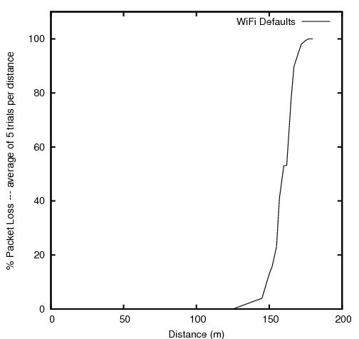
In the example above, the test suite checking the ns-3 wireless device propagation loss models failed. By default no further information is provided.

To further explore the failure, test.py allows a single test suite to be specified. Running the command

$ ./test.py --suite=ns3-wifi-propagation-loss-models

or equivalently

$ ./test.py -s ns3-wifi-propagation-loss-models

results in that single test suite being run.

FAIL: TestSuite ns3-wifi-propagation-loss-models

To find detailed information regarding the failure, one must specify the kind of output desired. For example, most people will probably be interested in a text file:

$ ./test.py --suite=ns3-wifi-propagation-loss-models --text=results.txt

This will result in that single test suite being run with the test status written to the file ‘’results.txt’‘.

You should find something similar to the following in that file

FAIL: Test Suite ''ns3-wifi-propagation-loss-models'' (real 0.02 user 0.01 system 0.00)
PASS: Test Case "Check ... Friis ... model ..." (real 0.01 user 0.00 system 0.00)
FAIL: Test Case "Check ... Log Distance ... model" (real 0.01 user 0.01 system 0.00)
  Details:
    Message:   Got unexpected SNR value
    Condition: [long description of what actually failed]
    Actual:    176.395
    Limit:     176.407 +- 0.0005
    File:      ../src/test/ns3wifi/propagation-loss-models-test-suite.cc
    Line:      360

Notice that the Test Suite is composed of two Test Cases. The first test case checked the Friis propagation loss model and passed. The second test case failed checking the Log Distance propagation model. In this case, an SNR of 176.395 was found, and the test expected a value of 176.407 correct to three decimal places. The file which implemented the failing test is listed as well as the line of code which triggered the failure.

If you desire, you could just as easily have written an HTML file using the --html option as described above.

Typically a user will run all tests at least once after downloading ns-3 to ensure that his or her environment has been built correctly and is generating correct results according to the test suites. Developers will typically run the test suites before and after making a change to ensure that they have not introduced a regression with their changes. In this case, developers may not want to run all tests, but only a subset. For example, the developer might only want to run the unit tests periodically while making changes to a repository. In this case, test.py can be told to constrain the types of tests being run to a particular class of tests. The following command will result in only the unit tests being run:

$ ./test.py --constrain=unit

Similarly, the following command will result in only the example smoke tests being run:

$ ./test.py --constrain=unit

To see a quick list of the legal kinds of constraints, you can ask for them to be listed. The following command

$ ./test.py --kinds

will result in the following list being displayed:

Waf: Entering directory `/home/craigdo/repos/ns-3-allinone-test/ns-3-dev/build'
Waf: Leaving directory `/home/craigdo/repos/ns-3-allinone-test/ns-3-dev/build'
'build' finished successfully (0.939s)Waf: Entering directory `/home/craigdo/repos/ns-3-allinone-test/ns-3-dev/build'
bvt:         Build Verification Tests (to see if build completed successfully)
core:        Run all TestSuite-based tests (exclude examples)
example:     Examples (to see if example programs run successfully)
performance: Performance Tests (check to see if the system is as fast as expected)
system:      System Tests (spans modules to check integration of modules)
unit:        Unit Tests (within modules to check basic functionality)

Any of these kinds of test can be provided as a constraint using the --constraint option.

To see a quick list of all of the test suites available, you can ask for them to be listed. The following command,

$ ./test.py --list

will result in a list of the test suite being displayed, similar to

Waf: Entering directory `/home/craigdo/repos/ns-3-allinone-test/ns-3-dev/build'
Waf: Leaving directory `/home/craigdo/repos/ns-3-allinone-test/ns-3-dev/build'
'build' finished successfully (0.939s)
histogram
ns3-wifi-interference
ns3-tcp-cwnd
ns3-tcp-interoperability
sample
devices-mesh-flame
devices-mesh-dot11s
devices-mesh
...
object-name-service
callback
attributes
config
global-value
command-line
basic-random-number
object

Any of these listed suites can be selected to be run by itself using the --suite option as shown above.

Similarly to test suites, one can run a single C++ example program using the --example option. Note that the relative path for the example does not need to be included and that the executables built for C++ examples do not have extensions. Entering

$ ./test.py --example=udp-echo

results in that single example being run.

PASS: Example examples/udp/udp-echo

You can specify the directory where ns-3 was built using the --buildpath option as follows.

$ ./test.py --buildpath=/home/craigdo/repos/ns-3-allinone-test/ns-3-dev/build/debug --example=wifi-simple-adhoc

One can run a single Python example program using the --pyexample option. Note that the relative path for the example must be included and that Python examples do need their extensions. Entering

$ ./test.py --pyexample=examples/tutorial/first.py

results in that single example being run.

PASS: Example examples/tutorial/first.py

Because Python examples are not built, you do not need to specify the directory where ns-3 was built to run them.

Normally when example programs are executed, they write a large amount of trace file data. This is normally saved to the base directory of the distribution (e.g., /home/user/ns-3-dev). When test.py runs an example, it really is completely unconcerned with the trace files. It just wants to to determine if the example can be built and run without error. Since this is the case, the trace files are written into a /tmp/unchecked-traces directory. If you run the above example, you should be able to find the associated udp-echo.tr and udp-echo-n-1.pcap files there.

The list of available examples is defined by the contents of the ‘’examples’’ directory in the distribution. If you select an example for execution using the --example option, test.py will not make any attempt to decide if the example has been configured or not, it will just try to run it and report the result of the attempt.

When test.py runs, by default it will first ensure that the system has been completely built. This can be defeated by selecting the --nowaf option.

$ ./test.py --list --nowaf

will result in a list of the currently built test suites being displayed, similar to:

ns3-wifi-propagation-loss-models
ns3-tcp-cwnd
ns3-tcp-interoperability
pcap-file-object
object-name-service
random-number-generators

Note the absence of the Waf build messages.

test.py also supports running the test suites and examples under valgrind. Valgrind is a flexible program for debugging and profiling Linux executables. By default, valgrind runs a tool called memcheck, which performs a range of memory- checking functions, including detecting accesses to uninitialised memory, misuse of allocated memory (double frees, access after free, etc.) and detecting memory leaks. This can be selected by using the --grind option.

$ ./test.py --grind

As it runs, test.py and the programs that it runs indirectly, generate large numbers of temporary files. Usually, the content of these files is not interesting, however in some cases it can be useful (for debugging purposes) to view these files. test.py provides a --retain option which will cause these temporary files to be kept after the run is completed. The files are saved in a directory named testpy-output under a subdirectory named according to the current Coordinated Universal Time (also known as Greenwich Mean Time).

$ ./test.py --retain

Finally, test.py provides a --verbose option which will print large amounts of information about its progress. It is not expected that this will be terribly useful unless there is an error. In this case, you can get access to the standard output and standard error reported by running test suites and examples. Select verbose in the following way:

$ ./test.py --verbose

All of these options can be mixed and matched. For example, to run all of the ns-3 core test suites under valgrind, in verbose mode, while generating an HTML output file, one would do:

$ ./test.py --verbose --grind --constrain=core --html=results.html

TestTaxonomy

As mentioned above, tests are grouped into a number of broadly defined classifications to allow users to selectively run tests to address the different kinds of testing that need to be done.

  • Build Verification Tests
  • Unit Tests
  • System Tests
  • Examples
  • Performance Tests
BuildVerificationTests

These are relatively simple tests that are built along with the distribution and are used to make sure that the build is pretty much working. Our current unit tests live in the source files of the code they test and are built into the ns-3 modules; and so fit the description of BVTs. BVTs live in the same source code that is built into the ns-3 code. Our current tests are examples of this kind of test.

Unit Tests

Unit tests are more involved tests that go into detail to make sure that a piece of code works as advertised in isolation. There is really no reason for this kind of test to be built into an ns-3 module. It turns out, for example, that the unit tests for the object name service are about the same size as the object name service code itself. Unit tests are tests that check a single bit of functionality that are not built into the ns-3 code, but live in the same directory as the code it tests. It is possible that these tests check integration of multiple implementation files in a module as well. The file src/core/test/names-test-suite.cc is an example of this kind of test. The file src/network/test/pcap-file-test-suite.cc is another example that uses a known good pcap file as a test vector file. This file is stored locally in the src/network directory.

System Tests

System tests are those that involve more than one module in the system. We have lots of this kind of test running in our current regression framework, but they are typically overloaded examples. We provide a new place for this kind of test in the directory src/test. The file src/test/ns3tcp/ns3-interop-test-suite.cc is an example of this kind of test. It uses NSC TCP to test the ns-3 TCP implementation. Often there will be test vectors required for this kind of test, and they are stored in the directory where the test lives. For example, ns3tcp-interop-response-vectors.pcap is a file consisting of a number of TCP headers that are used as the expected responses of the ns-3 TCP under test to a stimulus generated by the NSC TCP which is used as a ‘’known good’’ implementation.

Examples

The examples are tested by the framework to make sure they built and will run. Nothing is checked, and currently the pcap files are just written off into /tmp to be discarded. If the examples run (don’t crash) they pass this smoke test.

Performance Tests

Performance tests are those which exercise a particular part of the system and determine if the tests have executed to completion in a reasonable time.

Running Tests

Tests are typically run using the high level test.py program. To get a list of the available command-line options, run test.py --help

The test program test.py will run both tests and those examples that have been added to the list to check. The difference between tests and examples is as follows. Tests generally check that specific simulation output or events conforms to expected behavior. In contrast, the output of examples is not checked, and the test program merely checks the exit status of the example program to make sure that it runs without error.

Briefly, to run all tests, first one must configure tests during configuration stage, and also (optionally) examples if examples are to be checked:

$ ./waf --configure --enable-examples --enable-tests

Then, build ns-3, and after it is built, just run test.py. test.py -h will show a number of configuration options that modify the behavior of test.py.

The program test.py invokes, for C++ tests and examples, a lower-level C++ program called test-runner to actually run the tests. As discussed below, this test-runner can be a helpful way to debug tests.

Debugging Tests

The debugging of the test programs is best performed running the low-level test-runner program. The test-runner is the bridge from generic Python code to ns-3 code. It is written in C++ and uses the automatic test discovery process in the ns-3 code to find and allow execution of all of the various tests.

The main reason why test.py is not suitable for debugging is that it is not allowed for logging to be turned on using the NS_LOG environmental variable when test.py runs. This limitation does not apply to the test-runner executable. Hence, if you want to see logging output from your tests, you have to run them using the test-runner directly.

In order to execute the test-runner, you run it like any other ns-3 executable – using waf. To get a list of available options, you can type:

$ ./waf --run "test-runner --help"

You should see something like the following

Waf: Entering directory `/home/craigdo/repos/ns-3-allinone-test/ns-3-dev/build'
Waf: Leaving directory `/home/craigdo/repos/ns-3-allinone-test/ns-3-dev/build'
'build' finished successfully (0.353s)
--assert:               Tell tests to segfault (like assert) if an error is detected
--basedir=dir:          Set the base directory (where to find src) to ''dir''
--tempdir=dir:          Set the temporary directory (where to find data files) to ''dir''
--constrain=test-type:  Constrain checks to test suites of type ''test-type''
--help:                 Print this message
--kinds:                List all of the available kinds of tests
--list:                 List all of the test suites (optionally constrained by test-type)
--out=file-name:        Set the test status output file to ''file-name''
--suite=suite-name:     Run the test suite named ''suite-name''
--verbose:              Turn on messages in the run test suites

There are a number of things available to you which will be familiar to you if you have looked at test.py. This should be expected since the test- runner is just an interface between test.py and ns-3. You may notice that example-related commands are missing here. That is because the examples are really not ns-3 tests. test.py runs them as if they were to present a unified testing environment, but they are really completely different and not to be found here.

The first new option that appears here, but not in test.py is the --assert option. This option is useful when debugging a test case when running under a debugger like gdb. When selected, this option tells the underlying test case to cause a segmentation violation if an error is detected. This has the nice side-effect of causing program execution to stop (break into the debugger) when an error is detected. If you are using gdb, you could use this option something like,

$ ./waf shell
$ cd build/debug/utils
$ gdb test-runner
$ run --suite=global-value --assert

If an error is then found in the global-value test suite, a segfault would be generated and the (source level) debugger would stop at the NS_TEST_ASSERT_MSG that detected the error.

Another new option that appears here is the --basedir option. It turns out that some tests may need to reference the source directory of the ns-3 distribution to find local data, so a base directory is always required to run a test.

If you run a test from test.py, the Python program will provide the basedir option for you. To run one of the tests directly from the test-runner using waf, you will need to specify the test suite to run along with the base directory. So you could use the shell and do:

$ ./waf --run "test-runner --basedir=`pwd` --suite=pcap-file-object"

Note the ‘’backward’’ quotation marks on the pwd command.

If you are running the test suite out of a debugger, it can be quite painful to remember and constantly type the absolute path of the distribution base directory. Because of this, if you omit the basedir, the test-runner will try to figure one out for you. It begins in the current working directory and walks up the directory tree looking for a directory file with files named VERSION and LICENSE. If it finds one, it assumes that must be the basedir and provides it for you.

Test output

Many test suites need to write temporary files (such as pcap files) in the process of running the tests. The tests then need a temporary directory to write to. The Python test utility (test.py) will provide a temporary file automatically, but if run stand-alone this temporary directory must be provided. Just as in the basedir case, it can be annoying to continually have to provide a --tempdir, so the test runner will figure one out for you if you don’t provide one. It first looks for environment variables named TMP and TEMP and uses those. If neither TMP nor TEMP are defined it picks /tmp. The code then tacks on an identifier indicating what created the directory (ns-3) then the time (hh.mm.ss) followed by a large random number. The test runner creates a directory of that name to be used as the temporary directory. Temporary files then go into a directory that will be named something like

/tmp/ns-3.10.25.37.61537845

The time is provided as a hint so that you can relatively easily reconstruct what directory was used if you need to go back and look at the files that were placed in that directory.

Another class of output is test output like pcap traces that are generated to compare to reference output. The test program will typically delete these after the test suites all run. To disable the deletion of test output, run test.py with the “retain” option:

$ ./test.py -r

and test output can be found in the testpy-output/ directory.

Reporting of test failures

When you run a test suite using the test-runner it will run the test quietly by default. The only indication that you will get that the test passed is the absence of a message from waf saying that the program returned something other than a zero exit code. To get some output from the test, you need to specify an output file to which the tests will write their XML status using the --out option. You need to be careful interpreting the results because the test suites will append results onto this file. Try,

$ ./waf --run "test-runner --basedir=`pwd` --suite=pcap-file-object --out=myfile.xml"

If you look at the file myfile.xml you should see something like,

<TestSuite>
  <SuiteName>pcap-file-object</SuiteName>
  <TestCase>
    <CaseName>Check to see that PcapFile::Open with mode ''w'' works</CaseName>
    <CaseResult>PASS</CaseResult>
    <CaseTime>real 0.00 user 0.00 system 0.00</CaseTime>
  </TestCase>
  <TestCase>
    <CaseName>Check to see that PcapFile::Open with mode ''r'' works</CaseName>
    <CaseResult>PASS</CaseResult>
    <CaseTime>real 0.00 user 0.00 system 0.00</CaseTime>
  </TestCase>
  <TestCase>
    <CaseName>Check to see that PcapFile::Open with mode ''a'' works</CaseName>
    <CaseResult>PASS</CaseResult>
    <CaseTime>real 0.00 user 0.00 system 0.00</CaseTime>
  </TestCase>
  <TestCase>
    <CaseName>Check to see that PcapFileHeader is managed correctly</CaseName>
    <CaseResult>PASS</CaseResult>
    <CaseTime>real 0.00 user 0.00 system 0.00</CaseTime>
  </TestCase>
  <TestCase>
    <CaseName>Check to see that PcapRecordHeader is managed correctly</CaseName>
    <CaseResult>PASS</CaseResult>
    <CaseTime>real 0.00 user 0.00 system 0.00</CaseTime>
  </TestCase>
  <TestCase>
    <CaseName>Check to see that PcapFile can read out a known good pcap file</CaseName>
    <CaseResult>PASS</CaseResult>
    <CaseTime>real 0.00 user 0.00 system 0.00</CaseTime>
  </TestCase>
  <SuiteResult>PASS</SuiteResult>
  <SuiteTime>real 0.00 user 0.00 system 0.00</SuiteTime>
</TestSuite>

If you are familiar with XML this should be fairly self-explanatory. It is also not a complete XML file since test suites are designed to have their output appended to a master XML status file as described in the test.py section.

Debugging test suite failures

To debug test crashes, such as

CRASH: TestSuite ns3-wifi-interference

You can access the underlying test-runner program via gdb as follows, and then pass the “–basedir=`pwd`” argument to run (you can also pass other arguments as needed, but basedir is the minimum needed):

$ ./waf --command-template="gdb %s" --run "test-runner"
Waf: Entering directory `/home/tomh/hg/sep09/ns-3-allinone/ns-3-dev-678/build'
Waf: Leaving directory `/home/tomh/hg/sep09/ns-3-allinone/ns-3-dev-678/build'
'build' finished successfully (0.380s)
GNU gdb 6.8-debian
Copyright (C) 2008 Free Software Foundation, Inc.
L cense GPLv3+: GNU GPL version 3 or later <http://gnu.org/licenses/gpl.html>
This is free software: you are free to change and redistribute it.
There is NO WARRANTY, to the extent permitted by law.  Type "show copying"
and "show warranty" for details.
This GDB was configured as "x86_64-linux-gnu"...
(gdb) r --basedir=`pwd`
Starting program: <..>/build/debug/utils/test-runner --basedir=`pwd`
[Thread debugging using libthread_db enabled]
assert failed. file=../src/core/model/type-id.cc, line=138, cond="uid <= m_information.size () && uid != 0"
...

Here is another example of how to use valgrind to debug a memory problem such as:

VALGR: TestSuite devices-mesh-dot11s-regression

$ ./waf --command-template="valgrind %s --basedir=`pwd` --suite=devices-mesh-dot11s-regression" --run test-runner

Class TestRunner

The executables that run dedicated test programs use a TestRunner class. This class provides for automatic test registration and listing, as well as a way to execute the individual tests. Individual test suites use C++ global constructors to add themselves to a collection of test suites managed by the test runner. The test runner is used to list all of the available tests and to select a test to be run. This is a quite simple class that provides three static methods to provide or Adding and Getting test suites to a collection of tests. See the doxygen for class ns3::TestRunner for details.

Test Suite

All ns-3 tests are classified into Test Suites and Test Cases. A test suite is a collection of test cases that completely exercise a given kind of functionality. As described above, test suites can be classified as,

  • Build Verification Tests
  • Unit Tests
  • System Tests
  • Examples
  • Performance Tests

This classification is exported from the TestSuite class. This class is quite simple, existing only as a place to export this type and to accumulate test cases. From a user perspective, in order to create a new TestSuite in the system one only has to define a new class that inherits from class TestSuite and perform these two duties.

The following code will define a new class that can be run by test.py as a ‘’unit’’ test with the display name, my-test-suite-name.

class MySuite : public TestSuite
{
public:
  MyTestSuite ();
};

MyTestSuite::MyTestSuite ()
  : TestSuite ("my-test-suite-name", UNIT)
{
  AddTestCase (new MyTestCase);
}

MyTestSuite myTestSuite;

The base class takes care of all of the registration and reporting required to be a good citizen in the test framework.

Test Case

Individual tests are created using a TestCase class. Common models for the use of a test case include “one test case per feature”, and “one test case per method.” Mixtures of these models may be used.

In order to create a new test case in the system, all one has to do is to inherit from the TestCase base class, override the constructor to give the test case a name and override the DoRun method to run the test.

class MyTestCase : public TestCase
{
  MyTestCase ();
  virtual void DoRun (void);
};

MyTestCase::MyTestCase ()
  : TestCase ("Check some bit of functionality")
{
}

void
MyTestCase::DoRun (void)
{
  NS_TEST_ASSERT_MSG_EQ (true, true, "Some failure message");
}

Utilities

There are a number of utilities of various kinds that are also part of the testing framework. Examples include a generalized pcap file useful for storing test vectors; a generic container useful for transient storage of test vectors during test execution; and tools for generating presentations based on validation and verification testing results.

These utilities are not documented here, but for example, please see how the TCP tests found in src/test/ns3tcp/ use pcap files and reference output.

How to write tests

A primary goal of the ns-3 project is to help users to improve the validity and credibility of their results. There are many elements to obtaining valid models and simulations, and testing is a major component. If you contribute models or examples to ns-3, you may be asked to contribute test code. Models that you contribute will be used for many years by other people, who probably have no idea upon first glance whether the model is correct. The test code that you write for your model will help to avoid future regressions in the output and will aid future users in understanding the verification and bounds of applicability of your models.

There are many ways to verify the correctness of a model’s implementation. In this section, we hope to cover some common cases that can be used as a guide to writing new tests.

Sample TestSuite skeleton

When starting from scratch (i.e. not adding a TestCase to an existing TestSuite), these things need to be decided up front:

  • What the test suite will be called
  • What type of test it will be (Build Verification Test, Unit Test, System Test, or Performance Test)
  • Where the test code will live (either in an existing ns-3 module or separately in src/test/ directory). You will have to edit the wscript file in that directory to compile your new code, if it is a new file.

A program called src/create-module.py is a good starting point. This program can be invoked such as create-module.py router for a hypothetical new module called router. Once you do this, you will see a router directory, and a test/router-test-suite.cc test suite. This file can be a starting point for your initial test. This is a working test suite, although the actual tests performed are trivial. Copy it over to your module’s test directory, and do a global substitution of “Router” in that file for something pertaining to the model that you want to test. You can also edit things such as a more descriptive test case name.

You also need to add a block into your wscript to get this test to compile:

module_test.source = [
    'test/router-test-suite.cc',
    ]

Before you actually start making this do useful things, it may help to try to run the skeleton. Make sure that ns-3 has been configured with the “–enable-tests” option. Let’s assume that your new test suite is called “router” such as here:

RouterTestSuite::RouterTestSuite ()
  : TestSuite ("router", UNIT)

Try this command:

$ ./test.py -s router

Output such as below should be produced:

PASS: TestSuite router
1 of 1 tests passed (1 passed, 0 skipped, 0 failed, 0 crashed, 0 valgrind errors)

See src/lte/test/test-lte-antenna.cc for a worked example.

Test macros

There are a number of macros available for checking test program output with expected output. These macros are defined in src/core/model/test.h.

The main set of macros that are used include the following:

NS_TEST_ASSERT_MSG_EQ(actual, limit, msg)
NS_TEST_ASSERT_MSG_NE(actual, limit, msg)
NS_TEST_ASSERT_MSG_LT(actual, limit, msg)
NS_TEST_ASSERT_MSG_GT(actual, limit, msg)
NS_TEST_ASSERT_MSG_EQ_TOL(actual, limit, tol, msg)

The first argument actual is the value under test, the second value limit is the expected value (or the value to test against), and the last argument msg is the error message to print out if the test fails.

The first four macros above test for equality, inequality, less than, or greater than, respectively. The fifth macro above tests for equality, but within a certain tolerance. This variant is useful when testing floating point numbers for equality against a limit, where you want to avoid a test failure due to rounding errors.

Finally, there are variants of the above where the keyword ASSERT is replaced by EXPECT. These variants are designed specially for use in methods (especially callbacks) returning void. Reserve their use for callbacks that you use in your test programs; otherwise, use the ASSERT variants.

How to add an example program to the test suite

One can “smoke test” that examples compile and run successfully to completion (without memory leaks) using the examples-to-run.py script located in your module’s test directory. Briefly, by including an instance of this file in your test directory, you can cause the test runner to execute the examples listed. It is usually best to make sure that you select examples that have reasonably short run times so as to not bog down the tests. See the example in src/lte/test/ directory.

Testing for boolean outcomes

Testing outcomes when randomness is involved

Testing output data against a known distribution

Providing non-trivial input vectors of data

Storing and referencing non-trivial output data

Presenting your output test data

Support

Creating a new ns-3 model

This chapter walks through the design process of an ns-3 model. In many research cases, users will not be satisfied to merely adapt existing models, but may want to extend the core of the simulator in a novel way. We will use the example of adding an ErrorModel to a simple ns-3 link as a motivating example of how one might approach this problem and proceed through a design and implementation.

Note

Documentation

Here we focus on the process of creating new models and new modules, and some of the design choices involved. For the sake of clarity, we defer discussion of the mechanics of documenting models and source code to the Documentation chapter.

Design Approach

Consider how you want it to work; what should it do. Think about these things:

  • functionality: What functionality should it have? What attributes or configuration is exposed to the user?
  • reusability: How much should others be able to reuse my design? Can I reuse code from ns-2 to get started? How does a user integrate the model with the rest of another simulation?
  • dependencies: How can I reduce the introduction of outside dependencies on my new code as much as possible (to make it more modular)? For instance, should I avoid any dependence on IPv4 if I want it to also be used by IPv6? Should I avoid any dependency on IP at all?

Do not be hesitant to contact the ns-3-users or ns-developers list if you have questions. In particular, it is important to think about the public API of your new model and ask for feedback. It also helps to let others know of your work in case you are interested in collaborators.

Example: ErrorModel

An error model exists in ns-2. It allows packets to be passed to a stateful object that determines, based on a random variable, whether the packet is corrupted. The caller can then decide what to do with the packet (drop it, etc.).

The main API of the error model is a function to pass a packet to, and the return value of this function is a boolean that tells the caller whether any corruption occurred. Note that depending on the error model, the packet data buffer may or may not be corrupted. Let’s call this function “IsCorrupt()”.

So far, in our design, we have:

class ErrorModel
{
public:
 /**
  * \returns true if the Packet is to be considered as errored/corrupted
  * \param pkt Packet to apply error model to
  */
  bool IsCorrupt (Ptr<Packet> pkt);
};

Note that we do not pass a const pointer, thereby allowing the function to modify the packet if IsCorrupt() returns true. Not all error models will actually modify the packet; whether or not the packet data buffer is corrupted should be documented.

We may also want specialized versions of this, such as in ns-2, so although it is not the only design choice for polymorphism, we assume that we will subclass a base class ErrorModel for specialized classes, such as RateErrorModel, ListErrorModel, etc, such as is done in ns-2.

You may be thinking at this point, “Why not make IsCorrupt() a virtual method?”. That is one approach; the other is to make the public non-virtual function indirect through a private virtual function (this in C++ is known as the non virtual interface idiom and is adopted in the ns-3 ErrorModel class).

Next, should this device have any dependencies on IP or other protocols? We do not want to create dependencies on Internet protocols (the error model should be applicable to non-Internet protocols too), so we’ll keep that in mind later.

Another consideration is how objects will include this error model. We envision putting an explicit setter in certain NetDevice implementations, for example.:

/**
 * Attach a receive ErrorModel to the PointToPointNetDevice.
 *
 * The PointToPointNetDevice may optionally include an ErrorModel in
 * the packet receive chain.
 *
 * @see ErrorModel
 * @param em Ptr to the ErrorModel.
 */
void PointToPointNetDevice::SetReceiveErrorModel(Ptr<ErrorModel> em);

Again, this is not the only choice we have (error models could be aggregated to lots of other objects), but it satisfies our primary use case, which is to allow a user to force errors on otherwise successful packet transmissions, at the NetDevice level.

After some thinking and looking at existing ns-2 code, here is a sample API of a base class and first subclass that could be posted for initial review:

class ErrorModel
{
public:
  ErrorModel ();
  virtual ~ErrorModel ();
  bool IsCorrupt (Ptr<Packet> pkt);
  void Reset (void);
  void Enable (void);
  void Disable (void);
  bool IsEnabled (void) const;
private:
  virtual bool DoCorrupt (Ptr<Packet> pkt) = 0;
  virtual void DoReset (void) = 0;
};

enum ErrorUnit
  {
    EU_BIT,
    EU_BYTE,
    EU_PKT
  };

// Determine which packets are errored corresponding to an underlying
// random variable distribution, an error rate, and unit for the rate.
class RateErrorModel : public ErrorModel
{
public:
  RateErrorModel ();
  virtual ~RateErrorModel ();
  enum ErrorUnit GetUnit (void) const;
  void SetUnit (enum ErrorUnit error_unit);
  double GetRate (void) const;
  void SetRate (double rate);
  void SetRandomVariable (const RandomVariable &ranvar);
private:
  virtual bool DoCorrupt (Ptr<Packet> pkt);
  virtual void DoReset (void);
};

Scaffolding

Let’s say that you are ready to start implementing; you have a fairly clear picture of what you want to build, and you may have solicited some initial review or suggestions from the list. One way to approach the next step (implementation) is to create scaffolding and fill in the details as the design matures.

This section walks through many of the steps you should consider to define scaffolding, or a non-functional skeleton of what your model will eventually implement. It is usually good practice to not wait to get these details integrated at the end, but instead to plumb a skeleton of your model into the system early and then add functions later once the API and integration seems about right.

Note that you will want to modify a few things in the below presentation for your model since if you follow the error model verbatim, the code you produce will collide with the existing error model. The below is just an outline of how ErrorModel was built that you can adapt to other models.

Review the ns-3 Coding Style Document

At this point, you may want to pause and read the ns-3 coding style document, especially if you are considering to contribute your code back to the project. The coding style document is linked off the main project page: ns-3 coding style.

Decide Where in the Source Tree the Model Should Reside

All of the ns-3 model source code is in the directory src/. You will need to choose which subdirectory it resides in. If it is new model code of some sort, it makes sense to put it into the src/ directory somewhere, particularly for ease of integrating with the build system.

In the case of the error model, it is very related to the packet class, so it makes sense to implement this in the src/network/ module where ns-3 packets are implemented.

waf and wscript

ns-3 uses the Waf build system. You will want to integrate your new ns-3 uses the Waf build system. You will want to integrate your new source files into this system. This requires that you add your files to the wscript file found in each directory.

Let’s start with empty files error-model.h and error-model.cc, and add this to src/network/wscript. It is really just a matter of adding the .cc file to the rest of the source files, and the .h file to the list of the header files.

Now, pop up to the top level directory and type ”./test.py”. You shouldn’t have broken anything by this operation.

Include Guards

Next, let’s add some include guards in our header file.:

#ifndef ERROR_MODEL_H
#define ERROR_MODEL_H
...
#endif
namespace ns3

ns-3 uses the ns-3 namespace to isolate its symbols from other namespaces. Typically, a user will next put an ns-3 namespace block in both the cc and h file.:

namespace ns3 {
...
}

At this point, we have some skeletal files in which we can start defining our new classes. The header file looks like this:

#ifndef ERROR_MODEL_H
#define ERROR_MODEL_H

namespace ns3 {

} // namespace ns3
#endif

while the error-model.cc file simply looks like this:

#include "error-model.h"

namespace ns3 {

} // namespace ns3

These files should compile since they don’t really have any contents. We’re now ready to start adding classes.

Initial Implementation

At this point, we’re still working on some scaffolding, but we can begin to define our classes, with the functionality to be added later.

Inherit from the Object Class?

This is an important design step; whether to use class Object as a base class for your new classes.

As described in the chapter on the ns-3 Object model, classes that inherit from class Object get special properties:

  • the ns-3 type and attribute system (see Configuration and Attributes)
  • an object aggregation system
  • a smart-pointer reference counting system (class Ptr)

Classes that derive from class ObjectBase} get the first two properties above, but do not get smart pointers. Classes that derive from class RefCountBase get only the smart-pointer reference counting system.

In practice, class Object is the variant of the three above that the ns-3 developer will most commonly encounter.

In our case, we want to make use of the attribute system, and we will be passing instances of this object across the ns-3 public API, so class Object is appropriate for us.

Initial Classes

One way to proceed is to start by defining the bare minimum functions and see if they will compile. Let’s review what all is needed to implement when we derive from class Object.:

#ifndef ERROR_MODEL_H
#define ERROR_MODEL_H

#include "ns3/object.h"

namespace ns3 {

class ErrorModel : public Object
{
public:
  static TypeId GetTypeId (void);

  ErrorModel ();
  virtual ~ErrorModel ();
};

class RateErrorModel : public ErrorModel
{
public:
  static TypeId GetTypeId (void);

  RateErrorModel ();
  virtual ~RateErrorModel ();
};
#endif

A few things to note here. We need to include object.h. The convention in ns-3 is that if the header file is co-located in the same directory, it may be included without any path prefix. Therefore, if we were implementing ErrorModel in src/core/model directory, we could have just said “#include "object.h"”. But we are in src/network/model, so we must include it as “#include "ns3/object.h"”. Note also that this goes outside the namespace declaration.

Second, each class must implement a static public member function called GetTypeId (void).

Third, it is a good idea to implement constructors and destructors rather than to let the compiler generate them, and to make the destructor virtual. In C++, note also that copy assignment operator and copy constructors are auto-generated if they are not defined, so if you do not want those, you should implement those as private members. This aspect of C++ is discussed in Scott Meyers’ Effective C++ book. item 45.

Let’s now look at some corresponding skeletal implementation code in the .cc file.:

#include "error-model.h"

namespace ns3 {

NS_OBJECT_ENSURE_REGISTERED (ErrorModel);

TypeId ErrorModel::GetTypeId (void)
{
  static TypeId tid = TypeId ("ns3::ErrorModel")
    .SetParent<Object> ()
    ;
  return tid;
}

ErrorModel::ErrorModel ()
{
}

ErrorModel::~ErrorModel ()
{
}

NS_OBJECT_ENSURE_REGISTERED (RateErrorModel);

TypeId RateErrorModel::GetTypeId (void)
{
  static TypeId tid = TypeId ("ns3::RateErrorModel")
    .SetParent<ErrorModel> ()
    .AddConstructor<RateErrorModel> ()
    ;
  return tid;
}

RateErrorModel::RateErrorModel ()
{
}

RateErrorModel::~RateErrorModel ()
{
}

What is the GetTypeId (void) function? This function does a few things. It registers a unique string into the TypeId system. It establishes the hierarchy of objects in the attribute system (via SetParent). It also declares that certain objects can be created via the object creation framework (AddConstructor).

The macro NS_OBJECT_ENSURE_REGISTERED (classname) is needed also once for every class that defines a new GetTypeId method, and it does the actual registration of the class into the system. The Object model chapter discusses this in more detail.

Including External Files
Logging Support

Here, write a bit about adding |ns3| logging macros. Note that LOG_COMPONENT_DEFINE is done outside the namespace ns3

Constructor, Empty Function Prototypes
Key Variables (Default Values, Attributes)
Test Program 1
Object Framework

Adding a Sample Script

At this point, one may want to try to take the basic scaffolding defined above and add it into the system. Performing this step now allows one to use a simpler model when plumbing into the system and may also reveal whether any design or API modifications need to be made. Once this is done, we will return to building out the functionality of the ErrorModels themselves.

Add Basic Support in the Class
/* point-to-point-net-device.h */
  class ErrorModel;

  /**
   * Error model for receive packet events
   */
  Ptr<ErrorModel> m_receiveErrorModel;
Add Accessor
void
PointToPointNetDevice::SetReceiveErrorModel (Ptr<ErrorModel> em)
{
  NS_LOG_FUNCTION (this << em);
  m_receiveErrorModel = em;
}

   .AddAttribute ("ReceiveErrorModel",
                   "The receiver error model used to simulate packet loss",
                   PointerValue (),
                   MakePointerAccessor (&PointToPointNetDevice::m_receiveErrorModel),
                   MakePointerChecker<ErrorModel> ())
Plumb Into the System
void PointToPointNetDevice::Receive (Ptr<Packet> packet)
{
  NS_LOG_FUNCTION (this << packet);
  uint16_t protocol = 0;

  if (m_receiveErrorModel && m_receiveErrorModel->IsCorrupt (packet) )
    {
//
// If we have an error model and it indicates that it is time to lose a
// corrupted packet, don't forward this packet up, let it go.
//
      m_dropTrace (packet);
    }
  else
    {
//
// Hit the receive trace hook, strip off the point-to-point protocol header
// and forward this packet up the protocol stack.
//
      m_rxTrace (packet);
      ProcessHeader(packet, protocol);
      m_rxCallback (this, packet, protocol, GetRemote ());
      if (!m_promiscCallback.IsNull ())
        {           m_promiscCallback (this, packet, protocol, GetRemote (),
                      GetAddress (), NetDevice::PACKET_HOST);
        }
    }
}
Create Null Functional Script
/* simple-error-model.cc */

  // Error model
  // We want to add an error model to node 3's NetDevice
  // We can obtain a handle to the NetDevice via the channel and node
  // pointers
  Ptr<PointToPointNetDevice> nd3 = PointToPointTopology::GetNetDevice
    (n3, channel2);
  Ptr<ErrorModel> em = Create<ErrorModel> ();
  nd3->SetReceiveErrorModel (em);


bool
ErrorModel::DoCorrupt (Packet& p)
{
  NS_LOG_FUNCTION;
  NS_LOG_UNCOND("Corrupt!");
  return false;
}

At this point, we can run the program with our trivial ErrorModel plumbed into the receive path of the PointToPointNetDevice. It prints out the string “Corrupt!” for each packet received at node n3. Next, we return to the error model to add in a subclass that performs more interesting error modeling.

Add a Subclass

The trivial base class ErrorModel does not do anything interesting, but it provides a useful base class interface (Corrupt () and Reset ()), forwarded to virtual functions that can be subclassed. Let’s next consider what we call a BasicErrorModel which is based on the ns-2 ErrorModel class (in ns-2/queue/errmodel.{cc,h}).

What properties do we want this to have, from a user interface perspective? We would like for the user to be able to trivially swap out the type of ErrorModel used in the NetDevice. We would also like the capability to set configurable parameters.

Here are a few simple requirements we will consider:

  • Ability to set the random variable that governs the losses (default is UniformVariable)
  • Ability to set the unit (bit, byte, packet, time) of granularity over which errors are applied.
  • Ability to set the rate of errors (e.g. 10^-3) corresponding to the above unit of granularity.
  • Ability to enable/disable (default is enabled)
How to Subclass

We declare BasicErrorModel to be a subclass of ErrorModel as follows,:

class BasicErrorModel : public ErrorModel
{
public:
  static TypeId GetTypeId (void);
  ...
private:
  // Implement base class pure virtual functions
  virtual bool DoCorrupt (Ptr<Packet> p);
  virtual bool DoReset (void);
  ...
}

and configure the subclass GetTypeId function by setting a unique TypeId string and setting the Parent to ErrorModel:

TypeId RateErrorModel::GetTypeId (void)
{
  static TypeId tid = TypeId ("ns3::RateErrorModel")
    .SetParent<ErrorModel> ()
    .AddConstructor<RateErrorModel> ()
  ...

Build Core Functions and Unit Tests

Assert Macros
Writing Unit Tests

Adding a New Module to ns-3

When you have created a group of related classes, examples, and tests, they can be combined together into an ns-3 module so that they can be used with existing ns-3 modules and by other researchers.

This chapter walks you through the steps necessary to add a new module to ns-3.

Step 1 - Familiarize yourself with the module layout

All modules can be found in the src directory. Each module can be found in a directory that has the same name as the module. For example, the spectrum module can be found here:

src/spectrum

A prototypical module has the following directory structure and required files:

src/
      module-name/
              bindings/
              doc/
              examples/
                      wscript
              helper/
              model/
              test/
                      examples-to-run.py
              wscript

Not all directories will be present in each module.

Step 2 - Create your new module based on the template module

A python program is provided in the source directory that will create a skeleton for a new module

$ src/create-module.py

For the purposes of this discussion we will assume that your new module is called “new-module”. From the src directory, do the following to create the new module:

$ ./create-module.py new-module

Next, cd into new-module; you will find this directory layout:

$ examples  helper  model  test  wscript

We next walk through how to customize this module. All ns-3 modules depend on the ‘core’ module and usually on other modules. This dependency is specified in the wscript file. Let’s assume that ‘new-module’ depends on the internet, mobility, and aodv modules. Then the call to the function that will create this module should look like this before editing:

def build(bld):
    module = bld.create_ns3_module('new-module', ['core'])

and after editing:

def build(bld):
    module = bld.create_ns3_module('new-module', ['internet', 'mobility', 'aodv'])

Your module will most likely have model source files. Initial skeletons (which will compile successfully) are created in model/new-module.cc and model/new-module.h.

If your module will have helper source files, then they will go into the helper/ directory; again, initial skeletons are created in that directory.

Finally, it is good practice to write tests. A skeleton test suite and test case is created in the test/ directory. The below constructor specifies that it will be a unit test named ‘new-module’:

New-moduleTestSuite::New-moduleTestSuite ()
  : TestSuite ("new-module", UNIT)
{
  AddTestCase (new New-moduleTestCase1);
}

Step 3 - Adding to your module’s source files

If your new module has model and/or helper source files, then they must be specified in your

src/new-module/wscript

file by modifying it with your text editor.

As an example, the source files for the spectrum module are specified in

src/spectrum/wscript

with the following list of source files:

module.source = [
    'model/spectrum-model.cc',
    'model/spectrum-value.cc',
           .
           .
           .
    'model/microwave-oven-spectrum-value-helper.cc',
    'helper/spectrum-helper.cc',
    'helper/adhoc-aloha-noack-ideal-phy-helper.cc',
    'helper/waveform-generator-helper.cc',
    'helper/spectrum-analyzer-helper.cc',
    ]

Step 4 - Specify your module’s header files

If your new module has model and/or helper header files, then they must be specified in your

src/new-module/wscript

file by modifying it with your text editor.

As an example, the header files for the spectrum module are specified in

src/spectrum/wscript

with the following function call, module name, and list of header files. Note that the argument for the function new_task_gen() tells waf to install this module’s headers with the other ns-3 headers:

headers = bld(features='ns3header')

headers.module = 'spectrum'

headers.source = [
    'model/spectrum-model.h',
    'model/spectrum-value.h',
           .
           .
           .
    'model/microwave-oven-spectrum-value-helper.h',
    'helper/spectrum-helper.h',
    'helper/adhoc-aloha-noack-ideal-phy-helper.h',
    'helper/waveform-generator-helper.h',
    'helper/spectrum-analyzer-helper.h',
    ]

Step 5 - Specify your module’s tests

If your new module has tests, then they must be specified in your

src/new-module/wscript

file by modifying it with your text editor.

As an example, the tests for the spectrum module are specified in

src/spectrum/wscript

with the following function call and list of test suites:

module_test = bld.create_ns3_module_test_library('spectrum')

module_test.source = [
    'test/spectrum-interference-test.cc',
    'test/spectrum-value-test.cc',
    ]

Step 6 - Specify your module’s examples

If your new module has examples, then they must be specified in your

src/new-module/examples/wscript

file by modifying it with your text editor.

As an example, the examples for the core module are specified in

src/core/examples/wscript

The core module’s C++ examples are specified using the following function calls and source file names. Note that the second argument for the function create_ns3_program() is the list of modules that the program being created depends on:

obj = bld.create_ns3_program('main-callback', ['core'])
obj.source = 'main-callback.cc'

obj = bld.create_ns3_program('sample-simulator', ['core'])
obj.source = 'sample-simulator.cc'

The core module’s Python examples are specified using the following function call. Note that the second argument for the function register_ns3_script() is the list of modules that the Python example depends on:

bld.register_ns3_script('sample-simulator.py', ['core'])

Step 7 - Specify which of your module’s examples should be run as tests

The test framework can also be instrumented to run example programs to try to catch regressions in the examples. However, not all examples are suitable for regression tests. A file called examples-to-run.py that exists in each module’s test directory can control the invocation of the examples when the test framework runs.

As an example, the examples that are run by test.py for the core module are specified in

src/core/test/examples-to-run.py

using the following two lists of C++ and Python examples:

# A list of C++ examples to run in order to ensure that they remain
# buildable and runnable over time.  Each tuple in the list contains
#
#     (example_name, do_run, do_valgrind_run).
#
# See test.py for more information.
cpp_examples = [
    ("main-attribute-value", "True", "True"),
    ("main-callback", "True", "True"),
    ("sample-simulator", "True", "True"),
    ("main-ptr", "True", "True"),
    ("main-random-variable", "True", "True"),
    ("sample-random-variable", "True", "True"),
]

# A list of Python examples to run in order to ensure that they remain
# runnable over time.  Each tuple in the list contains
#
#     (example_name, do_run).
#
# See test.py for more information.
python_examples = [
    ("sample-simulator.py", "True"),
]

Each tuple in the C++ list of examples to run contains

(example_name, do_run, do_valgrind_run)

where example_name is the executable to be run, do_run is a condition under which to run the example, and do_valgrind_run is a condition under which to run the example under valgrind. This is needed because NSC causes illegal instruction crashes with some tests when they are run under valgrind.

Note that the two conditions are Python statements that can depend on waf configuration variables. For example,

("tcp-nsc-lfn", "NSC_ENABLED == True", "NSC_ENABLED == False"),

Each tuple in the Python list of examples to run contains

(example_name, do_run)

where example_name is the Python script to be run and do_run is a condition under which to run the example.

Note that the condition is a Python statement that can depend on waf configuration variables. For example,

("realtime-udp-echo.py", "ENABLE_REAL_TIME == False"),

If your new module has examples, then you must specify which of them should be run in your

src/new-module/test/examples-to-run.py

file by modifying it with your text editor. These examples are run by test.py.

Step 8 - Build and test your new module

You can now build and test your module as normal. You must reconfigure the project as a first step or else your new module will not be included in the build.

$ ./waf configure --enable-examples --enable-tests
$ ./waf build
$ ./test.py

and look for your new module’s test suite (and example programs, if enabled) in the test output.

Step 9 - Python bindings

Adding Python bindings to your module is optional, and the step is commented out by default in the create-module.py script.

# bld.ns3_python_bindings()

If you want to include Python bindings (needed only if you want to write Python ns-3 programs instead of C++ ns-3 programs), you should uncomment the above and install the Python API scanning system (covered elsewhere in this manual) and scan your module to generate new bindings.

Creating Documentation

ns-3 supplies two kinds of documentation: expository “user-guide”-style chapters, and source code API documentation.

The “user-guide” chapters are written by hand in reStructuredText format (.rst), which is processed by the Python documentation system Sphinx to generate web pages and pdf files. The API documentation is generated from the source code itself, using Doxygen, to generate cross-linked web pages. Both of these are important: the Sphinx chapters explain the why and overview of using a model; the API documentation explains the how details.

This chapter gives a quick overview of these tools, emphasizing preferred usage and customizations for ns-3.

To build all the standard documentation:

$ ./waf docs

For more specialized options, read on.

Documenting with Sphinx

We use Sphinx to generate expository chapters describing the design and usage of each module. Right now you are reading the Documentation Chapter. The Show Source link in the sidebar will show you the reStructuredText source for this chapter.

Adding New Chapters

Adding a new chapter takes three steps (described in more detail below):

  1. Choose Where? the documentation file(s) will live.
  2. Link from an existing page to the new documentation.
  3. Add the new file to the Makefile.
Where?

Documentation for a specific module, foo, should normally go in src/foo/doc/. For example src/foo/doc/foo.rst would be the top-level document for the module. The src/create-module.py script will create this file for you.

Some models require several .rst files, and figures; these should all go in the src/foo/doc/ directory. The docs are actually build by a Sphinx Makefile. For especially involved documentation, it may be helpful to have a local Makefile in the src/foo/doc/ directory to simplify building the documentation for this module (Antenna is an example). Setting this up is not particularly hard, but is beyond the scope of this chapter.

In some cases, documentation spans multiple models; the Network chapter is an example. In these cases adding the .rst files directly to doc/models/source/ might be appropriate.

Makefile

You also have to add your document to the appropriate Makefile, so make knows to check it for updates. The Models book Makefile is doc/models/Makefile, the Manual book Makefile is doc/manual/Makefile.

# list all model library .rst files that need to be copied to $SOURCETEMP
SOURCES = \
        source/conf.py \
        source/_static \
        source/index.rst \
        source/replace.txt \
        source/organization.rst \
        ...
        $(SRC)/antenna/doc/source/antenna.rst \
        ...

You add your .rst files to the SOURCES variable. To add figures, read the comments in the Makefile to see which variable should contain your image files. Again, please keep these in alphabetical order.

Building Sphinx Docs

Building the Sphinx documentation is pretty simple. To build all the Sphinx documentation:

$ ./waf sphinx

To build just the Models documentation:

$ make -C doc/models

To see the generated documentation point your browser at doc/models/build/html.

As you can see, Sphinx uses Make to guide the process. The default target builds all enabled output forms, which in ns-3 are the multi-page html, single-page singlehtml, and pdf (latex). To build just the multi-page html, you add the html target:

$ make -C doc/models html

This can be helpful to reduce the build time (and the size of the build chatter) as you are writing your chapter.

Before committing your documentation to the repo, please check that it builds without errors or warnings. The build process generates lots of output (mostly normal chatter from LaTeX), which can make it difficult to see if there are any Sphinx warnings or errors. To find important warnings and errors build just the html version, then search the build log for warning or error.

ns-3 Specifics

The Sphinx documentation and tutorial are pretty good. We won’t duplicate the basics here, instead focusing on preferred usage for ns-3.

  • Start documents with these two lines:

    .. include:: replace.txt
    .. highlight:: cpp
    

    The first line enables some simple replacements. For example, typing |ns3| renders as ns-3. The second sets the default source code highlighting language explicitly for the file, since the parser guess isn’t always accurate. (It’s also possible to set the language explicitly for a single code block, see below.)

  • Sections:

    Sphinx is pretty liberal about marking section headings. By convention, we prefer this hierarchy:

    .. heading hierarchy:
       ------------- Chapter
       ************* Section (#.#)
       ============= Subsection (#.#.#)
       ############# Sub-subsection
    
  • Syntax Highlighting:

    To use the default syntax highlighter, simply start a sourcecode block:

    Sphinx Source

    Rendered Output

    The ``Frobnitz`` is accessed by::
    
      Foo::Frobnitz frob;
      frob.Set (...);
    

    The Frobnitz is accessed by:

    Foo::Frobnitz frob;
    frob.Set (...);
    

    To use a specific syntax highlighter, for example, bash shell commands:

    Sphinx Source

    Rendered Output

    .. sourcecode:: bash
    
       $ ls
    
    $ ls
    
  • Shorthand Notations:

    These shorthands are defined:

    Sphinx Source

    Rendered Output

    |ns3|
    

    ns-3

    |ns2|
    

    ns-2

    |check|
    

    \checkmark

    :rfc:`6282`
    

    RFC 6282

Documenting with Doxygen

We use Doxygen to generate browsable API documentation. Doxygen provides a number of useful features:

  • Summary table of all class members.
  • Graphs of inheritance and collaboration for all classes.
  • Links to the source code imlementing each function.
  • Links to every place a member is used.
  • Links to every object used in implementing a function.
  • Grouping of related classes, such as all the classes related to a specific protocol.

In addition, we use the TypeId system to add to the documentation for every class

  • The Config paths by which such objects can be reached.
  • Documentation for any Attributes, including Attributes defined in parent classes.
  • Documentation for any Trace sources defined by the class.

Doxygen operates by scaning the source code, looking for specially marked comments. It also creates a cross reference, indicating where each file, class, method, and variable is used.

Preferred Style

The preferred style for Doxygen comments is the JavaDoc style:

/**
 *  Brief description of this class or method.
 *  Adjacent lines become a single paragraph.
 *
 *  Longer description, with lots of details.
 *
 *  Blank lines separate paragraphs.
 *
 *  Explain what the class or method does, using what algorithm.
 *  Explain the units of arguments and return values.
 *
 *  \note Note any limitations or gotchas.
 *
 *  (For functions with arguments or return valued:)
 *  \param foo Brief noun phrase describing this argument.
 *  \param bar Note Sentence case, and terminating period.
 *  \return Brief noun phrase describing the value.
 *
 *  \internal
 *
 *  You can also discuss internal implementation details.
 *  Understanding this material shouldn't be necessary to using
 *  the class or method.
 */
 class Example

In this style the Doxygen comment block begins with two `*’ characters: /**, and precedes the item being documented.

For items needing only a brief description, either of these short forms is appropriate:

/** Destructor implementation. */
void DoDispose ();

int m_count;  //!< Count of ...

Note the special form of the end of line comment, //!<, indicating that it refers to the preceding item.

Some items to note:

  • Use sentence case, including the initial capital.
  • Use punctuation, especially `.’s at the end of sentences or phrases.
  • The \brief tag is not needed; the first sentence will be used as the brief description.

Every class, method, typedef, member variable, function argument and return value should be documented in all source code files which form the formal API and implementation for ns-3, such as src/<module>/model/*, src/<module>/helper/* and src/<module>/utils/*. Documentation for items in src/<module>/test/* and src/<module>/examples/* is preferred, but not required.

Useful Features
  • Inherited members will automatically inherit docs from the parent, (but can be replaced by local documentation).

    1. Document the base class.

    2. In the sub class mark inherited functions with an ordinary comment:

      // Inherited methods
      virtual void FooBar (void);
      virtual int BarFoo (double baz);
      

      Note that the signatures have to match exactly, so include the formal argument (void)

      This doesn’t work for static functions; see GetTypeId, below, for an example.

Building Doxygen Docs

Building the Doxygen documentation is pretty simple:

$ ./waf doxygen

This builds using the default configuration, which generates documentation sections for all items, even if they do not have explicit comment documentation blocks. This has the effect of suppressing warnings for undocumented items, but makes sure everything appears in the generated output.

When writing documentation, it’s often more useful to see which items are generating warnings, typically about missing documentation. To see the full warnings list, use the doc/doxygen.warnings.report.sh script:

$ doc/doxygen.warnings.report.sh
Waf: Entering directory `build'
...
Waf: Leaving directory `build'
'build' finished successfully (3m24.094s)

Rebuilding doxygen docs with full errors...Done.


Report of Doxygen warnings
----------------------------------------

(All counts are lower bounds.)

Warnings by module/directory:

Count Directory
----- ----------------------------------
3844 src/lte/model
1718 src/wimax/model
1423 src/core/model
....
 138 additional undocumented parameters.
----------------------------------------
 15765 total warnings
   126 directories with warnings


Warnings by file (alphabetical)

Count File
----- ----------------------------------
  17 doc/introspected-doxygen.h
  15 examples/routing/manet-routing-compare.cc
  26 examples/stats/wifi-example-apps.h
....
----------------------------------------
   967 files with warnings


Warnings by file (numerical)

Count File
----- ----------------------------------
 374 src/lte/model/lte-asn1-header.h
 280 src/lte/model/lte-rrc-sap.h
 262 src/lte/model/lte-rrc-header.h
....
----------------------------------------
   967 files with warnings


Doxygen Warnings Summary
----------------------------------------
   126 directories
   967 files
 15765 warnings

The script modifies the configuration to show all warnings, and to shorten the run time. As you can see, at this writing we have a lot of undocumented items. The report summarizes warnings by module src/*/*, and by file, in alphabetically and numerical order.

The script has a few options to pare things down and make this more manageable. For help, use the -h option. Having run it once to do the Doxygen build and generate the full warnings log, you can reprocess the log file with various “filters,” without having to do the full Doxygen build by, again using the -s option. You can exclude warnings from */examples/* files (-e option), and/or */test/* files (-t).

Perhaps the most useful option when writing documentation comments is -m <module>, which will limit the report to just files matching src/<module>/*, and follow the report with the actual warning lines. Combine with -et and you can focus on the warnings that are most urgent in a single module:

$ doc/doxygen.warnings.report.sh -m mesh/helper
...
Doxygen Warnings Summary
----------------------------------------
  1 directories
  3 files
149 warnings


Filtered Warnings
========================================
src/mesh/helper/dot11s/dot11s-installer.h:72: warning: Member m_root (variable) of class ns3::Dot11sStack is not documented.
src/mesh/helper/dot11s/dot11s-installer.h:35: warning: return type of member ns3::Dot11sStack::GetTypeId is not documented
src/mesh/helper/dot11s/dot11s-installer.h:56: warning: return type of member ns3::Dot11sStack::InstallStack is not documented
src/mesh/helper/flame/flame-installer.h:40: warning: Member GetTypeId() (function) of class ns3::FlameStack is not documented.
src/mesh/helper/flame/flame-installer.h:60: warning: return type of member ns3::FlameStack::InstallStack is not documented
src/mesh/helper/mesh-helper.h:213: warning: Member m_nInterfaces (variable) of class ns3::MeshHelper is not documented.
src/mesh/helper/mesh-helper.h:214: warning: Member m_spreadChannelPolicy (variable) of class ns3::MeshHelper is not documented.
src/mesh/helper/mesh-helper.h:215: warning: Member m_stack (variable) of class ns3::MeshHelper is not documented.
src/mesh/helper/mesh-helper.h:216: warning: Member m_stackFactory (variable) of class ns3::MeshHelper is not documented.
src/mesh/helper/mesh-helper.h:209: warning: parameters of member ns3::MeshHelper::CreateInterface are not (all) documented
src/mesh/helper/mesh-helper.h:119: warning: parameters of member ns3::MeshHelper::SetStandard are not (all) documented

Now it’s just a matter of understanding the code, and writing some docs!

ns-3 Specifics

As for Sphinx, the Doxygen docs and reference are pretty good. We won’t duplicate the basics here, instead focusing on preferred usage for ns-3.

  • Use Doxygen Modules to group related items.

    In the main header for a module, create a Doxgyen group:

    /**
     *  \defgroup foo Foo protocol.
     */
    

    Mark each associated class as belonging to the group:

    /**
     *  \ingroup foo
     *
     *  Foo packet type.
    */
    class Foo
    
  • Copy the Attribute help strings from the GetTypeId method to use as the brief descriptions of associated members.

  • \bugid{298} will create a link to bug 298 in our Bugzilla.

  • \pname{foo} in a description will format foo as a \param foo parameter, making it clear that you are referring to an actual argument.

  • \RFC{301} will create a link to RFC 301.

  • \internal should be used only to set off a discussion of implementation details, not to mark private functions (they are already marked, as private!)

  • Don’t create classes with trivial names, such as class A, even in test suites. These cause all instances of the class name literal `A’ to be rendered as links.

As noted above, static functions don’t inherit the documentation of the same functions in the parent class. ns-3 uses a few static functions ubiquitously; the suggested documentation block for these cases is:

  • Default constructor/destructor:

    MyClass ();   //!< Default constructor
    ~MyClass ();  //!< Destructor
    
  • Dummy destructor and DoDispose:

    /** Dummy destructor, see DoDispose. */
    ~MyClass ();
    
    /** Destructor implementation */
    virtual void DoDispose ();
    
  • GetTypeId:

    /**
     *  Register this type.
     *  \return The object TypeId.
     */
    static TypeId GetTypeId (void);
    

Enabling Subsets of ns-3 Modules

As with most software projects, ns-3 is ever growing larger in terms of number of modules, lines of code, and memory footprint. Users, however, may only use a few of those modules at a time. For this reason, users may want to explicitly enable only the subset of the possible ns-3 modules that they actually need for their research.

This chapter discusses how to enable only the ns-3 modules that you are intersted in using.

How to enable a subset of ns-3‘s modules

If shared libraries are being built, then enabling a module will cause at least one library to be built:

libns3-modulename.so

If the module has a test library and test libraries are being built, then

libns3-modulename-test.so

will be built, too. Other modules that the module depends on and their test libraries will also be built.

By default, all modules are built in ns-3. There are two ways to enable a subset of these modules:

  1. Using waf’s –enable-modules option
  2. Using the ns-3 configuration file
Enable modules using waf’s –enable-modules option

To enable only the core module with example and tests, for example, try these commands:

$ ./waf clean
$ ./waf configure --enable-examples --enable-tests --enable-modules=core
$ ./waf build
$ cd build/debug/
$ ls

and the following libraries should be present:

bindings  libns3-core.so       ns3      scratch  utils
examples  libns3-core-test.so  samples  src

Note the ./waf clean step is done here only to make it more obvious which module libraries were built. You don’t have to do ./waf clean in order to enable subsets of modules.

Running test.py will cause only those tests that depend on module core to be run:

24 of 24 tests passed (24 passed, 0 skipped, 0 failed, 0 crashed, 0 valgrind errors)

Repeat the above steps for the “network” module instead of the “core” module, and the following will be built, since network depends on core:

bindings  libns3-core.so       libns3-network.so       ns3      scratch  utils
examples  libns3-core-test.so  libns3-network-test.so  samples  src

Running test.py will cause those tests that depend on only the core and network modules to be run:

31 of 31 tests passed (31 passed, 0 skipped, 0 failed, 0 crashed, 0 valgrind errors)
Enable modules using the ns-3 configuration file

A configuration file, .ns3rc, has been added to ns-3 that allows users to specify which modules are to be included in the build.

When enabling a subset of ns-3 modules, the precedence rules are as follows:

  1. the –enable-modules configure string overrides any .ns3rc file
  2. the .ns3rc file in the top level ns-3 directory is next consulted, if present
  3. the system searches for ~/.ns3rc if the above two are unspecified

If none of the above limits the modules to be built, all modules that waf knows about will be built.

The maintained version of the .ns3rc file in the ns-3 source code repository resides in the utils directory. The reason for this is if it were in the top-level directory of the repository, it would be prone to accidental checkins from maintainers that enable the modules they want to use. Therefore, users need to manually copy the .ns3rc from the utils directory to their preferred place (top level directory or their home directory) to enable persistent modular build configuration.

Assuming that you are in the top level ns-3 directory, you can get a copy of the .ns3rc file that is in the utils directory as follows:

$ cp utils/.ns3rc .

The .ns3rc file should now be in your top level ns-3 directory, and it contains the following:

#! /usr/bin/env python

# A list of the modules that will be enabled when ns-3 is run.
# Modules that depend on the listed modules will be enabled also.
#
# All modules can be enabled by choosing 'all_modules'.
modules_enabled = ['all_modules']

# Set this equal to true if you want examples to be run.
examples_enabled = False

# Set this equal to true if you want tests to be run.
tests_enabled = False

Use your favorite editor to modify the .ns3rc file to only enable the core module with examples and tests like this:

#! /usr/bin/env python

# A list of the modules that will be enabled when ns-3 is run.
# Modules that depend on the listed modules will be enabled also.
#
# All modules can be enabled by choosing 'all_modules'.
modules_enabled = ['core']

# Set this equal to true if you want examples to be run.
examples_enabled = True

# Set this equal to true if you want tests to be run.
tests_enabled = True

Only the core module will be enabled now if you try these commands:

$ ./waf clean
$ ./waf configure
$ ./waf build
$ cd build/debug/
$ ls

and the following libraries should be present:

bindings  libns3-core.so       ns3      scratch  utils
examples  libns3-core-test.so  samples  src

Note the ./waf clean step is done here only to make it more obvious which module libraries were built. You don’t have to do ./waf clean in order to enable subsets of modules.

Running test.py will cause only those tests that depend on module core to be run:

24 of 24 tests passed (24 passed, 0 skipped, 0 failed, 0 crashed, 0 valgrind errors)

Repeat the above steps for the “network” module instead of the “core” module, and the following will be built, since network depends on core:

bindings  libns3-core.so       libns3-network.so       ns3      scratch  utils
examples  libns3-core-test.so  libns3-network-test.so  samples  src

Running test.py will cause those tests that depend on only the core and network modules to be run:

31 of 31 tests passed (31 passed, 0 skipped, 0 failed, 0 crashed, 0 valgrind errors)

Enabling/disabling ns-3 Tests and Examples

The ns-3 distribution includes many examples and tests that are used to validate the ns-3 system. Users, however, may not always want these examples and tests to be run for their installation of ns-3.

This chapter discusses how to build ns-3 with or without its examples and tests.

How to enable/disable examples and tests in ns-3

There are 3 ways to enable/disable examples and tests in ns-3:

  1. Using build.py when ns-3 is built for the first time
  2. Using waf once ns-3 has been built
  3. Using the ns-3 configuration file once ns-3 has been built
Enable/disable examples and tests using build.py

You can use build.py to enable/disable examples and tests when ns-3 is built for the first time.

By default, examples and tests are not built in ns-3.

From the ns-3-allinone directory, you can build ns-3 without any examples or tests simply by doing:

$ ./build.py

Running test.py in the top level ns-3 directory now will cause no examples or tests to be run:

0 of 0 tests passed (0 passed, 0 skipped, 0 failed, 0 crashed, 0 valgrind errors)

If you would like build ns-3 with examples and tests, then do the following from the ns-3-allinone directory:

$ ./build.py --enable-examples --enable-tests

Running test.py in the top level ns-3 directory will cause all of the examples and tests to be run:

170 of 170 tests passed (170 passed, 0 skipped, 0 failed, 0 crashed, 0 valgrind errors)
Enable/disable examples and tests using waf

You can use waf to enable/disable examples and tests once ns-3 has been built.

By default, examples and tests are not built in ns-3.

From the top level ns-3 directory, you can build ns-3 without any examples or tests simply by doing:

$ ./waf configure
$ ./waf build

Running test.py now will cause no examples or tests to be run:

0 of 0 tests passed (0 passed, 0 skipped, 0 failed, 0 crashed, 0 valgrind errors)

If you would like build ns-3 with examples and tests, then do the following from the top level ns-3 directory:

$ ./waf configure --enable-examples --enable-tests
$ ./waf build

Running test.py will cause all of the examples and tests to be run:

170 of 170 tests passed (170 passed, 0 skipped, 0 failed, 0 crashed, 0 valgrind errors)
Enable/disable examples and tests using the ns-3 configuration file

A configuration file, .ns3rc, has been added to ns-3 that allows users to specify whether examples and tests should be built or not. You can use this file to enable/disable examples and tests once ns-3 has been built.

When enabling disabling examples and tests, the precedence rules are as follows:

  1. the –enable-examples/–disable-examples configure strings override any .ns3rc file
  2. the –enable-tests/–disable-tests configure strings override any .ns3rc file
  3. the .ns3rc file in the top level ns-3 directory is next consulted, if present
  4. the system searches for ~/.ns3rc if the .ns3rc file was not found in the previous step

If none of the above exists, then examples and tests will not be built.

The maintained version of the .ns3rc file in the ns-3 source code repository resides in the utils directory. The reason for this is if it were in the top-level directory of the repository, it would be prone to accidental checkins from maintainers that enable the modules they want to use. Therefore, users need to manually copy the .ns3rc from the utils directory to their preferred place (top level directory or their home directory) to enable persistent enabling of examples and tests.

Assuming that you are in the top level ns-3 directory, you can get a copy of the .ns3rc file that is in the utils directory as follows:

$ cp utils/.ns3rc .

The .ns3rc file should now be in your top level ns-3 directory, and it contains the following:

#! /usr/bin/env python

# A list of the modules that will be enabled when ns-3 is run.
# Modules that depend on the listed modules will be enabled also.
#
# All modules can be enabled by choosing 'all_modules'.
modules_enabled = ['all_modules']

# Set this equal to true if you want examples to be run.
examples_enabled = False

# Set this equal to true if you want tests to be run.
tests_enabled = False

From the top level ns-3 directory, you can build ns-3 without any examples or tests simply by doing:

$ ./waf configure
$ ./waf build

Running test.py now will cause no examples or tests to be run:

0 of 0 tests passed (0 passed, 0 skipped, 0 failed, 0 crashed, 0 valgrind errors)

If you would like build ns-3 with examples and tests, use your favorite editor to change the values in the .ns3rc file for examples_enabled and tests_enabled file to be True:

#! /usr/bin/env python

# A list of the modules that will be enabled when ns-3 is run.
# Modules that depend on the listed modules will be enabled also.
#
# All modules can be enabled by choosing 'all_modules'.
modules_enabled = ['all_modules']

# Set this equal to true if you want examples to be run.
examples_enabled = True

# Set this equal to true if you want tests to be run.
tests_enabled = True

From the top level ns-3 directory, you can build ns-3 with examples and tests simply by doing:

$ ./waf configure
$ ./waf build

Running test.py will cause all of the examples and tests to be run:

170 of 170 tests passed (170 passed, 0 skipped, 0 failed, 0 crashed, 0 valgrind errors)

Troubleshooting

This chapter posts some information about possibly common errors in building or running ns-3 programs.

Please note that the wiki (http://www.nsnam.org/wiki/Troubleshooting) may have contributed items.

Build errors

Run-time errors

Sometimes, errors can occur with a program after a successful build. These are run-time errors, and can commonly occur when memory is corrupted or pointer values are unexpectedly null.

Here is an example of what might occur:

$ ./waf --run tcp-point-to-point
Entering directory '/home/tomh/ns-3-nsc/build'
Compilation finished successfully
Command ['/home/tomh/ns-3-nsc/build/debug/examples/tcp-point-to-point'] exited with code -11

The error message says that the program terminated unsuccessfully, but it is not clear from this information what might be wrong. To examine more closely, try running it under the gdb debugger:

$ ./waf --run tcp-point-to-point --command-template="gdb %s"
Entering directory '/home/tomh/ns-3-nsc/build'
Compilation finished successfully
GNU gdb Red Hat Linux (6.3.0.0-1.134.fc5rh)
Copyright 2004 Free Software Foundation, Inc.
GDB is free software, covered by the GNU General Public License, and you are
welcome to change it and/or distribute copies of it under certain conditions.
Type "show copying" to see the conditions.
There is absolutely no warranty for GDB.  Type "show warranty" for details.
This GDB was configured as "i386-redhat-linux-gnu"...Using host libthread_db
library "/lib/libthread_db.so.1".

(gdb) run
Starting program: /home/tomh/ns-3-nsc/build/debug/examples/tcp-point-to-point
Reading symbols from shared object read from target memory...done.
Loaded system supplied DSO at 0xf5c000

Program received signal SIGSEGV, Segmentation fault.
0x0804aa12 in main (argc=1, argv=0xbfdfefa4)
    at ../examples/tcp-point-to-point.cc:136
136       Ptr<Socket> localSocket = socketFactory->CreateSocket ();
(gdb) p localSocket
$1 = {m_ptr = 0x3c5d65}
(gdb) p socketFactory
$2 = {m_ptr = 0x0}
(gdb) quit
The program is running.  Exit anyway? (y or n) y

Note first the way the program was invoked– pass the command to run as an argument to the command template “gdb %s”.

This tells us that there was an attempt to dereference a null pointer socketFactory.

Let’s look around line 136 of tcp-point-to-point, as gdb suggests:

Ptr<SocketFactory> socketFactory = n2->GetObject<SocketFactory> (Tcp::iid);
Ptr<Socket> localSocket = socketFactory->CreateSocket ();
localSocket->Bind ();

The culprit here is that the return value of GetObject is not being checked and may be null.

Sometimes you may need to use the valgrind memory checker for more subtle errors. Again, you invoke the use of valgrind similarly:

$ ./waf --run tcp-point-to-point --command-template="valgrind %s"

Table Of Contents