System Tests
Dedicated Bearer Deactivation Tests
The test suite ‘lte-test-deactivate-bearer’ creates test case with single EnodeB and Three UE’s.
Each UE consists of one Default and one Dedicated EPS bearer with same bearer specification but with different ARP.
Test Case Flow is as follows:
Attach UE -> Create Default+Dedicated Bearer -> Deactivate one of the Dedicated bearer
Test case further deactivates dedicated bearer having bearer ID 2(LCID=BearerId+2) of First UE (UE_ID=1)
User can schedule bearer deactivation after specific time delay using Simulator::Schedule () method.
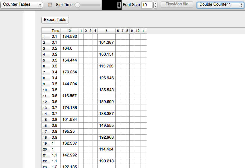
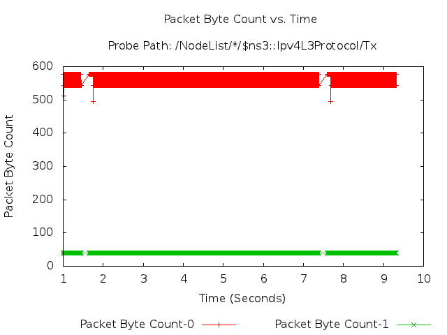
Once the test case execution ends it will create DlRlcStats.txt and UlRlcStats.txt. Key fields that need to be checked in statistics are:
|Start | end | Cell ID | IMSI | RNTI | LCID | TxBytes | RxBytes |
Test case executes in three epochs:
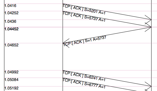
- In first Epoch (0.04s-1.04s) All UE’s and corresponding bearers gets attached and packet flow over the dedicated bearers activated.
- In second Epoch (1.04s-2.04s), bearer deactivation is instantiated, hence User can see relatively less number of TxBytes on UE_ID=1 and LCID=4 as compared to other bearers.
- In third Epoch (2.04s-3.04s) since bearer deactivation of UE_ID=1 and LCID=4 is completed, user will not see any logging related to LCID=4.
Test case passes if and only if
- IMSI=1 and LCID=4 completely removed in third epoch
- No packets seen in TxBytes and RxBytes corresponding to IMSI=1 and LCID=4
If above criteria do not match, the test case is considered to be failed
Adaptive Modulation and Coding Tests
The test suite lte-link-adaptation provides system tests recreating a
scenario with a single eNB and a single UE. Different test cases are created
corresponding to different SNR values perceived by the UE. The aim of the test
is to check that in each test case the chosen MCS corresponds to some known
reference values. These reference values are obtained by
re-implementing in Octave (see src/lte/test/reference/lte_amc.m) the
model described in Section Adaptive Modulation and Coding for the calculation of the
spectral efficiency, and determining the corresponding MCS index
by manually looking up the tables in [R1-081483]. The resulting test vector is
represented in Figure Test vector for Adaptive Modulation and Coding.
The MCS which is used by the simulator is measured by
obtaining the tracing output produced by the scheduler after 4ms (this
is needed to account for the initial delay in CQI reporting). The SINR
which is calcualted by the simulator is also obtained using the
LteChunkProcessor interface. The test
passes if both the following conditions are satisfied:
- the SINR calculated by the simulator correspond to the SNR
of the test vector within an absolute tolerance of
 ;
;
- the MCS index used by the simulator exactly corresponds to
the one in the test vector.
UE Measurements Tests
The test suite lte-ue-measurements provides system tests recreating an
inter-cell interference scenario identical of the one defined for
lte-interference test-suite. However, in this test the quantities to be
tested are represented by RSRP and RSRQ measurements performed by the UE in two
different points of the stack: the source, which is UE PHY layer, and the
destination, that is the eNB RRC.
The test vectors are obtained by the use of a dedicated octave script (available
in src/lte/test/reference/lte-ue-measurements.m), which does the link budget
calculations (including interference) corresponding to the topology of each
test case, and outputs the resulting RSRP and RSRQ. The obtained values are then
used for checking the correctness of the UE Measurements at PHY layer. After
that, they have to be converted according to 3GPP formatting for the purpose of
checking their correctness at eNB RRC level.
UE measurement configuration tests
Besides the previously mentioned test suite, there are 3 other test suites for
testing UE measurements: lte-ue-measurements-piecewise-1,
lte-ue-measurements-piecewise-2, and lte-ue-measurements-handover. These
test suites are more focused on the reporting trigger procedure, i.e. the
correctness of the implementation of the event-based triggering criteria is
verified here.
In more specific, the tests verify the timing and the content of each
measurement reports received by eNodeB. Each test case is an stand-alone LTE
simulation and the test case will pass if measurement report(s) only occurs at
the prescribed time and shows the correct level of RSRP (RSRQ is not verified at
the moment).
Piecewise configuration
The piecewise configuration aims to test a particular UE measurements
configuration. The simulation script will setup the corresponding measurements
configuration to the UE, which will be active throughout the simulation.
Since the reference values are precalculated by hands, several assumptions are
made to simplify the simulation. Firstly, the channel is only affected by path
loss model (in this case, Friis model is used). Secondly, the ideal RRC protocol
is used, and layer 3 filtering is disabled. Finally, the UE moves in a
predefined motion pattern between 4 distinct spots, as depicted in Figure
UE movement trace throughout the simulation in piecewise configuration below. Therefore the fluctuation of the
measured RSRP can be determined more easily.
The motivation behind the “teleport” between the predefined spots is to
introduce drastic change of RSRP level, which will guarantee the triggering of
entering or leaving condition of the tested event. By performing drastic
changes, the test can be run within shorter amount of time.
Figure Measured RSRP trace of an example Event A1 test case in piecewise
configuration below shows the measured RSRP after
layer 1 filtering by the PHY layer during the simulation with a piecewise
configuration. Because layer 3 filtering is disabled, these are the exact values
used by the UE RRC instance to evaluate reporting trigger procedure. Notice that
the values are refreshed every 200 ms, which is the default filtering period of
PHY layer measurements report. The figure also shows the time when entering and
leaving conditions of an example instance of Event A1 (serving cell becomes
better than threshold) occur during the simulation.
Each reporting criterion is tested several times with different threshold/offset
parameters. Some test scenarios also take hysteresis and time-to-trigger into
account. Figure Measured RSRP trace of an example Event A1 with hysteresis test case in
piecewise configuration depicts the effect of
hysteresis in another example of Event A1 test.
Piecewise configuration is used in two test suites of UE measurements. The first
one is lte-ue-measurements-piecewise-1, henceforth Piecewise test #1, which
simulates 1 UE and 1 eNodeB. The other one is lte-ue-measurements-piecewise-2,
which has 1 UE and 2 eNodeBs in the simulation.
Piecewise test #1 is intended to test the event-based criteria which are not
dependent on the existence of a neighbouring cell. These criteria include Event
A1 and A2. The other events are also briefly tested to verify that they are
still working correctly (albeit not reporting anything) in the absence of any
neighbouring cell. Table UE measurements test scenarios using piecewise configuration #1 below lists the
scenarios tested in piecewise test #1.
UE measurements test scenarios using piecewise configuration #1
| Test # |
Reporting Criteria |
Threshold/Offset |
Hysteresis |
Time-to-Trigger |
|---|
| 1 |
Event A1 |
Low |
No |
No |
| 2 |
Event A1 |
Normal |
No |
No |
| 3 |
Event A1 |
Normal |
No |
Short |
| 4 |
Event A1 |
Normal |
No |
Long |
| 5 |
Event A1 |
Normal |
No |
Super |
| 6 |
Event A1 |
Normal |
Yes |
No |
| 7 |
Event A1 |
High |
No |
No |
| 8 |
Event A2 |
Low |
No |
No |
| 9 |
Event A2 |
Normal |
No |
No |
| 10 |
Event A2 |
Normal |
No |
Short |
| 11 |
Event A2 |
Normal |
No |
Long |
| 12 |
Event A2 |
Normal |
No |
Super |
| 13 |
Event A2 |
Normal |
Yes |
No |
| 14 |
Event A2 |
High |
No |
No |
| 15 |
Event A3 |
Zero |
No |
No |
| 16 |
Event A4 |
Normal |
No |
No |
| 17 |
Event A5 |
Normal-Normal |
No |
No |
Other events such as Event A3, A4, and A5 depend on measurements of neighbouring
cell, so they are more thoroughly tested in Piecewise test #2. The simulation
places the nodes on a straight line and instruct the UE to “jump” in a similar
manner as in Piecewise test #1. Handover is disabled in the simulation, so the
role of serving and neighbouring cells do not switch during the simulation.
Table UE measurements test scenarios using piecewise configuration #2 below lists the scenarios tested in
Piecewise test #2.
UE measurements test scenarios using piecewise configuration #2
| Test # |
Reporting Criteria |
Threshold/Offset |
Hysteresis |
Time-to-Trigger |
|---|
| 1 |
Event A1 |
Low |
No |
No |
| 2 |
Event A1 |
Normal |
No |
No |
| 3 |
Event A1 |
Normal |
Yes |
No |
| 4 |
Event A1 |
High |
No |
No |
| 5 |
Event A2 |
Low |
No |
No |
| 6 |
Event A2 |
Normal |
No |
No |
| 7 |
Event A2 |
Normal |
Yes |
No |
| 8 |
Event A2 |
High |
No |
No |
| 9 |
Event A3 |
Positive |
No |
No |
| 10 |
Event A3 |
Zero |
No |
No |
| 11 |
Event A3 |
Zero |
No |
Short |
| 12 |
Event A3 |
Zero |
No |
Super |
| 13 |
Event A3 |
Zero |
Yes |
No |
| 14 |
Event A3 |
Negative |
No |
No |
| 15 |
Event A4 |
Low |
No |
No |
| 16 |
Event A4 |
Normal |
No |
No |
| 17 |
Event A4 |
Normal |
No |
Short |
| 18 |
Event A4 |
Normal |
No |
Super |
| 19 |
Event A4 |
Normal |
Yes |
No |
| 20 |
Event A4 |
High |
No |
No |
| 21 |
Event A5 |
Low-Low |
No |
No |
| 22 |
Event A5 |
Low-Normal |
No |
No |
| 23 |
Event A5 |
Low-High |
No |
No |
| 24 |
Event A5 |
Normal-Low |
No |
No |
| 25 |
Event A5 |
Normal-Normal |
No |
No |
| 26 |
Event A5 |
Normal-Normal |
No |
Short |
| 27 |
Event A5 |
Normal-Normal |
No |
Super |
| 28 |
Event A5 |
Normal-Normal |
Yes |
No |
| 29 |
Event A5 |
Normal-High |
No |
No |
| 30 |
Event A5 |
High-Low |
No |
No |
| 31 |
Event A5 |
High-Normal |
No |
No |
| 32 |
Event A5 |
High-High |
No |
No |
One note about the tests with time-to-trigger, they are tested using 3 different
values of time-to-trigger: short (shorter than report interval), long
(shorter than the filter measurement period of 200 ms), and super (longer than
200 ms). The first two ensure that time-to-trigger evaluation always use the
latest measurement reports received from PHY layer. While the last one is
responsible for verifying time-to-trigger cancellation, for example when a
measurement report from PHY shows that the entering/leaving condition is no
longer true before the first trigger is fired.
Handover configuration
The purpose of the handover configuration is to verify whether UE measurement
configuration is updated properly after a succesful handover takes place. For
this purpose, the simulation will construct 2 eNodeBs with different UE
measurement configuration, and the UE will perform handover from one cell to
another. The UE will be located on a straight line between the 2 eNodeBs, and
the handover will be invoked manually. The duration of each simulation is
2 seconds (except the last test case) and the handover is triggered exactly at
halfway of simulation.
The lte-ue-measurements-handover test suite covers various types of
configuration differences. The first one is the difference in report interval,
e.g. the first eNodeB is configured with 480 ms report interval, while the
second eNodeB is configured with 240 ms report interval. Therefore, when the UE
performed handover to the second cell, the new report interval must take effect.
As in piecewise configuration, the timing and the content of each measurement
report received by the eNodeB will be verified.
Other types of differences covered by the test suite are differences in event
and differences in threshold/offset. Table UE measurements test scenarios using handover configuration below
lists the tested scenarios.
UE measurements test scenarios using handover configuration
| Test # |
Test Subject |
Initial Configuration |
Post-Handover Configuration |
|---|
| 1 |
Report interval |
480 ms |
240 ms |
| 2 |
Report interval |
120 ms |
640 ms |
| 3 |
Event |
Event A1 |
Event A2 |
| 4 |
Event |
Event A2 |
Event A1 |
| 5 |
Event |
Event A3 |
Event A4 |
| 6 |
Event |
Event A4 |
Event A3 |
| 7 |
Event |
Event A2 |
Event A3 |
| 8 |
Event |
Event A3 |
Event A2 |
| 9 |
Event |
Event A4 |
Event A5 |
| 10 |
Event |
Event A5 |
Event A4 |
| 11 |
Threshold/offset |
RSRP range 52 (Event A1) |
RSRP range 56 (Event A1) |
| 12 |
Threshold/offset |
RSRP range 52 (Event A2) |
RSRP range 56 (Event A2) |
| 13 |
Threshold/offset |
A3 offset -30 (Event A3) |
A3 offset +30 (Event A3) |
| 14 |
Threshold/offset |
RSRP range 52 (Event A4) |
RSRP range 56 (Event A4) |
| 15 |
Threshold/offset |
RSRP range 52-52 (Event A5) |
RSRP range 56-56 (Event A5) |
| 16 |
Time-to-trigger |
1024 ms |
100 ms |
| 17 |
Time-to-trigger |
1024 ms |
640 ms |
Proportional Fair scheduler performance
The test suite lte-pf-ff-mac-scheduler creates different test cases with
a single eNB, using the Proportional Fair (PF) scheduler, and several UEs, all
having the same Radio Bearer specification. The test cases are grouped in two
categories in order to evaluate the performance both in terms of the adaptation
to the channel condition and from a fairness perspective.
In the first category of test cases, the UEs are all placed at the
same distance from the eNB, and hence all placed in order to have the
same SINR. Different test cases are implemented by using a different
SINR value and a different number of UEs. The test consists on
checking that the obtained throughput performance matches with the
known reference throughput up to a given tolerance. The expected
behavior of the PF scheduler when all UEs have the same SNR is that
each UE should get an equal fraction of the throughput obtainable by a
single UE when using all the resources. We calculate the reference
throughput value by dividing the throughput achievable by a single UE
at the given SNR by the total number of UEs.
Let  be the TTI duration,
  the transmission
bandwidth configuration in number of RBs,
the transmission
bandwidth configuration in number of RBs,  the modulation and
coding scheme in use at the given SINR and
the modulation and
coding scheme in use at the given SINR and  be the
transport block size as defined in [TS36213]. The reference
throughput
be the
transport block size as defined in [TS36213]. The reference
throughput  in bit/s achieved by each UE is calculated as
The curves labeled “PF” in Figure fig-lenaThrTestCase1 represent the test values
calculated for the PF scheduler tests of the first category, that we just described.
The second category of tests aims at verifying the fairness of the PF
scheduler in a more realistic simulation scenario where the UEs have a
different SINR (constant for the whole simulation). In these conditions, the PF
scheduler will give to each user a share of the system bandwidth that is
proportional to the capacity achievable by a single user alone considered its
SINR. In detail, let  be the modulation and coding scheme being used by
each UE (which is a deterministic function of the SINR of the UE, and is hence
known in this scenario). Based on the MCS, we determine the achievable
rate
be the modulation and coding scheme being used by
each UE (which is a deterministic function of the SINR of the UE, and is hence
known in this scenario). Based on the MCS, we determine the achievable
rate  for each user
  using the
procedure described in Section~ref{sec:pfs}. We then define the
achievable rate ratio
using the
procedure described in Section~ref{sec:pfs}. We then define the
achievable rate ratio  of each user as
Let now  be the throughput actually achieved by the UE , which
is obtained as part of the simulation output. We define the obtained throughput
ratio
be the throughput actually achieved by the UE , which
is obtained as part of the simulation output. We define the obtained throughput
ratio  of UE as
The test consists of checking that the following condition is verified:
if so, it means that the throughput obtained by each UE over the whole
simulation matches with the steady-state throughput expected by the PF scheduler
according to the theory. This test can be derived from [Holtzman2000]
as follows. From Section 3 of [Holtzman2000], we know that
where  is a constant. By substituting the above into the
definition of given previously, we get
is a constant. By substituting the above into the
definition of given previously, we get
which is exactly the expression being used in the test.
Figure Throughput ratio evaluation for the PF scheduler in a scenario
where the UEs have MCS index presents the results obtained in a test case with
UEs  that are located at a distance from the base
station such that they will use respectively the MCS index
that are located at a distance from the base
station such that they will use respectively the MCS index  . From the figure, we note that, as expected, the obtained throughput is
proportional to the achievable rate. In other words, the PF scheduler assign
more resources to the users that use a higher MCS index.
. From the figure, we note that, as expected, the obtained throughput is
proportional to the achievable rate. In other words, the PF scheduler assign
more resources to the users that use a higher MCS index.
Blind Average Throughput scheduler performance
Test suites lte-tdbet-ff-mac-scheduler and lte-fdbet-ff-mac-scheduler create different
test cases with a single eNB and several UEs, all having the same Radio Bearer specification.
In the first test case of lte-tdbet-ff-mac-scheduler and lte-fdbet-ff-mac-scheduler,
the UEs are all placed at the same distance from the eNB, and hence all placed in order to
have the same SNR. Different test cases are implemented by using a different SNR value and
a different number of UEs. The test consists on checking that the obtained throughput performance
matches with the known reference throughput up to a given tolerance. In long term, the expected
behavior of both TD-BET and FD-BET when all UEs have the same SNR is that each UE should get an
equal throughput. However, the exact throughput value of TD-BET and FD-BET in this test case is not
the same.
When all UEs have the same SNR, TD-BET can be seen as a specific case of PF where achievable rate equals
to 1. Therefore, the throughput obtained by TD-BET is equal to that of PF. On the other hand, FD-BET performs
very similar to the round robin (RR) scheduler in case of that all UEs have the same SNR and the number of UE( or RBG)
is an integer multiple of the number of RBG( or UE). In this case, FD-BET always allocate the same number of RBGs
to each UE. For example, if eNB has 12 RBGs and there are 6 UEs, then each UE will get 2 RBGs in each TTI.
Or if eNB has 12 RBGs and there are 24 UEs, then each UE will get 2 RBGs per two TTIs. When the number of
UE (RBG) is not an integer multiple of the number of RBG (UE), FD-BET will not follow the RR behavior because
it will assigned different number of RBGs to some UEs, while the throughput of each UE is still the same.
The second category of tests aims at verifying the fairness of the both TD-BET and FD-BET schedulers in a more realistic
simulation scenario where the UEs have a different SNR (constant for the whole simulation). In this case,
both scheduler should give the same amount of averaged throughput to each user.
Specifically, for TD-BET, let  be the fraction of time allocated to user i in total simulation time,
 be the the full bandwidth achievable rate for user i and be the achieved throughput of
user i. Then we have:
be the the full bandwidth achievable rate for user i and be the achieved throughput of
user i. Then we have:
In TD-BET, the sum of for all user equals one. In long term, all UE has the same so that we replace
by . Then we have:
Token Band Fair Queue scheduler performance
Test suites lte-fdtbfq-ff-mac-scheduler and lte-tdtbfq-ff-mac-scheduler create different
test cases for testing three key features of TBFQ scheduler: traffic policing, fairness and traffic
balance. Constant Bit Rate UDP traffic is used in both downlink and uplink in all test cases.
The packet interval is set to 1ms to keep the RLC buffer non-empty. Different traffic rate is
achieved by setting different packet size. Specifically, two classes of flows are created in the
testsuites:
- Homogeneous flow: flows with the same token generation rate and packet arrival rate
- Heterogeneous flow: flows with different packet arrival rate, but with the same token generation rate
In test case 1 verifies traffic policing and fairness features for the scenario that all UEs are
placed at the same distance from the eNB. In this case, all Ues have the same SNR value. Different
test cases are implemented by using a different SNR value and a different number of UEs. Because each
flow have the same traffic rate and token generation rate, TBFQ scheduler will guarantee the same
throughput among UEs without the constraint of token generation rate. In addition, the exact value
of UE throughput is depended on the total traffic rate:
- If total traffic rate <= maximum throughput, UE throughput = traffic rate
- If total traffic rate > maximum throughput, UE throughput = maximum throughput / N
Here, N is the number of UE connected to eNodeB. The maximum throughput in this case equals to the rate
that all RBGs are assigned to one UE(e.g., when distance equals 0, maximum throughput is 2196000 byte/sec).
When the traffic rate is smaller than max bandwidth, TBFQ can police the traffic by token generation rate
so that the UE throughput equals its actual traffic rate (token generation rate is set to traffic
generation rate); On the other hand, when total traffic rate is bigger than the max throughput, eNodeB
cannot forward all traffic to UEs. Therefore, in each TTI, TBFQ will allocate all RBGs to one UE due to
the large packets buffered in RLC buffer. When a UE is scheduled in current TTI, its token counter is decreased
so that it will not be scheduled in the next TTI. Because each UE has the same traffic generation rate,
TBFQ will serve each UE in turn and only serve one UE in each TTI (both in TD TBFQ and FD TBFQ).
Therefore, the UE throughput in the second condition equals to the evenly share of maximum throughput.
Test case 2 verifies traffic policing and fairness features for the scenario that each UE is placed at
the different distance from the eNB. In this case, each UE has the different SNR value. Similar to test
case 1, UE throughput in test case 2 is also depended on the total traffic rate but with a different
maximum throughput. Suppose all UEs have a high traffic load. Then the traffic will saturate the RLC buffer
in eNodeB. In each TTI, after selecting one UE with highest metric, TBFQ will allocate all RBGs to this
UE due to the large RLC buffer size. On the other hand, once RLC buffer is saturated, the total throughput
of all UEs cannot increase any more. In addition, as we discussed in test case 1, for homogeneous flows
which have the same t_i and r_i, each UE will achieve the same throughput in long term. Therefore, we
can use the same method in TD BET to calculate the maximum throughput:

Here, is the maximum throughput. be the the full bandwidth achievable rate
for user i.  is the number of UE.
When the totol traffic rate is bigger than , the UE throughput equals to  . Otherwise, UE throughput
equals to its traffic generation rate.
. Otherwise, UE throughput
equals to its traffic generation rate.
In test case 3, three flows with different traffic rate are created. Token generation rate for each
flow is the same and equals to the average traffic rate of three flows. Because TBFQ use a shared token
bank, tokens contributed by UE with lower traffic load can be utilized by UE with higher traffic load.
In this way, TBFQ can guarantee the traffic rate for each flow. Although we use heterogeneous flow here,
the calculation of maximum throughput is as same as that in test case 2. In calculation max throughput
of test case 2, we assume that all UEs suffer high traffic load so that scheduler always assign all RBGs
to one UE in each TTI. This assumes is also true in heterogeneous flow case. In other words, whether
those flows have the same traffic rate and token generation rate, if their traffic rate is bigger enough,
TBFQ performs as same as it in test case 2. Therefore, the maximum bandwidth in test case 3 is as
same as it in test case 2.
In test case 3, in some flows, token generate rate does not equal to MBR, although all flows are CBR
traffic. This is not accorded with our parameter setting rules. Actually, the traffic balance feature
is used in VBR traffic. Because different UE’s peak rate may occur in different time, TBFQ use shared
token bank to balance the traffic among those VBR traffics. Test case 3 use CBR traffic to verify this
feature. But in the real simulation, it is recommended to set token generation rate to MBR.
Building Propagation Loss Model
The aim of the system test is to verify the integration of the
BuildingPathlossModel with the lte module. The test exploits a set of
three pre calculated losses for generating the expected SINR at the
receiver counting the transmission and the noise powers. These SINR
values are compared with the results obtained from a LTE
simulation that uses the BuildingPathlossModel. The reference loss values are
calculated off-line with an Octave script
(/test/reference/lte_pathloss.m). Each test case passes if the
reference loss value is equal to the value calculated by the simulator
within a tolerance of  dB, which accouns for numerical
errors in the calculations.
dB, which accouns for numerical
errors in the calculations.
Physical Error Model
The test suite lte-phy-error-model generates different test cases for
evaluating both data and control error models. For what concern the data, the
test consists of six test cases with single eNB and a various number of UEs,
all having the same Radio Bearer specification. Each test is designed for
evaluating the error rate perceived by a specific TB size in order to verify
that it corresponds to the expected values according to the BLER generated for
CB size analog to the TB size. This means that, for instance, the test will
check that the performance of a TB of bits is analogous to the one of
a CB size of bits by collecting the performance of a user which has
been forced the generation of a such TB size according to the distance to eNB.
In order to significantly test the BLER at MAC level, we configured the Adaptive
Modulation and Coding (AMC) module, the LteAmc class, for making it less
robust to channel conditions by using the PiroEW2010 AMC model and configuring
it to select the MCS considering a target BER of 0.03 (instead of the default
value of 0.00005). We note that these values do not reflect the actual BER,
since they come from an analytical bound which does not consider all the
transmission chain aspects; therefore the BER and BLER actually experienced at
the reception of a TB is in general different.
The parameters of the six test cases are reported in the following:
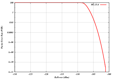
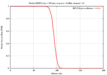
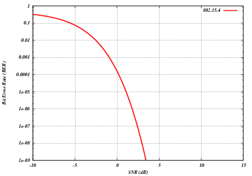
- 4 UEs placed 1800 meters far from the eNB, which implies the use of MCS 2
(SINR of -5.51 dB) and a TB of 256 bits, that in turns produce a BLER of 0.33
(see point A in figure BLER for tests 1, 2, 3.).
- 2 UEs placed 1800 meters far from the eNB, which implies the use of MCS 2
(SINR of -5.51 dB) and a TB of 528 bits, that in turns produce a BLER of 0.11
(see point B in figure BLER for tests 1, 2, 3.).
- 1 UE placed 1800 meters far from the eNB, which implies the use of MCS 2
(SINR of -5.51 dB) and a TB of 1088 bits, that in turns produce a BLER of
0.02 (see point C in figure BLER for tests 1, 2, 3.).
- 1 UE placed 600 meters far from the eNB, which implies the use of MCS 12
(SINR of 4.43 dB) and a TB of 4800 bits, that in turns produce a BLER of 0.3
(see point D in figure BLER for tests 4, 5.).
- 3 UEs placed 600 meters far from the eNB, which implies the use of MCS 12
(SINR of 4.43 dB) and a TB of 1632 bits, that in turns produce a BLER of 0.55
(see point E in figure BLER for tests 4, 5.).
- 1 UE placed 470 meters far from the eNB, which implies the use of MCS 16
(SINR of 8.48 dB) and a TB of 7272 bits (segmented in 2 CBs of 3648 and 3584
bits), that in turns produce a BLER of 0.14, since each CB has CBLER equal to
0.075 (see point F in figure BLER for test 6.).
The test condition verifies that in each test case the expected number of
packets received correctly corresponds to a Bernoulli distribution with a
confidence interval of 99%, where the probability of success in each trail is
 and
and  is the total number of packets sent.
The error model of PCFICH-PDCCH channels consists of 4 test cases with a single
UE and several eNBs, where the UE is connected to only one eNB in order to have
the remaining acting as interfering ones. The errors on data are disabled in
order to verify only the ones due to erroneous decodification of PCFICH-PDCCH.
As before, the system has been forced on working in a less conservative fashion
in the AMC module for appreciating the results in border situations. The
parameters of the 4 tests cases are reported in the following:
- 2 eNBs placed 1078 meters far from the UE, which implies a SINR of -2.00 dB
and a TB of 217 bits, that in turns produce a BLER of 0.007.
- 3 eNBs placed 1040 meters far from the UE, which implies a SINR of -4.00 dB
and a TB of 217 bits, that in turns produce a BLER of 0.045.
- 4 eNBs placed 1250 meters far from the UE, which implies a SINR of -6.00 dB
and a TB of 133 bits, that in turns produce a BLER of 0.206.
- 5 eNBs placed 1260 meters far from the UE, which implies a SINR of -7.00 dB
and a TB of 81 bits, that in turns produce a BLER of 0.343.
The test condition verifies that in each test case the expected number
of packets received correct corresponds to a Bernoulli distribution
with a confidence interval of 99.8%, where the probability of success
in each trail is and is the total number of
packet sent. The larger confidence interval is due to the errors that
might be produced in quantizing the MI and the error curve.
HARQ Model
The test suite lte-harq includes two tests for evaluating the HARQ model and the related extension in the error model. The test consists on checking whether the amount of bytes received during the simulation corresponds to the expected ones according to the values of transport block and the HARQ dynamics. In detail, the test checks whether the throughput obtained after one HARQ retransmission is the expeted one. For evaluating the expected throughput the expected TB delivering time has been evaluated according to the following formula:
where  is the probability of receiving with success the HARQ block at the attempt (i.e., the RV with 3GPP naming). According to the scenarios, in the test we always have
  equal to 0.0, while
  varies in the two tests, in detail:
The expected throughput is calculted by counting the number of transmission slots available during the simulation (e.g., the number of TTIs) and the size of the TB in the simulation, in detail:
where  is the total number of TTIs in 1 second.
The test is performed both for Round Robin scheduler. The test passes if the measured throughput matches with the reference throughput within a relative tolerance of 0.1. This tolerance is needed to account for the transient behavior at the beginning of the simulation and the on-fly blocks at the end of the simulation.
is the total number of TTIs in 1 second.
The test is performed both for Round Robin scheduler. The test passes if the measured throughput matches with the reference throughput within a relative tolerance of 0.1. This tolerance is needed to account for the transient behavior at the beginning of the simulation and the on-fly blocks at the end of the simulation.
MIMO Model
The test suite lte-mimo aims at verifying both the effect of the gain considered for each Transmission Mode on the system performance and the Transmission Mode switching through the scheduler interface. The test consists on checking whether the amount of bytes received during a certain window of time (0.1 seconds in our case) corresponds to the expected ones according to the values of transport block
size reported in table 7.1.7.2.1-1 of [TS36213], similarly to what done for the tests of the schedulers.
The test is performed both for Round Robin and Proportional Fair schedulers. The test passes if the measured throughput matches with the reference throughput within a relative tolerance of 0.1. This tolerance is needed to account for the
transient behavior at the beginning of the simulation and the transition phase between the Transmission Modes.
Antenna Model integration
The test suite lte-antenna checks that the AntennaModel integrated
with the LTE model works correctly. This test suite recreates a
simulation scenario with one eNB node at coordinates (0,0,0) and one
UE node at coordinates (x,y,0). The eNB node is configured with an
CosineAntennaModel having given orientation and beamwidth. The UE
instead uses the default IsotropicAntennaModel. The test
checks that the received power both in uplink and downlink account for
the correct value of the antenna gain, which is determined
offline; this is implemented by comparing the uplink and downlink SINR
and checking that both match with the reference value up to a
tolerance of  which accounts for numerical errors.
Different test cases are provided by varying the x and y coordinates
of the UE, and the beamwidth and the orientation of the antenna of
the eNB.
which accounts for numerical errors.
Different test cases are provided by varying the x and y coordinates
of the UE, and the beamwidth and the orientation of the antenna of
the eNB.
RLC
Two test suites lte-rlc-um-transmitter and
lte-rlc-am-transmitter check that the UM RLC and the AM RLC
implementation work correctly. Both these suites work by testing RLC
instances connected to special test entities that play the role of the
MAC and of the PDCP, implementing respectively the LteMacSapProvider
and LteRlcSapUser interfaces. Different test cases (i.e., input test
vector consisting of series of primitive calls by the MAC and the
PDCP) are provided that check the behavior in the following cases:
- one SDU, one PDU: the MAC notifies a TX opportunity causes the creation of a PDU which exactly
contains a whole SDU
- segmentation: the MAC notifies multiple TX opportunities that are smaller than the SDU
size stored in the transmission buffer, which is then to be fragmented and hence
multiple PDUs are generated;
- concatenation: the MAC notifies a TX opportunity that is bigger than the SDU, hence
multiple SDUs are concatenated in the same PDU
- buffer status report: a series of new SDUs notifications by the
PDCP is inteleaved with a series of TX opportunity notification in
order to verify that the buffer status report procedure is
correct.
In all these cases, an output test vector is determine manually from
knowledge of the input test vector and knowledge of the expected
behavior. These test vector are specialized for UM RLC and
AM RLC due to their different behavior. Each test case passes if the
sequence of primitives triggered by the RLC instance being tested is
exacly equal to the output test vector. In particular, for each PDU
transmitted by the RLC instance, both the size and the content of the
PDU are verified to check for an exact match with the test vector.
The AM RLC implementation features an additional test suite,
lte-rlc-am-e2e, which test the correct retransmission of RLC PDUs
in presence of channel losses. The test instantiates an RLC AM
transmitter and a receiver, and interposes a channel that randomly
drops packet according to a fixed loss probability. Different test
cases are instantiated using different RngRun values and different
loss probability values. Each test case passes if at the end of the
simulation all SDUs are correctly delivered to the upper layers of the
receiving RLC AM entity.
RRC
The test suite lte-rrc tests the correct functionality of the following aspects:
- MAC Random Access
- RRC System Information Acquisition
- RRC Connection Establishment
- RRC Reconfiguration
The test suite considers a type of scenario with four eNBs aligned in a square
layout with 100-meter edges. Multiple UEs are located at a specific spot on the
diagonal of the square and are instructed to connect to the first eNB. Each test
case implements an instance of this scenario with specific values of the
following parameters:
- number of UEs
- number of Data Radio Bearers to be activated for each UE
- time
 at which the first UE is instructed to start connecting to the eNB
- time interval
 between the start of connection of UE and UE
  ; the time at which user connects is thus determined as
  sdf
sdf
- the relative position of the UEs on the diagonal of the square, where higher
values indicate larger distance from the serving eNodeB, i.e., higher
interference from the other eNodeBs
- a boolean flag indicating whether the ideal or the real RRC protocol model is used
Each test cases passes if a number of test conditions are positively evaluated for each UE after a delay  from the time it started connecting to the eNB. The delay is determined as
where:
 is the max delay necessary for the acquisition of System Information. We set it to 90ms accounting for 10ms for the MIB acquisition and 80ms for the subsequent SIB2 acquisition
 is the delay for the MAC Random Access (RA)
procedure. This depends on preamble collisions as well as on the
availability of resources for the UL grant allocation. The total amount of
necessary RA attempts depends on preamble collisions and failures
to allocate the UL grant because of lack of resources. The number
of collisions depends on the number of UEs that try to access
simultaneously; we estimated that for a
is the delay for the MAC Random Access (RA)
procedure. This depends on preamble collisions as well as on the
availability of resources for the UL grant allocation. The total amount of
necessary RA attempts depends on preamble collisions and failures
to allocate the UL grant because of lack of resources. The number
of collisions depends on the number of UEs that try to access
simultaneously; we estimated that for a  RA success
probability, 5 attempts are sufficient for up to 20 UEs, and 10 attempts for up
to 50 UEs.
For the UL grant, considered the system bandwidth and the
default MCS used for the UL grant (MCS 0), at most 4 UL grants can
be assigned in a TTI; so for UEs trying to
do RA simultaneously the max number of attempts due to the UL grant
issue is
RA success
probability, 5 attempts are sufficient for up to 20 UEs, and 10 attempts for up
to 50 UEs.
For the UL grant, considered the system bandwidth and the
default MCS used for the UL grant (MCS 0), at most 4 UL grants can
be assigned in a TTI; so for UEs trying to
do RA simultaneously the max number of attempts due to the UL grant
issue is  . The time for
a RA attempt is determined by 3ms + the value of
LteEnbMac::RaResponseWindowSize, which defaults to 3ms, plus 1ms
for the scheduling of the new transmission.
. The time for
a RA attempt is determined by 3ms + the value of
LteEnbMac::RaResponseWindowSize, which defaults to 3ms, plus 1ms
for the scheduling of the new transmission. is the delay required for the transmission of RRC CONNECTION
SETUP + RRC CONNECTION SETUP COMPLETED. We consider a round trip
delay of 10ms plus
is the delay required for the transmission of RRC CONNECTION
SETUP + RRC CONNECTION SETUP COMPLETED. We consider a round trip
delay of 10ms plus  considering that 2
RRC packets have to be transmitted and that at most 4 such packets
can be transmitted per TTI. In cases where interference is high, we
accommodate one retry attempt by the UE, so we double the
value and then add on top of it (because the timeout has
reset the previously received SIB2).
considering that 2
RRC packets have to be transmitted and that at most 4 such packets
can be transmitted per TTI. In cases where interference is high, we
accommodate one retry attempt by the UE, so we double the
value and then add on top of it (because the timeout has
reset the previously received SIB2). is the delay required for eventually needed RRC
CONNECTION RECONFIGURATION transactions. The number of transactions needed is
1 for each bearer activation. Similarly to what done for
, for each transaction we consider a round trip
delay of 10ms plus .
delay of 20ms.
is the delay required for eventually needed RRC
CONNECTION RECONFIGURATION transactions. The number of transactions needed is
1 for each bearer activation. Similarly to what done for
, for each transaction we consider a round trip
delay of 10ms plus .
delay of 20ms.
The base version of the test LteRrcConnectionEstablishmentTestCase
tests for correct RRC connection establishment in absence of channel
errors. The conditions that are evaluated for this test case to pass
are, for each UE:
- the RRC state at the UE is CONNECTED_NORMALLY
- the UE is configured with the CellId, DlBandwidth, UlBandwidth,
DlEarfcn and UlEarfcn of the eNB
- the IMSI of the UE stored at the eNB is correct
- the number of active Data Radio Bearers is the expected one, both
at the eNB and at the UE
- for each Data Radio Bearer, the following identifiers match between
the UE and the eNB: EPS bearer id, DRB id, LCID
The test variant LteRrcConnectionEstablishmentErrorTestCase is
similar except for the presence of errors in the transmission of a
particular RRC message of choice during the first connection
attempt. The error is obtained by temporarily moving the UE to a far
away location; the time of movement has been determined empyrically
for each instance of the test case based on the message that it was
desidred to be in error. the test case checks that at least one of the following
conditions is false at the time right before the UE is moved back to
the original location:
- the RRC state at the UE is CONNECTED_NORMALLY
- the UE context at the eNB is present
- the RRC state of the UE Context at the eNB is CONNECTED_NORMALLY
Additionally, all the conditions of the
LteRrcConnectionEstablishmentTestCase are evaluated - they are
espected to be true because of the NAS behavior of immediately
re-attempting the connection establishment if it fails.
Initial cell selection
The test suite lte-cell-selection is responsible for verifying the
Initial Cell Selection procedure. The test is a simulation of a small
network of 2 non-CSG cells and 2 non-CSG cells. Several static UEs are then
placed at predefined locations. The UEs enter the simulation without being
attached to any cell. Initial cell selection is enabled for these UEs, so each
UE will find the best cell and attach to it by themselves.
At predefined check points time during the simulation, the test verifies that
every UE is attached to the right cell. Moreover, the test also ensures that the
UE is properly connected, i.e., its final state is CONNECTED_NORMALLY. Figure
Sample result of cell selection test depicts the network layout and the
expected result. When a UE is depicted as having 2 successful cell selections
(e.g., UE #3 and #4), any of them is accepted by the test case.
The figure shows that CSG members may attach to either CSG or non-CSG cells, and
simply choose the stronger one. On the other hand, non-members can only attach
to non-CSG cells, even when they are actually receiving stronger signal from a
CSG cell.
For reference purpose, Table UE error rate in Initial Cell Selection test shows the
error rate of each UE when receiving transmission from the control channel.
Based on this information, the check point time for UE #3 is done at a later
time than the others to compensate for its higher risk of failure.
UE error rate in Initial Cell Selection test
| UE # |
Error rate |
|---|
| 1 |
0.00% |
| 2 |
1.44% |
| 3 |
12.39% |
| 4 |
0.33% |
| 5 |
0.00% |
| 6 |
0.00% |
The test uses the default Friis path loss model and without any channel fading
model.
GTP-U protocol
The unit test suite epc-gtpu checks that the encoding and decoding of the GTP-U
header is done correctly. The test fills in a header with a set of
known values, adds the header to a packet, and then removes the header
from the packet. The test fails if, upon removing, any of the fields
in the GTP-U header is not decoded correctly. This is detected by
comparing the decoded value from the known value.
S1-U interface
Two test suites (epc-s1u-uplink and epc-s1u-downlink) make
sure that the S1-U interface implementation works correctly in
isolation. This is achieved by creating a set of simulation scenarios
where the EPC model alone is used, without the LTE model (i.e.,
without the LTE radio protocol stack, which is replaced by simple CSMA
devices). This checks that the
interoperation between multiple EpcEnbApplication instances in
multiple eNBs and the EpcSgwPgwApplication instance in the SGW/PGW
node works correctly in a variety of scenarios, with varying numbers
of end users (nodes with a CSMA device installed), eNBs, and different
traffic patterns (packet sizes and number of total packets).
Each test case works by injecting the chosen traffic pattern in the
network (at the considered UE or at the remote host for in the uplink or the
downlink test suite respectively) and checking that at the receiver
(the remote host or each considered UE, respectively) that exactly the same
traffic patterns is received. If any mismatch in the transmitted and
received traffic pattern is detected for any UE, the test fails.
TFT classifier
The test suite epc-tft-classifier checks in isolation that the
behavior of the EpcTftClassifier class is correct. This is performed
by creating different classifier instances where different TFT
instances are activated, and testing for each classifier that an
heterogeneous set of packets (including IP and TCP/UDP headers) is
classified correctly. Several test cases are provided that check the
different matching aspects of a TFT (e.g. local/remote IP address, local/remote port) both for uplink and
downlink traffic. Each test case corresponds to a specific packet and
a specific classifier instance with a given set of TFTs. The test case
passes if the bearer identifier returned by the classifier exactly
matches with the one that is expected for the considered packet.
End-to-end LTE-EPC data plane functionality
The test suite lte-epc-e2e-data ensures the correct end-to-end
functionality of the LTE-EPC data plane. For each test case in this
suite, a complete LTE-EPC simulation
scenario is created with the following characteristics:
- a given number of eNBs
- for each eNB, a given number of UEs
- for each UE, a given number of active EPS bearers
- for each active EPS bearer, a given traffic pattern (number of UDP
packets to be transmitted and packet size)
Each test is executed by transmitting the given traffic pattern both
in the uplink and in the downlink, at subsequent time intervals. The
test passes if all the following conditions are satisfied:
- for each active EPS bearer, the transmitted and received traffic
pattern (respectively at the UE and the remote host for uplink,
and vice versa for downlink) is exactly the same
- for each active EPS bearer and each direction (uplink or downlink),
exactly the expected number of packet flows over the corresponding
RadioBearer instance
X2 handover
The test suite lte-x2-handover checks the correct functionality of the X2 handover procedure. The scenario being tested is a topology with two eNBs connected by an X2 interface. Each test case is a particular instance of this scenario defined by the following parameters:
- the number of UEs that are initially attached to the first eNB
- the number of EPS bearers activated for each UE
- a list of handover events to be triggered, where each event is defined by:
+ the start time of the handover trigger
+ the index of the UE doing the handover
+ the index of the source eNB
+ the index of the target eNB
- a boolean flag indicating whether the target eNB admits the handover or not
- a boolean flag indicating whether the ideal RRC protocol is to be used instead of the real RRC protocol
- the type of scheduler to be used (RR or PF)
Each test case passes if the following conditions are true:
- at time 0.06s, the test CheckConnected verifies that each UE is connected to the first eNB
- for each event in the handover list:
- at the indicated event start time, the indicated UE is connected to the indicated source eNB
- 0.1s after the start time, the indicated UE is connected to the indicated target eNB
- 0.6s after the start time, for each active EPS bearer, the uplink and downlink sink applications of the indicated UE have achieved a number of bytes which is at least half the number of bytes transmitted by the corresponding source applications
The condition “UE is connected to eNB” is evaluated positively if and only if all the following conditions are met:
- the eNB has the context of the UE (identified by the RNTI value
retrieved from the UE RRC)
- the RRC state of the UE at the eNB is CONNECTED_NORMALLY
- the RRC state at the UE is CONNECTED_NORMALLY
- the UE is configured with the CellId, DlBandwidth, UlBandwidth,
DlEarfcn and UlEarfcn of the eNB
- the IMSI of the UE stored at the eNB is correct
- the number of active Data Radio Bearers is the expected one, both
at the eNB and at the UE
- for each Data Radio Bearer, the following identifiers match between
the UE and the eNB: EPS bearer id, DRB id, LCID
Automatic X2 handover
The test suite lte-x2-handover-measures checks the correct functionality of the handover
algorithm. The scenario being tested is a topology with two, three or four eNBs connected by
an X2 interface. The eNBs are located in a straight line in the X-axes. A UE moves along the
X-axes going from the neighbourhood of one eNB to the next eNB. Each test case is a particular
instance of this scenario defined by the following parameters:
- the number of eNBs in the X-axes
- the number of UEs
- the number of EPS bearers activated for the UE
- a list of check point events to be triggered, where each event is defined by:
+ the time of the first check point event
+ the time of the last check point event
+ interval time between two check point events
+ the index of the UE doing the handover
+ the index of the eNB where the UE must be connected
- a boolean flag indicating whether UDP traffic is to be used instead of TCP traffic
- the type of scheduler to be used
- the type of handover algorithm to be used
- a boolean flag indicating whether handover is admitted by default
- a boolean flag indicating whether the ideal RRC protocol is to be used instead of the
real RRC protocol
The test suite consists of many test cases. In fact, it has been one of the most
time-consuming test suite in ns-3. The test cases run with some combination of
the following variable parameters:
Each test case passes if the following conditions are true:
- at time 0.08s, the test CheckConnected verifies that each UE is connected to the first eNB
- for each event in the check point list:
- at the indicated check point time, the indicated UE is connected to the indicated eNB
- 0.5s after the check point, for each active EPS bearer, the uplink and downlink sink
applications of the UE have achieved a number of bytes which is at least half the number
of bytes transmitted by the corresponding source applications
The condition “UE is connected to eNB” is evaluated positively if and only if all the following conditions are met:
- the eNB has the context of the UE (identified by the RNTI value
retrieved from the UE RRC)
- the RRC state of the UE at the eNB is CONNECTED_NORMALLY
- the RRC state at the UE is CONNECTED_NORMALLY
- the UE is configured with the CellId, DlBandwidth, UlBandwidth,
DlEarfcn and UlEarfcn of the eNB
- the IMSI of the UE stored at the eNB is correct
- the number of active Data Radio Bearers is the expected one, both
at the eNB and at the UE
- for each Data Radio Bearer, the following identifiers match between
the UE and the eNB: EPS bearer id, DRB id, LCID
Handover delays
Handover procedure consists of several message exchanges between UE, source
eNodeB, and target eNodeB over both RRC protocol and X2 interface. Test suite
lte-handover-delay verifies that this procedure consistently spends the
same amount of time.
The test suite will run several handover test cases. Eact test case is an
individual simulation featuring a handover at a specified time in simulation.
For example, the handover in the first test case is invoked at time +0.100s,
while in the second test case it is at +0.101s. There are 10 test cases, each
testing a different subframe in LTE. Thus the last test case has the handover
at +0.109s.
The simulation scenario in the test cases is as follow:
- EPC is enabled
- 2 eNodeBs with circular (isotropic) antenna, separated by 1000 meters
- 1 static UE positioned exactly in the center between the eNodeBs
- no application installed
- no channel fading
- default path loss model (Friis)
- 0.300s simulation duration
The test case runs as follow. At the beginning of the simulation, the UE is
attached to the first eNodeB. Then at the time specified by the test case input
argument, a handover request will be explicitly issued to the second eNodeB.
The test case will then record the starting time, wait until the handover is
completed, and then record the completion time. If the difference between the
completion time and starting time is less than a predefined threshold, then the
test passes.
A typical handover in the current ns-3 implementation takes 4.2141 ms when using
Ideal RRC protocol model, and 19.9283 ms when using Real RRC protocol model.
Accordingly, the test cases use 5 ms and 20 ms as the maximum threshold values.
The test suite runs 10 test cases with Ideal RRC protocol model and 10 test
cases with Real RRC protocol model. More information regarding these models can
be found in Section RRC protocol models.
The motivation behind using subframes as the main test parameters is the fact
that subframe index is one of the factors for calculating RA-RNTI, which is used
by Random Access during the handover procedure. The test cases verify this
computation, utilizing the fact that the handover will be delayed when this
computation is broken. In the default simulation configuration, the handover
delay observed because of a broken RA-RNTI computation is typically 6 ms.
Selection of target cell in handover algorithm
eNodeB may utilize Handover algorithm to automatically create
handover decisions during simulation. The decision includes the UE which should
do the handover and the target cell where the UE should perform handover to.
The test suite lte-handover-target verifies that the handover algorithm is
making the right decision, in particular, in choosing the right target cell. It
consists of several short test cases for different network topology (2×2 grid
and 3×2 grid) and types of handover algorithm (the A2-A4-RSRQ handover algorithm
and the strongest cell handover algorithm).
Each test case is a simulation of a micro-cell environment with the following
parameter:
- EPC is enabled
- several circular (isotropic antenna) micro-cell eNodeBs in a rectangular grid
layout, with 130 m distance between each adjacent point
- 1 static UE, positioned close to and attached to the source cell
- no control channel error model
- no application installed
- no channel fading
- default path loss model (Friis)
- 1s simulation duration
To trigger a handover, the test case “shutdowns” the source cell at +0.5s
simulation time. Figure lte-handover-target test scenario in a 2×2 grid below
illustrates the process. This is done by setting the source cell’s Tx power to
a very low value. As a result, the handover algorithm notices that the UE
deserves a handover and several neighbouring cells become candidates of target
cell at the same time.
The test case then verifies that the handover algorithm, when faced with more
than one options of target cells, is able to choose the right one.
Downlink Power Control
The test suite lte-downlink-power-control checks correctness of Downlink
Power Control in three different ways:
- LteDownlinkPowerControlSpectrumValue test case check if
LteSpectrumValueHelper::CreateTxPowerSpectralDensity is creating correct
spectrum value for PSD for downlink transmission. The test vector contain EARFCN,
system bandwidth, TX power, TX power for each RB, active RBs, and expected TxPSD.
The test passes if TxPDS generated by
LteSpectrumValueHelper::CreateTxPowerSpectralDensity is equal to expected TxPSD.
- LteDownlinkPowerControlTestCase test case check if TX power difference between
data and control channel is equal to configured PdschConfigDedicated::P_A value.
TX power of control channel is measured by LteTestSinrChunkProcessor added
to RsPowerChunkProcessor list in UE DownlinkSpectrumPhy. Tx power of data
channel is measured in similar way, but it had to be implemented. Now
LteTestSinrChunkProcessor is added to DataPowerChunkProcessor list in UE
DownlinkSpectrumPhy. Test vector contain a set of all avaiable P_A values. Test
pass if power diffrence equals P_A value.
- LteDownlinkPowerControlRrcConnectionReconfiguration test case check if
RrcConnectionReconfiguration is performed correctly. When FR entity gets UE
measurements, it immediately calls function to change P_A value for this UE and also
triggers callback connected with this event. Then, test check if UE gets
RrcConnectionReconfiguration message (it trigger callback). Finally, it checks if eNB
receive RrcConnectionReconfigurationCompleted message, what also trigger callback.
The test passes if all event have occurred. The test is performed two times, with
IdealRrcProtocol and with RealRrcProtocol.
Uplink Power Control Tests
UE uses Uplink Power Control to automatically change Tx Power level for Uplink
Physical Channels. Tx Power is computed based on path-loss, number of RB used for transmission,
some configurable parameters and TPC command from eNB.
The test suite lte-uplink-power-control verifies if Tx Power is computed correctly.
There are three different test cases:
- LteUplinkOpenLoopPowerControlTestCase test case checks Uplink Power Control functionality
in Open Loop mechanism. UE is attached to eNB and is transmitting data in Downlink and
Uplink. Uplink Power Control with Open Loop mechanism is enabled and UE changes position
each 100 ms. In each position Uplink Power Control entity is calculating new Tx Power level
for all uplink channels. These values are traced and test passes if Uplink Tx Power for
PUSCH, PUCCH and SRS in each UE position are equal to expected values.
- LteUplinkClosedLoopPowerControlAbsoluteModeTestCase test case checks Uplink Power Control
functionality with Closed Loop mechanism and Absolute Mode enabled.
UE is attached to eNB and is transmitting data in Downlink and Uplink. Uplink Power Control
with Closed Loop mechanism and Absolute Mode is enabled. UE is located 100 m from eNB and
is not changing its position. LteFfrSimple algorithm is used on eNB side to set TPC values in
DL-DCI messages. TPC configuration in eNB is changed every 100 ms, so every 100 ms Uplink
Power Control entity in UE should calculate different Tx Power level for all uplink channels.
These values are traced and test passes if Uplink Tx Power for PUSCH, PUCCH and SRS
computed with all TCP values are equal to expected values.
- LteUplinkClosedLoopPowerControlAccumulatedModeTestCase test case checks Closed Loop Uplink
Power Control functionality with Closed Loop mechanism and Accumulative Mode enabled.
UE is attached to eNB and is transmitting data in Downlink and Uplink. Uplink Power Control
with Closed Loop mechanism and Accumulative Mode is enabled. UE is located 100 m from eNB and
is not changing its position. As in above test case, LteFfrSimple algorithm is used on eNB
side to set TPC values in DL-DCI messages, but in this case TPC command are set in DL-DCI
only configured number of times, and after that TPC is set to be 1, what is mapped to value
of 0 in Accumulative Mode (TS36.213 Table 5.1.1.1-2). TPC configuration in eNB is changed
every 100 ms. UE is accumulating these values and calculates Tx Power levels for all uplink
channels based on accumulated value. If computed Tx Power level is lower than minimal
UE Tx Power, UE should transmit with its minimal Tx Power. If computed Tx Power level is
higher than maximal UE Tx Power, UE should transmit with its maximal Tx Power.
Tx Power levels for PUSCH, PUCCH and SRS are traced and test passes if they are equal to
expected values.
Frequency Reuse Algorithms
The test suite lte-frequency-reuse contain two types of test cases.
First type of test cases check if RBGs are used correctly according to FR algorithm
policy. We are testing if scheduler use only RBGs allowed by FR configuration. To
check which RBGs are used LteSimpleSpectrumPhy is attached to Downlink Channel.
It notifies when data downlink channel transmission has occured and pass signal
TxPsd spectrum value to check which RBs were used for transmission. The test vector
comprise a set of configuration for Hard and Strict FR algorithms (there is no point
to check other FR algorithms in this way because they use entire cell bandwidth).
Test passes if none of not allowed RBGs are used.
Second type of test cases check if UE is served within proper sub-band and with proper
transmission power. In this test scenario, there are two eNBs.There are also two UEs
and each eNB is serving one. One uses Frequency Reuse algorithm and second one does not.
Second eNB is responsible for generating interferences in whole system bandwidth.
UE served by first eNB is changing position each few second (rather slow because time is
needed to report new UE Measurements). To check which RBGs are used for this UE
LteSimpleSpectrumPhy is attached to Downlink Channel. It notifies when data
downlink channel transmission in cell 1 has occured and pass signal TxPsd spectrum value
to check which RBs were used for transmission and their power level.
The same approach is applied in Uplink direction and second LteSimpleSpectrumPhy
is attached to Uplink Channel. Test passes if UE served by eNB with FR algorithm
is served in DL and UL with expected RBs and with expected power level.
Test vector comprise a configuration for Strict FR, Soft FR, Soft FFR, Enchanced FFR.
Each FR algorithm is tested with all schedulers, which support FR (i.e. PF, PSS, CQA,
TD-TBFQ, FD-TBFQ). (Hard FR do not use UE measurements, so there is no point to perform
this type of test for Hard FR).
Test case for Distributed FFR algorithm is quite similar to above one, but since eNBs need
to exchange some information, scenario with EPC enabled and X2 interfaces is considered.
Moreover, both eNB are using Distributed FFR algorithm. There are 2 UE in first cell,
and 1 in second cell. Position of each UE is changed (rather slow because time is
needed to report new UE Measurements), to obtain different result from calculation in
Distributed FFR algorithm entities. To check which RBGs are used for UE transmission
LteSimpleSpectrumPhy is attached to Downlink Channel. It notifies when data
downlink channel transmission has occured and pass signal TxPsd spectrum value
to check which RBs were used for transmission and their power level.
The same approach is applied in Uplink direction and second LteSimpleSpectrumPhy
is attached to Uplink Channel.
Test passes if UE served by eNB in cell 2, is served in DL and UL with expected RBs
and with expected power level. Test vector compirse a configuration for Distributed FFR.
Test is performed with all schedulers, which support FR (i.e. PF, PSS, CQA,
TD-TBFQ, FD-TBFQ).
Inter-cell Interference with FR algorithms Tests
The test suite lte-interference-fr is very similar to lte-interference.
Topology (Figure Topology for the inter-cell interference test) is the same and test checks
interference level. The difference is that, in this test case Frequency Reuse algorithms
are enabled and we are checking interference level on different RBGs (not only on one).
For example, when we install Hard FR algorithm in eNbs, and first half of system bandwidth
is assigned to one eNb, and second half to second eNb, interference level should be much
lower compared to legacy scenario. The test vector comprise a set of configuration for
all available Frequency Reuse Algorithms. Test passes if calculated SINR on specific
RBs is equal to these obtained by Octave script.

 which is the location
of the antenna, and then transforming the coordinates of every generic
point
which is the location
of the antenna, and then transforming the coordinates of every generic
point  of the space from cartesian coordinates
 into spherical coordinates
 .
The antenna model neglects the radial component
.
The antenna model neglects the radial component  , and
only considers the angle components
, and
only considers the angle components  . An antenna
radiation pattern is then expressed as a mathematical function
. An antenna
radiation pattern is then expressed as a mathematical function
 that returns the
gain (in dB) for each possible direction of
transmission/reception. All angles are expressed in radians.
that returns the
gain (in dB) for each possible direction of
transmission/reception. All angles are expressed in radians.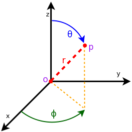
 is the azimuthal orientation of the antenna
(i.e., its direction of maximum gain) and the exponential
is the azimuthal orientation of the antenna
(i.e., its direction of maximum gain) and the exponential
 . Note that
this radiation pattern is independent of the inclination angle
. Note that
this radiation pattern is independent of the inclination angle
 .
.
 is the maximum attenuation in dB of the
antenna. Note that this radiation pattern is independent of the inclination angle
is the maximum attenuation in dB of the
antenna. Note that this radiation pattern is independent of the inclination angle
 determied by the constructor to known reference values. The test
passes if for each case the values are equal to the reference up to a
tolerance of
determied by the constructor to known reference values. The test
passes if for each case the values are equal to the reference up to a
tolerance of  which accounts for numerical errors.
![L_\mathrm{total} = 20\log f + N\log d + L_f(n)- 28 [dB]](_images/math/32fc42c2c4b0e3c21686c34819cb738d54cf215b.png)
 : power loss coefficient [dB]
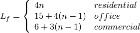
 )
) : frequency [MHz]
 : distance (where
  ) [m]
) [m] , and approximating the number of walls that are penetrated with the manhattan distance (in number of rooms) between the transmitter and the receiver. In detail, let
  ,
,  ,
,  ,
,  denote the room number along the
  and
and  axis respectively for user 1 and 2; the total loss
  is calculated as
 .
. .
.
 ) has to be calculated as the square root of the sum of the quadratic values of the standard deviatio in case of outdoor nodes and the one for the external walls penetration. This is due to the fact that that the components producing the shadowing are independent of each other; therefore, the variance of a distribution resulting from the sum of two independent normal ones is the sum of the variances.
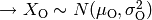
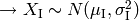
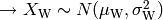
 and variable standard deviation
  , according to models commonly used in literature. Three test cases are provided, which cover the cases of indoor, outdoor and indoor-to-outdoor communications.
Each test case generates 1000 different samples of shadowing for different pairs of MobilityModel instances in a given scenario. Shadowing values are obtained by subtracting from the total loss value returned by
, according to models commonly used in literature. Three test cases are provided, which cover the cases of indoor, outdoor and indoor-to-outdoor communications.
Each test case generates 1000 different samples of shadowing for different pairs of MobilityModel instances in a given scenario. Shadowing values are obtained by subtracting from the total loss value returned by 
 of the fading traces:
![S_{traces} = S_{sample} \times N_{RB} \times \frac{T_{trace}}{T_{sample}} \times N_{scenarios} \mbox{ [bytes]}](_images/math/81abcf57b7823d8e7d7cc6585c5613138ef4ba84.png)
 is the size in bytes of the sample (e.g., 8 in case of double precision, 4 in case of float precision),
  is the number of RB or set of RBs to be considered,
  is the total length of the trace,
  is the time resolution of the trace (1 ms), and
  is the number of fading scenarios that are desired (i.e., combinations of different sets of channel taps and user speed values). We provide traces for 3 different scenarios one for each taps configuration defined in Annex B.2 of
  . All traces have
  s and
s and  . This results in a total 24 MB bytes of traces.
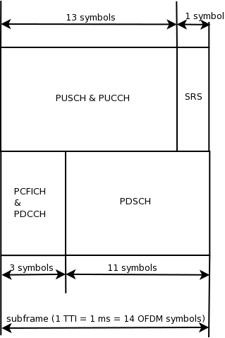
 denote the LTE Absolute Radio Frequency Channel Number, which
identifies the carrier frequency on a 100 kHz raster; furthermore, let
denote the LTE Absolute Radio Frequency Channel Number, which
identifies the carrier frequency on a 100 kHz raster; furthermore, let  used in the simulation we define a corresponding SpectrumModel using
the functionality provided by the
used in the simulation we define a corresponding SpectrumModel using
the functionality provided by the 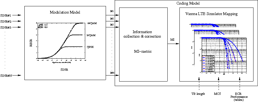
 blocks of size
  and
and  blocks of size
  . Therefore the overall TB BLER (TBLER) can be expressed as
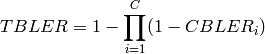
 is the BLER of the CB
 ![CBLER_i = \frac{1}{2}\left[1-erf\left(\frac{x-b_{ECR}}{\sqrt{2}c_{ECR}} \right) \right]](_images/math/f0d47387435f5d86e58f3c7956597437b0276666.png)
 represents the “transition center” and
  is related to the “transition width” of the Gaussian cumulative distribution for each Effective Code Rate (ECR) which is the actual transmission rate according to the channel coding and MCS. For limiting the computational complexity of the model we considered only a subset of the possible ECRs in fact we would have potentially 5076 possible ECRs (i.e., 27 MCSs and 188 CB sizes). On this respect, we will limit the CB sizes to some representative values (i.e., 40, 140, 160, 256, 512, 1024, 2048, 4032, 6144), while for the others the worst one approximating the real one will be used (i.e., the smaller CB size value available respect to the real one). This choice is aligned to the typical performance of turbo codes, where the CB size is not strongly impacting on the BLER. However, it is to be notes that for CB sizes lower than 1000 bits the effect might be relevant (i.e., till 2 dB); therefore, we adopt this unbalanced sampling interval for having more precision where it is necessary. This behaviour is confirmed by the figures presented in the Annes Section.
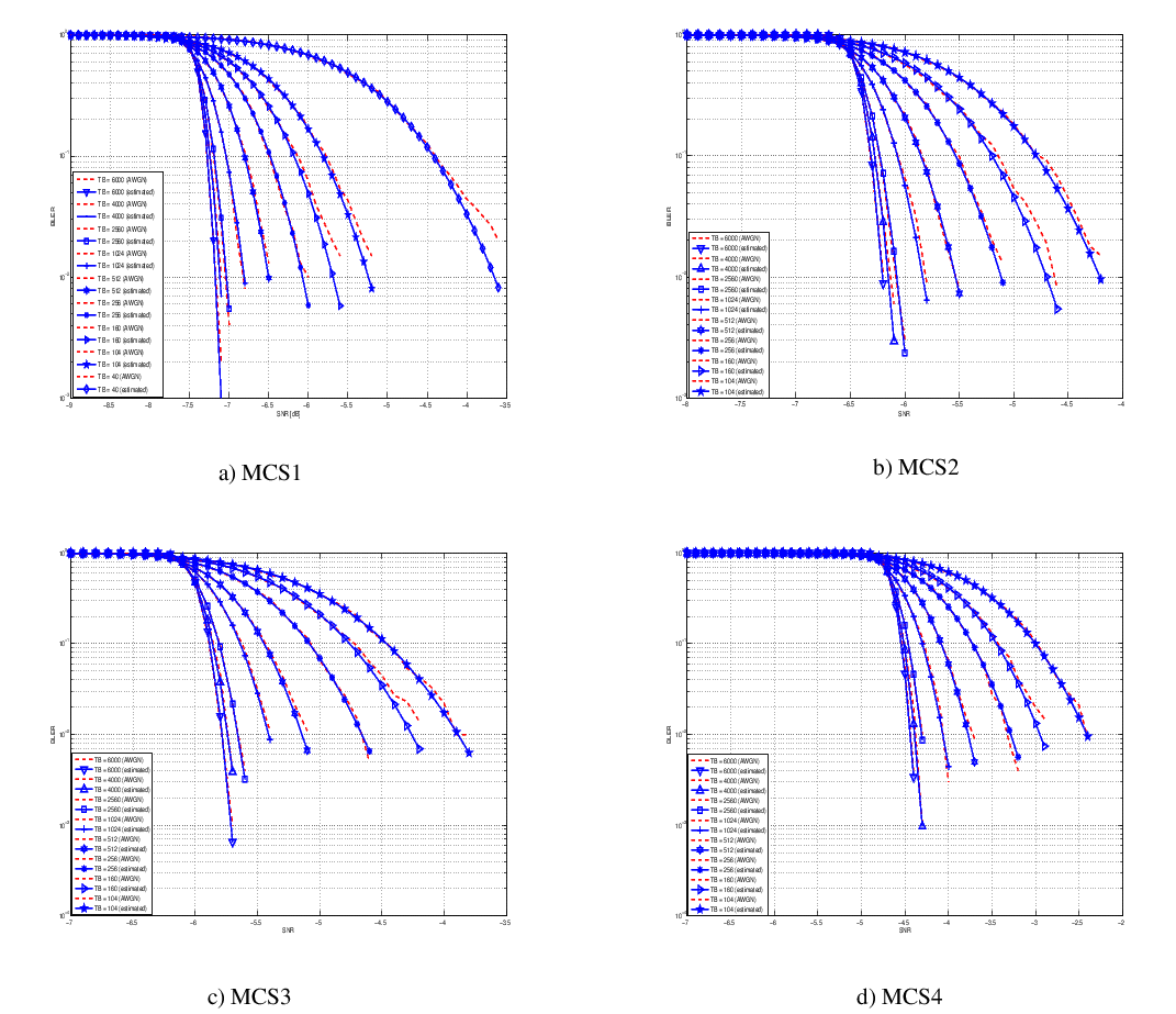
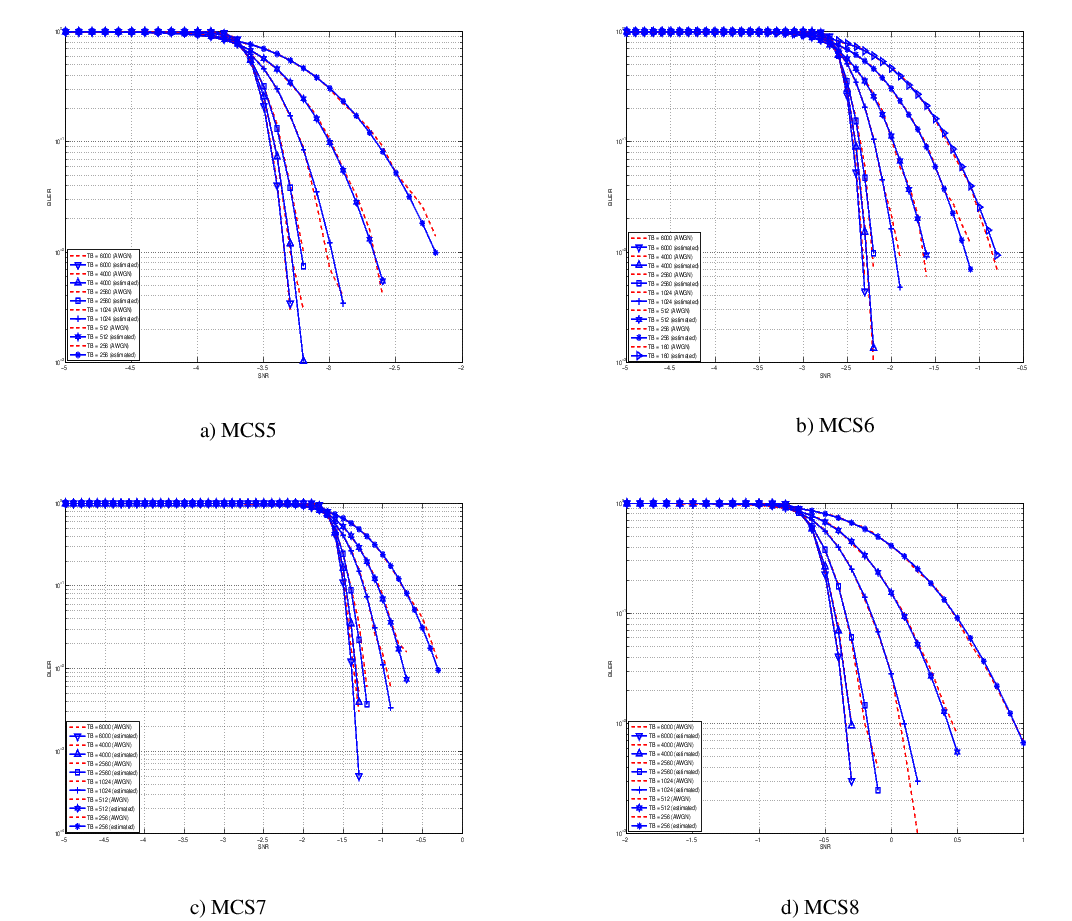
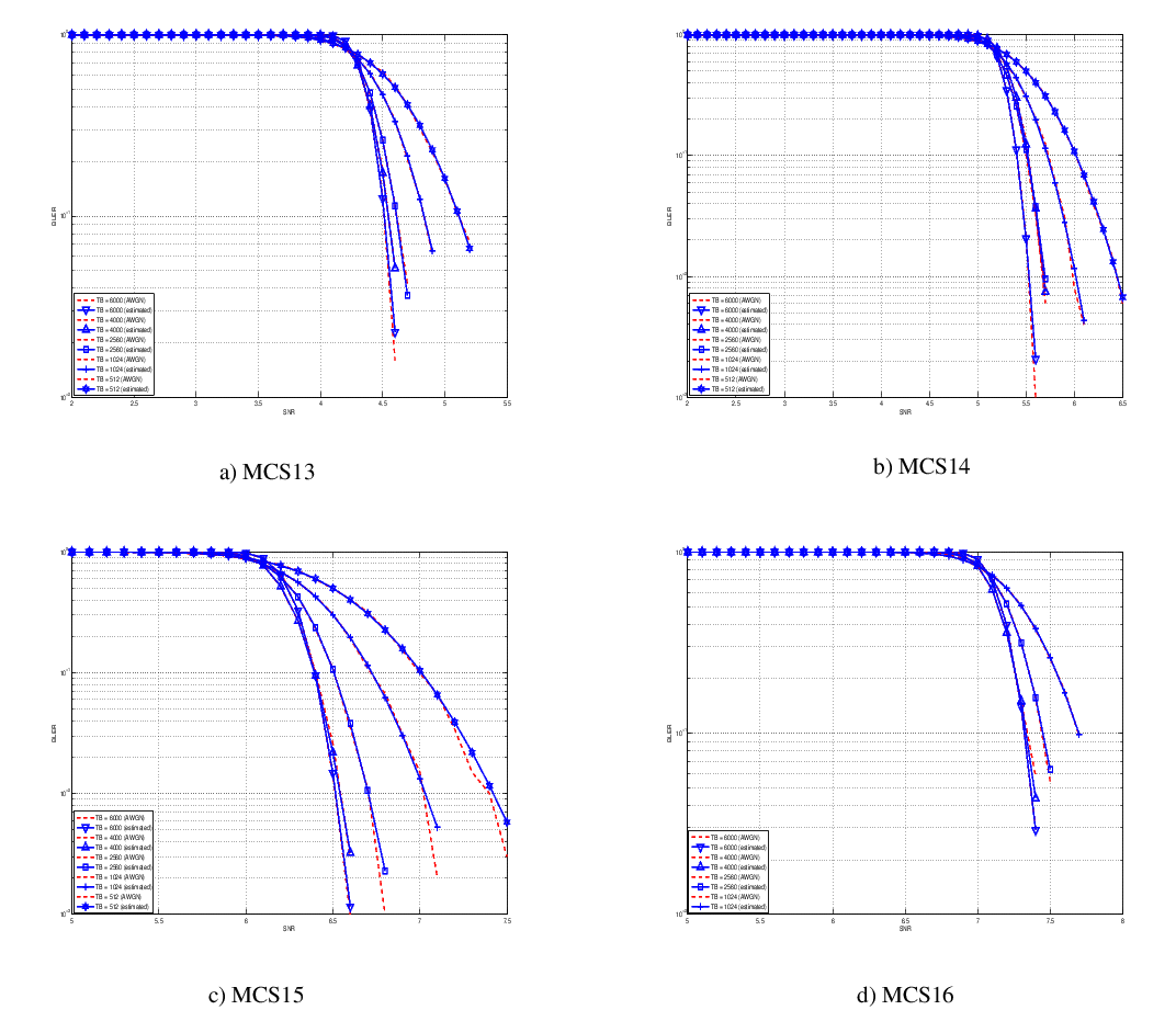
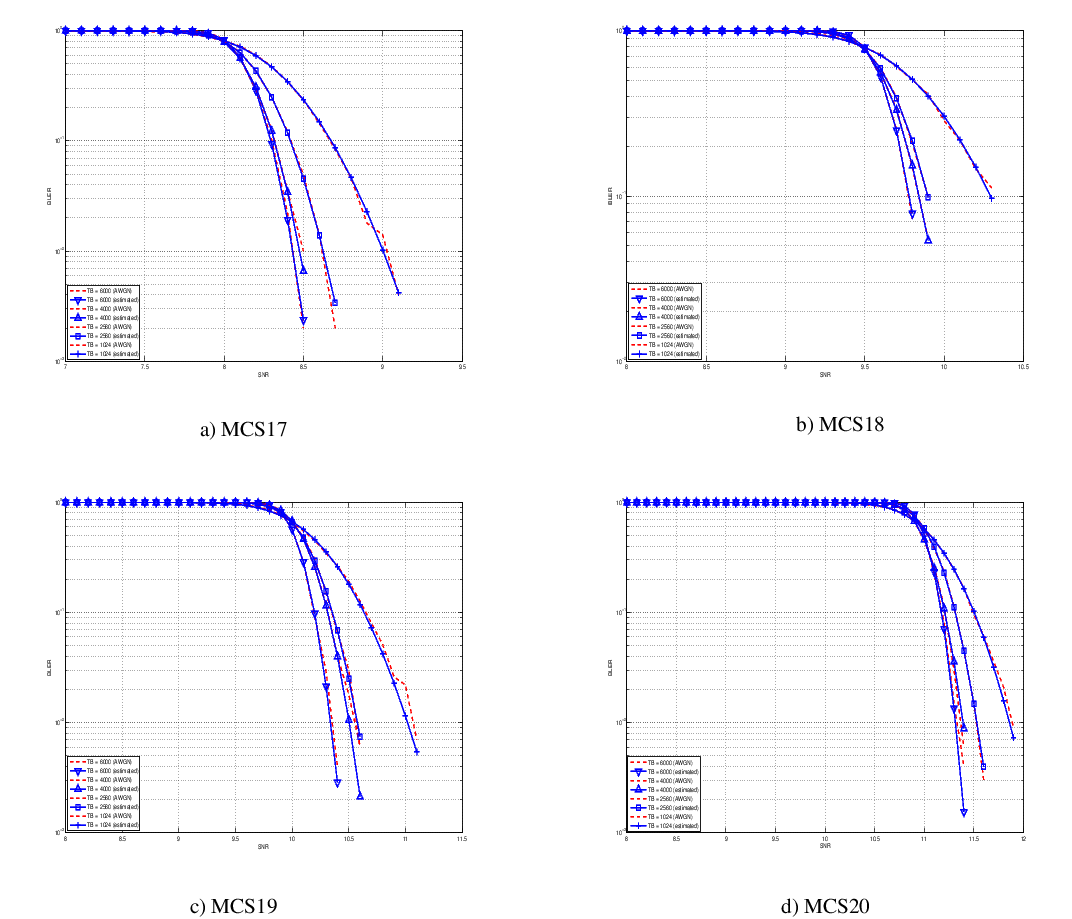
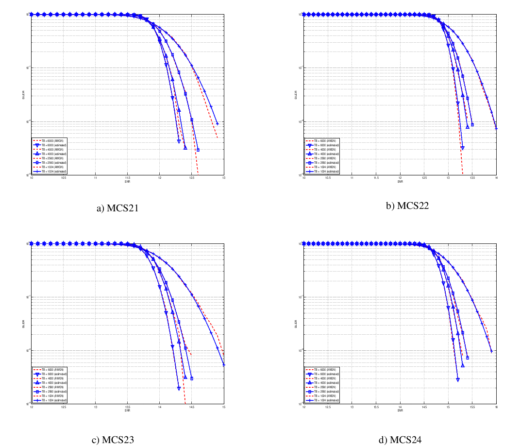
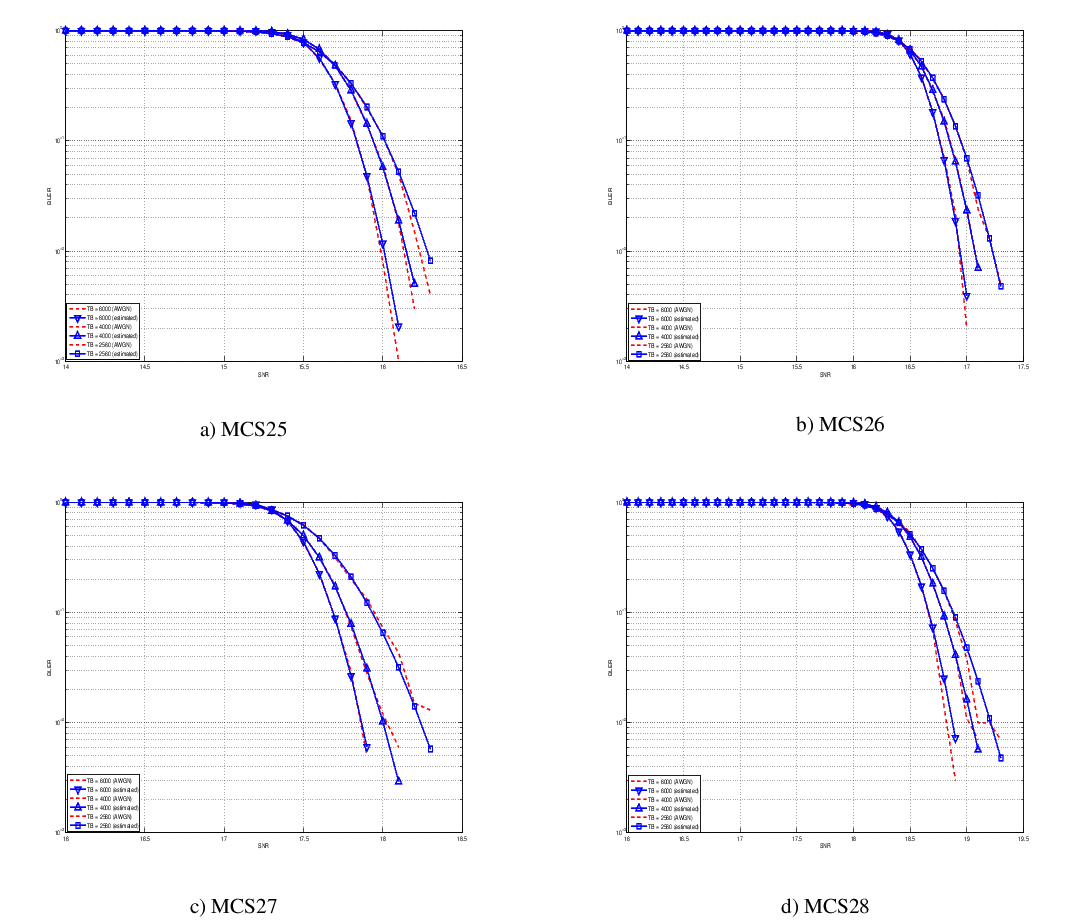
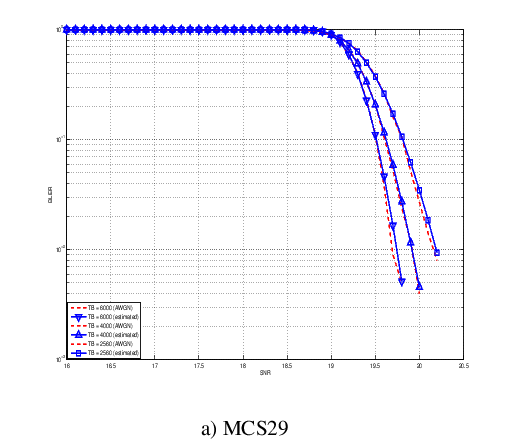
 and
and  [dB].
[dB]. and
and  [dB].
[dB]. and
and  [dB].
[dB]. and
and  [dB].
[dB]. and
and  [dB].
[dB].
 represents the signal power of the RE
  within the RB
  , which, as observed before, is constant within the same RB and equal to
  ,
,  is the number of RBs. It is to be noted that
 is the power spectral density of the RB
  is the bandwidth in Hz of the RB and
  is the number of REs per RB in an OFDM symbol.
Similarly, for RSSI we have
is the number of REs per RB in an OFDM symbol.
Similarly, for RSSI we have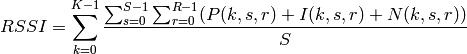
 is the number of OFDM symbols carrying RS in a RB and
  is the number of REs carrying a RS in a OFDM symbol (which is fixed to
  ) while
  ,
,  and
and  represent respectively the perceived power of the serving cell, the interference power and the noise power of the RE
  . As for RSRP, the measurements within a RB are always equals among each others according to the PHY model; therefore
  ,
,  and
and 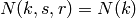 , which implies that the RSSI can be calculated as:
 as detailed in the following:
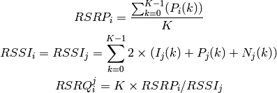
 is the RSRP of the neighbor cell
  is the power perceived at any RE within the RB
  is the RSSI of the neighbor cell
  ),
),  is the total interference perceived by UE in any RE of RB
  is the power perceived of cell
 ![\in [0..9]](_images/math/4fafec854b76790da0793c55a3947ff2ffd7f73a.png) , 16QAM for MCS
, 16QAM for MCS ![\in [10..16]](_images/math/d5d9cf0fbd9960caf5e9ceeae1ad3e98b80e9929.png) and 64QAM for MCS
and 64QAM for MCS ![\in [17..28]](_images/math/146086d4046154939d3d1b86351f6b878c775aec.png) ). This restriction comes from the specification of the rate matcher in the 3GPP standard
). This restriction comes from the specification of the rate matcher in the 3GPP standard 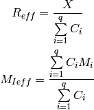
 is the number of original information bits,
  are number of coded bits,
  retransmissions. Therefore, in order to be able to return the error probability with the error model implemented in the simulator evaluates the
  and the
  and return the value of error probability of the ECR of the same modulation with closest lower rate respect to the
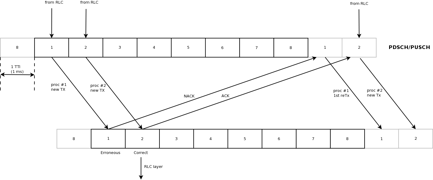
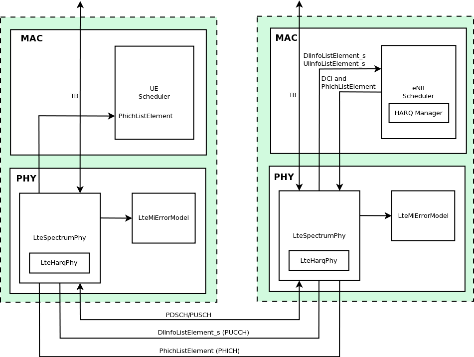
 be its SINR. We get the spectral efficiency
 of user
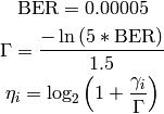
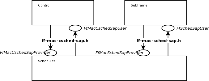
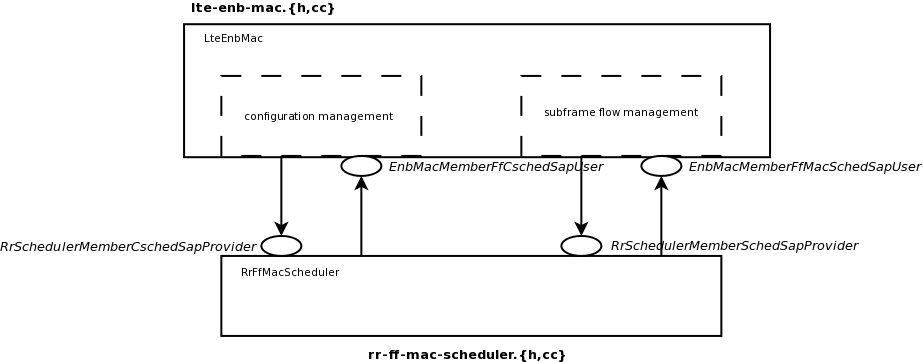
 denote generic users; let
  be the
subframe index, and
be the
subframe index, and  be MCS
usable by user
be MCS
usable by user  in bit/s for user
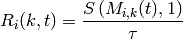
 to which RBG
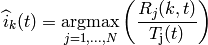
 is the past througput performance perceived by the
user
is the past througput performance perceived by the
user 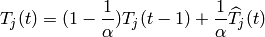
 is the time constant (in number of subframes) of
the exponential moving average, and
is the time constant (in number of subframes) of
the exponential moving average, and  is the actual
throughput achieved by the user
is the actual
throughput achieved by the user  actually used by user
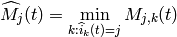
 of RBGs allocated to user
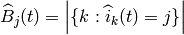
 indicates the cardinality of the set; finally,
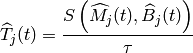
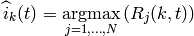
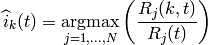
 in bit/s stands
for the achievable rate for
in bit/s stands
for the achievable rate for 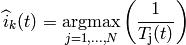
 : packet arrival rate (byte/sec )
 : token generation rate (byte/sec)
 : token pool size (byte)
 : counter that records the number of token borrowed from or given to the token bank by flow
  , and
, and  : if
: if  : the maximum number of tokens UE i can borrow from the bank in one time.
 : once
  UEs with
highest metric in two sets and forward those UE to FD scheduler. In PSS, FD scheduler allocates RBG k to UE n
that maximums the chosen metric. Two PF schedulers are used in PF scheduler:
UEs with
highest metric in two sets and forward those UE to FD scheduler. In PSS, FD scheduler allocates RBG k to UE n
that maximums the chosen metric. Two PF schedulers are used in PF scheduler: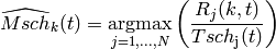
![\widehat{Mcoi}_{k}(t) = \underset{j=1,...,N}{\operatorname{argmax}}
\left( \frac{ CoI[j,k] }{ \sum_{k=0}^{N_{RBG}} CoI[j,k] } \right)](_images/math/bccad3d0b042ccded9075ad344f556d1f5c5af3f.png)
 is similar past throughput performance perceived by the user
 ![CoI[j,k]](_images/math/d8d9a5dcf33c2c696c836e050fba54c751ceee0e.png) is an
estimation of the SINR on the RBG
is an
estimation of the SINR on the RBG ![W[n] = max (1, \frac{TBR}{ T_{j}(t) })](_images/math/178da7df700ae55ea5ca8f9ec708f75de9377ee4.png)
 ,
,  ) by weight
 ![W[n]](_images/math/eab11fe17c20800f593fccf794140aba35ea4f58.png) . This strategy will guarantee the throughput of lower
quality UE tend towards the TBR.
. This strategy will guarantee the throughput of lower
quality UE tend towards the TBR. for user
  is defined in the
following way:
is defined in the
following way: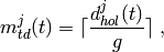
 is the current value of HOL delay of flow
 is a grouping parameter that determines
granularity of the groups, i.e. the number of the flows that will be
considered in the FD scheduling iteration.
is a grouping parameter that determines
granularity of the groups, i.e. the number of the flows that will be
considered in the FD scheduling iteration. , the CQA scheduler
assigns the current RBG to the user
, the CQA scheduler
assigns the current RBG to the user 
 is calculated as follows:
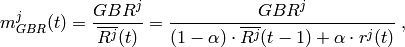
 is the bit rate specified in EPS bearer of the
flow
is the bit rate specified in EPS bearer of the
flow  is the past averaged throughput that is calculated with a
moving average,
is the past averaged throughput that is calculated with a
moving average,  is the throughput achieved at the
time t, and
is the throughput achieved at the
time t, and  .
. we consider two different
metrics:
we consider two different
metrics:  and
and  .
.
 is the Proportional Fair metric which is defined as follows:
 is the estimated achievable throughput of user
 which
is proposed in
which
is proposed in 
 is the last reported CQI value from user
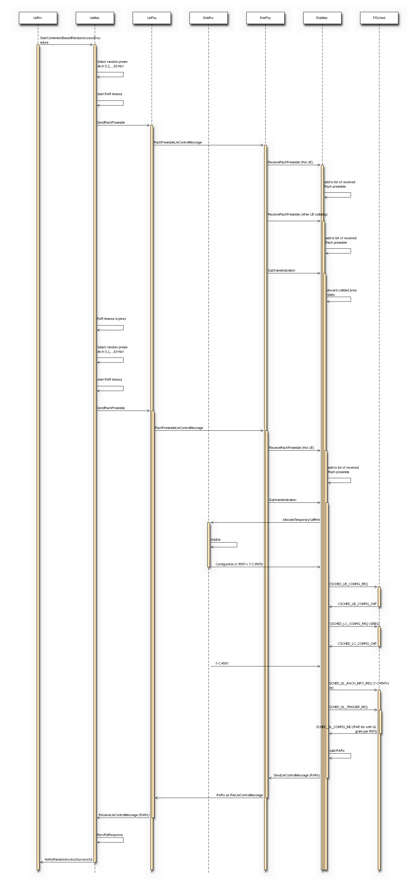
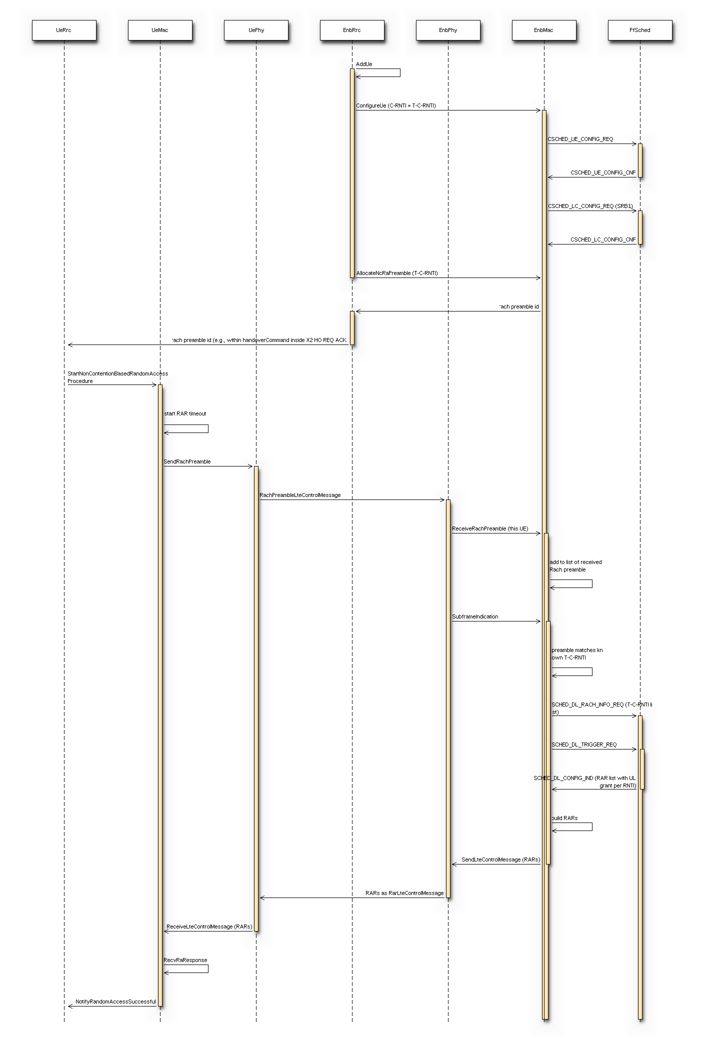
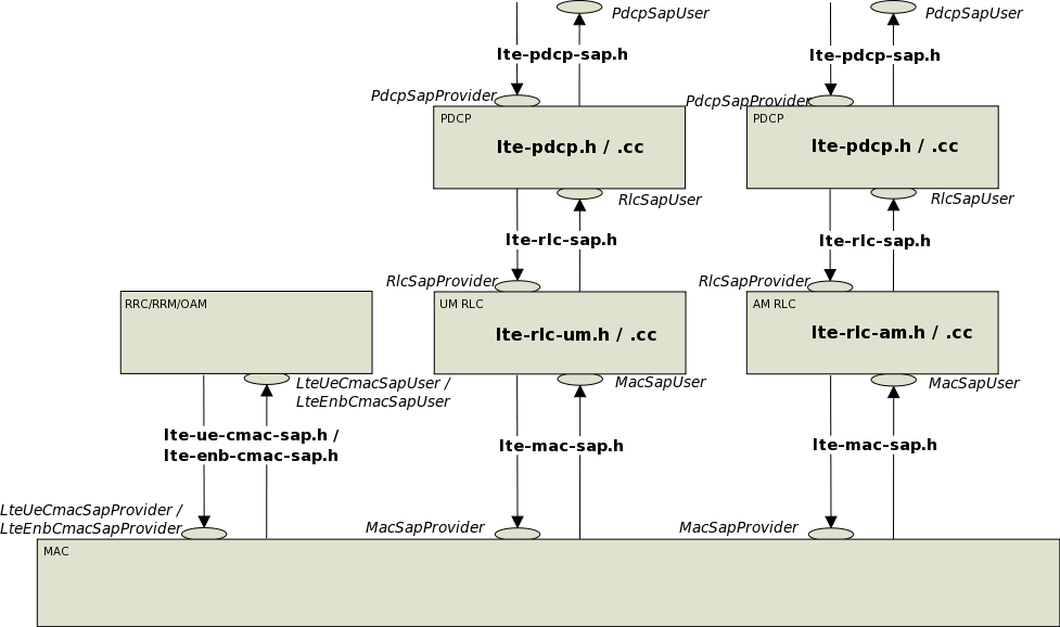
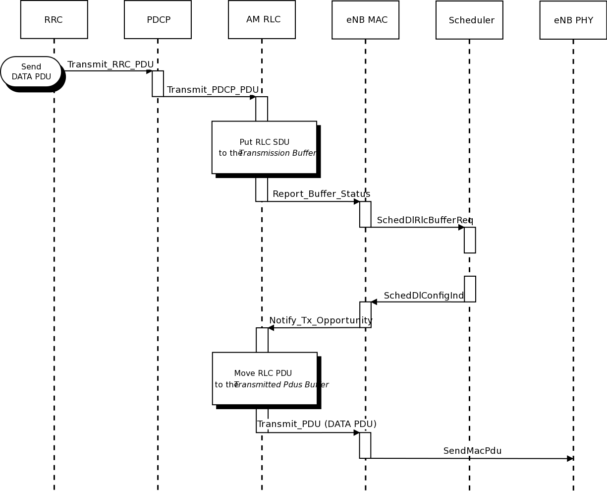
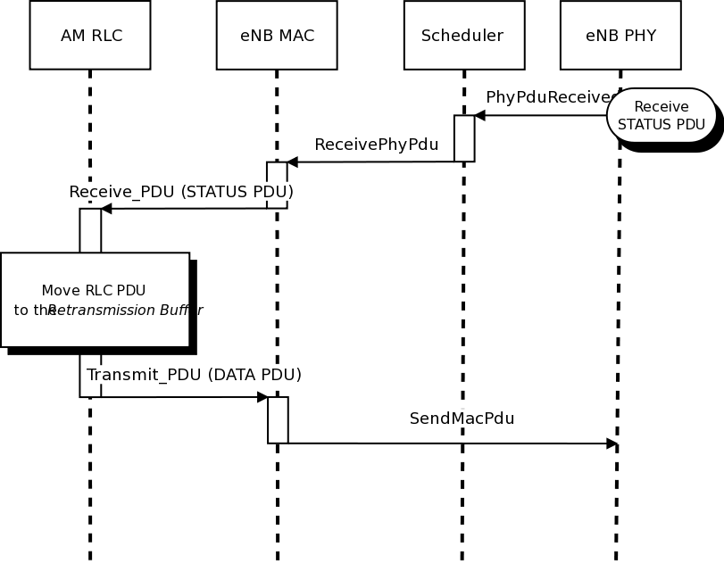
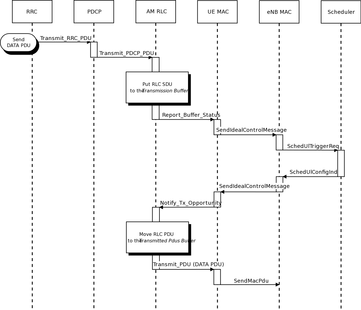
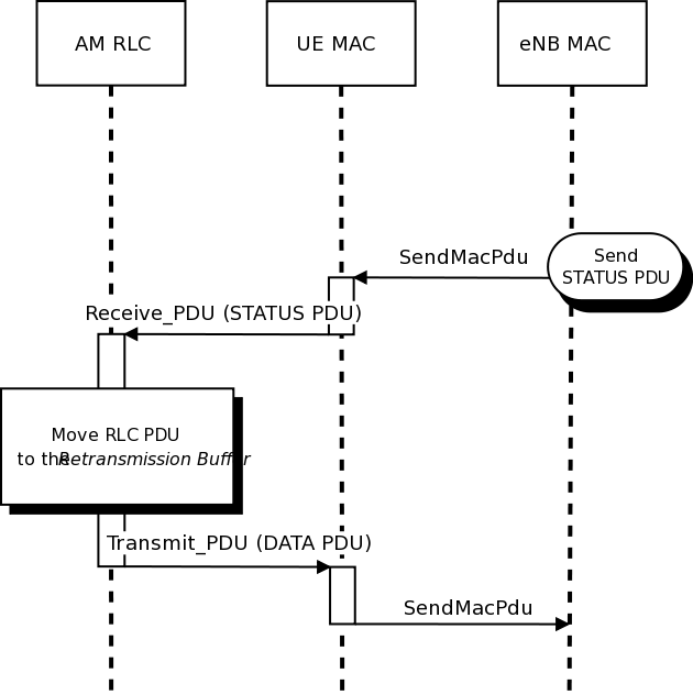
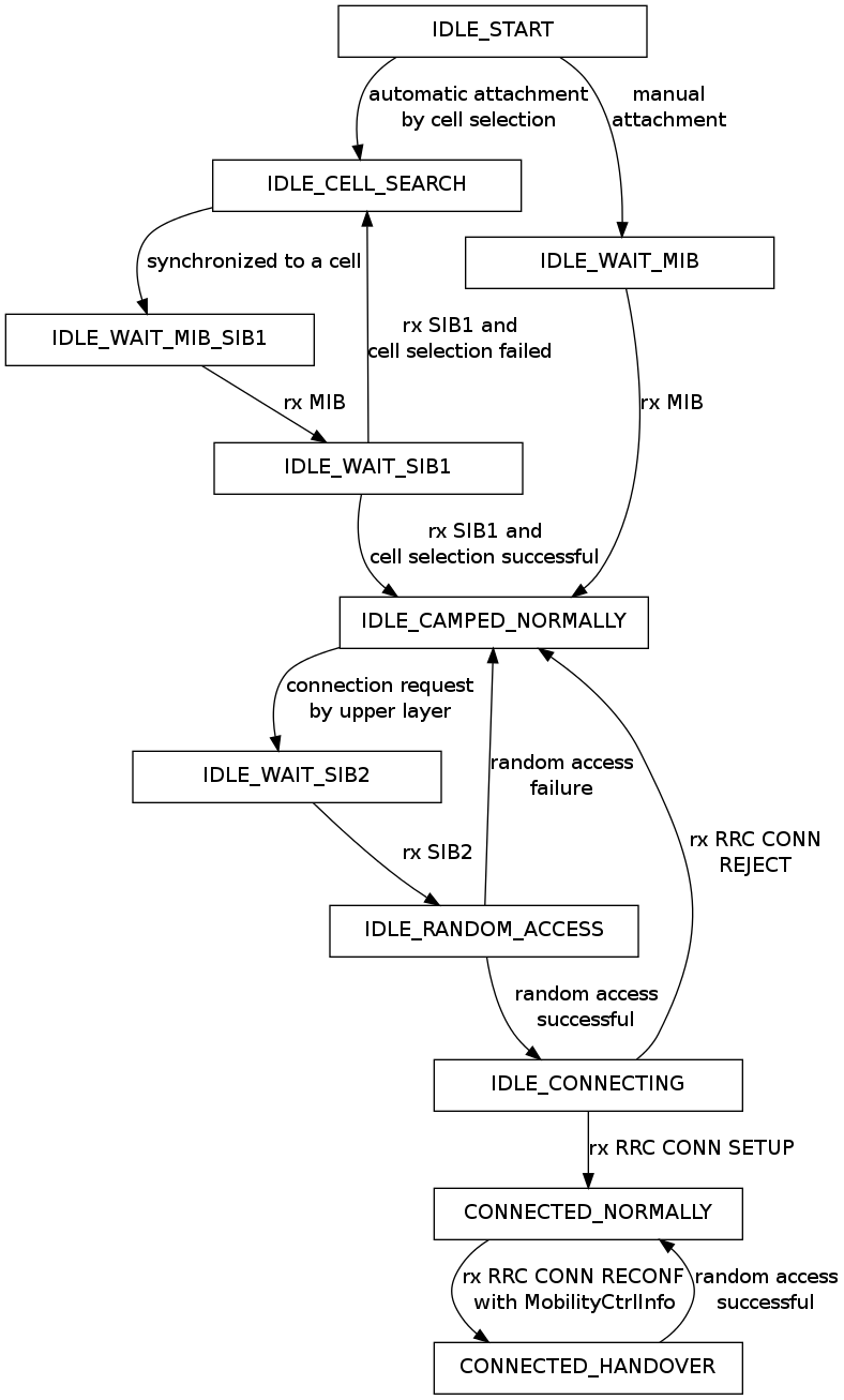
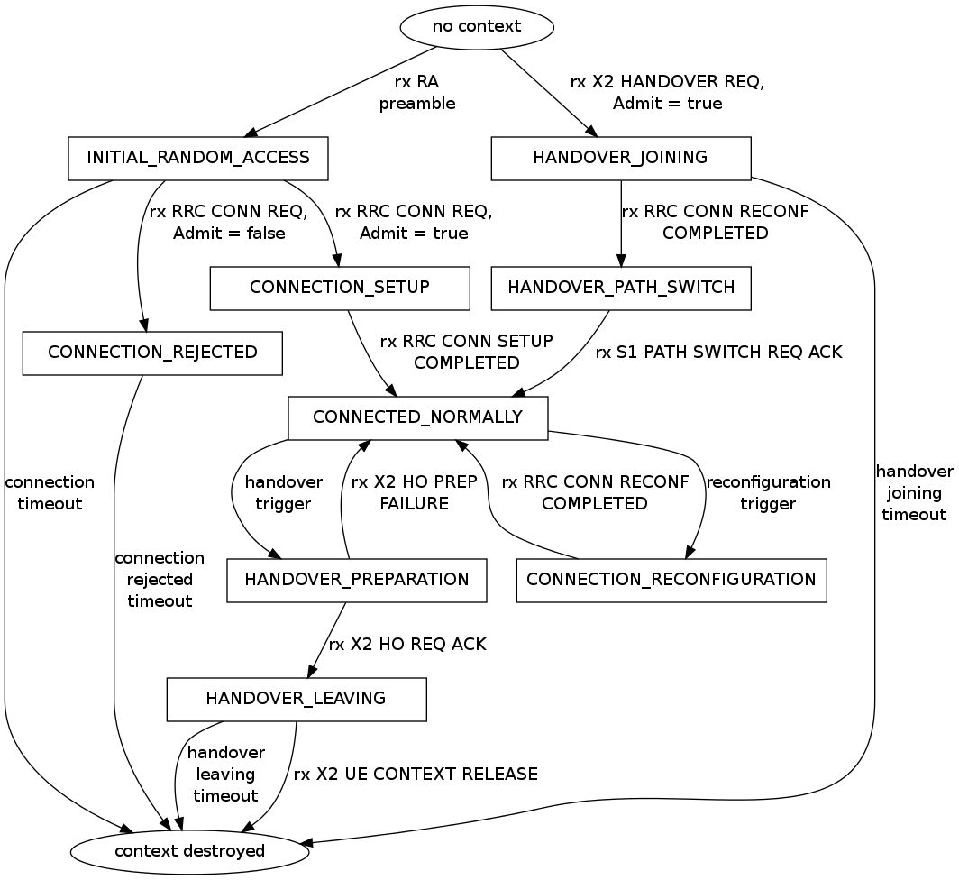
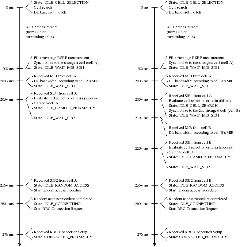
 , which has to be higher than a required minimum
 in order to pass the criterion:
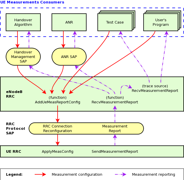

 is the latest received measurement result from the physical
layer;
is the latest received measurement result from the physical
layer; is the updated filtered measurement result;
 is the old filtered measurement result, where
 (i.e. the first measurement is not filtered); and
 , where
  is the default value, but can be configured by setting the
RsrpFilterCoefficient and RsrqFilterCoefficient attributes in
is the default value, but can be configured by setting the
RsrpFilterCoefficient and RsrqFilterCoefficient attributes in
 will disable Layer 3 filtering. On the other hand, past
measurements can be granted more influence on the filtering results by using
larger value of
will disable Layer 3 filtering. On the other hand, past
measurements can be granted more influence on the filtering results by using
larger value of  ) defines the distance between the
entering and leaving conditions in dB. Similarly, time-to-trigger introduces
delay to both entering and leaving conditions, but as a unit of time.
) defines the distance between the
entering and leaving conditions in dB. Similarly, time-to-trigger introduces
delay to both entering and leaving conditions, but as a unit of time. and
and  in Event A3, A4, and A5) are not
supported as well. The value equal to zero is always assumed in place of them.
in Event A3, A4, and A5) are not
supported as well. The value equal to zero is always assumed in place of them.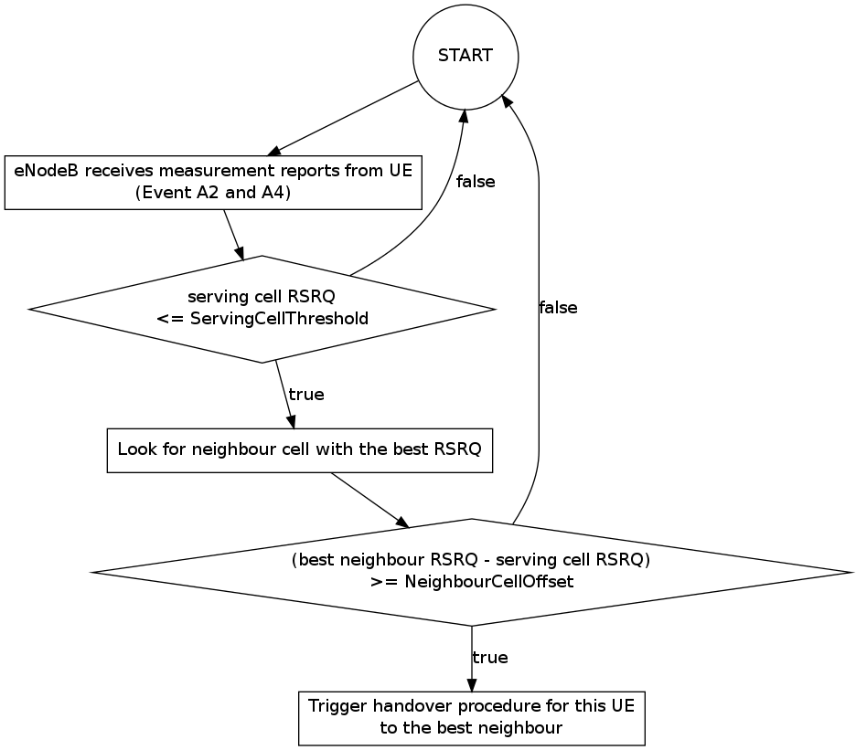
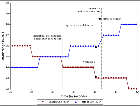
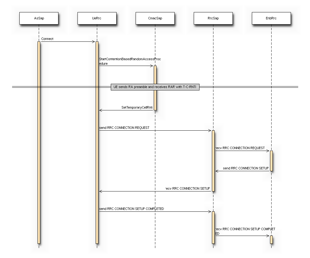
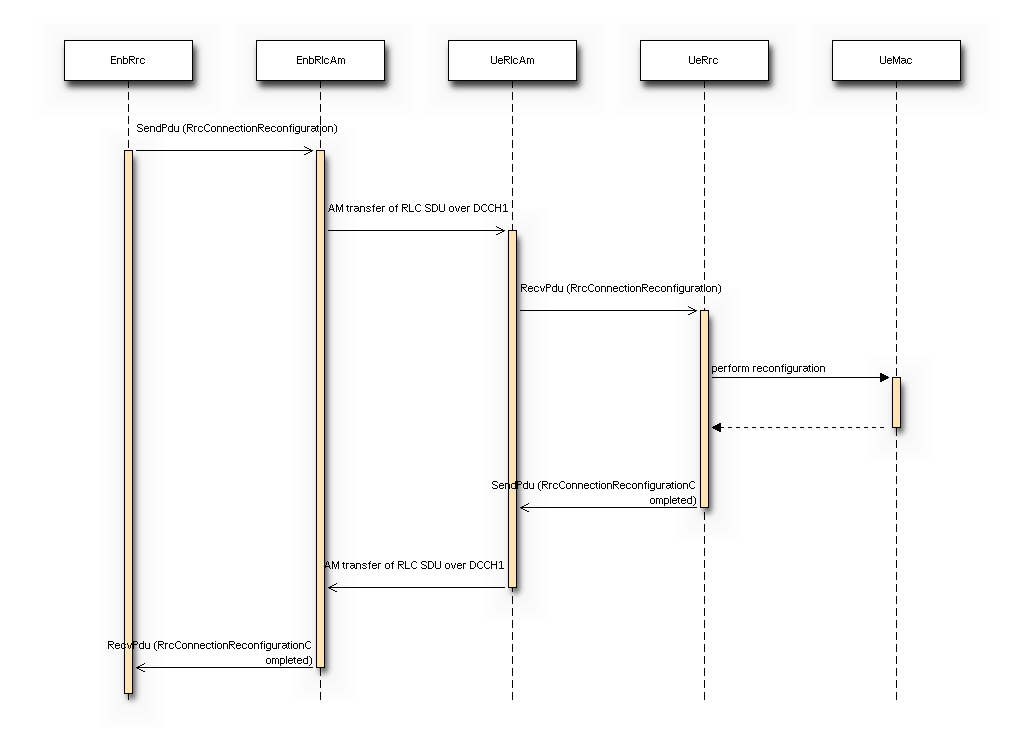
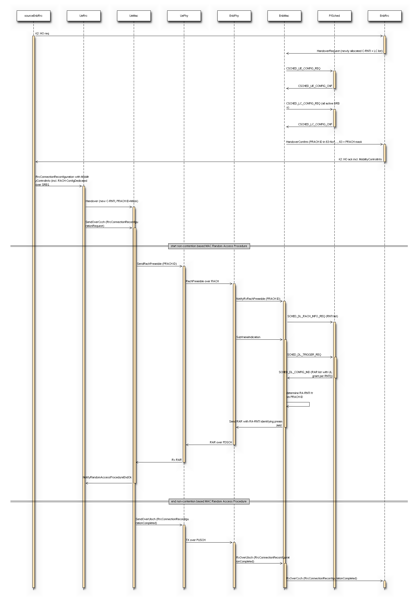
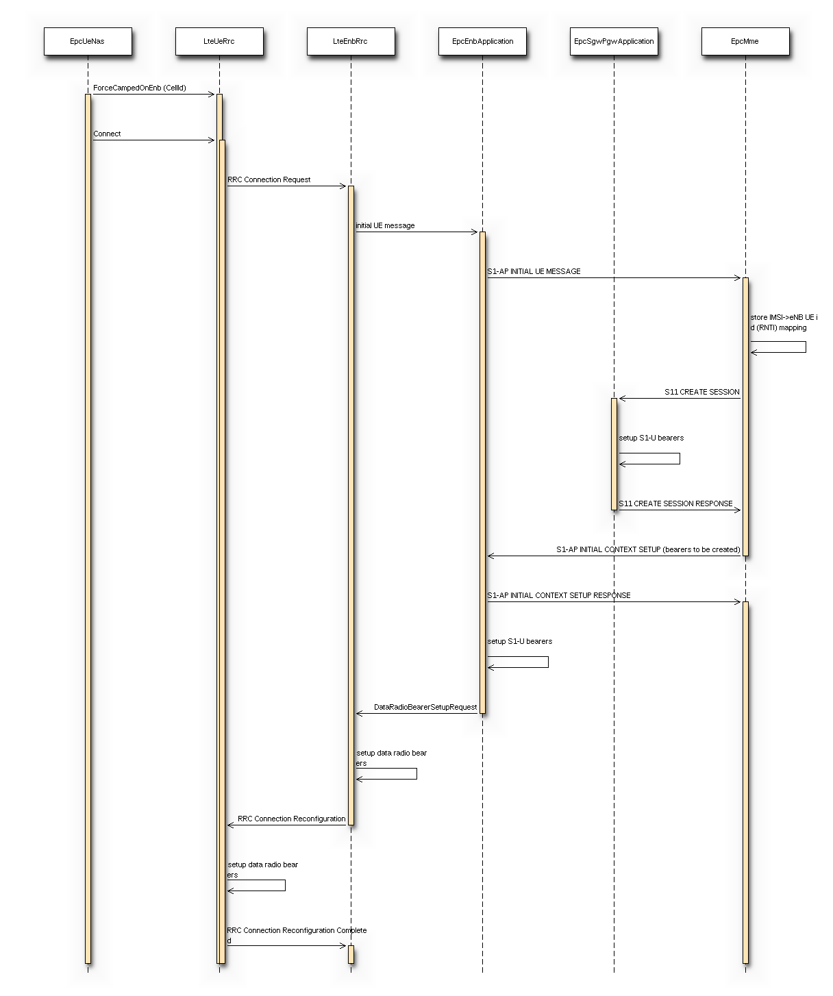
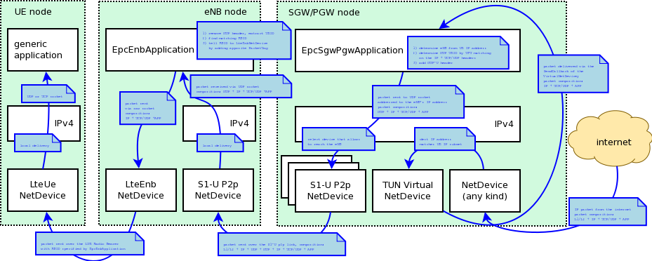
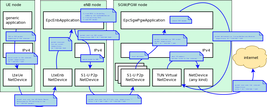
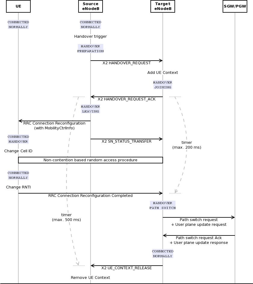
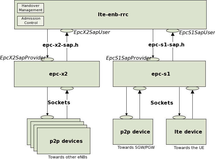
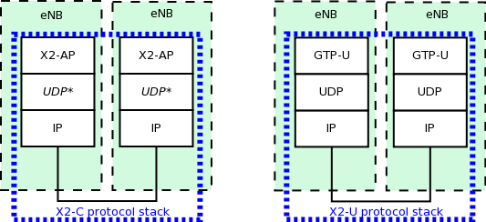
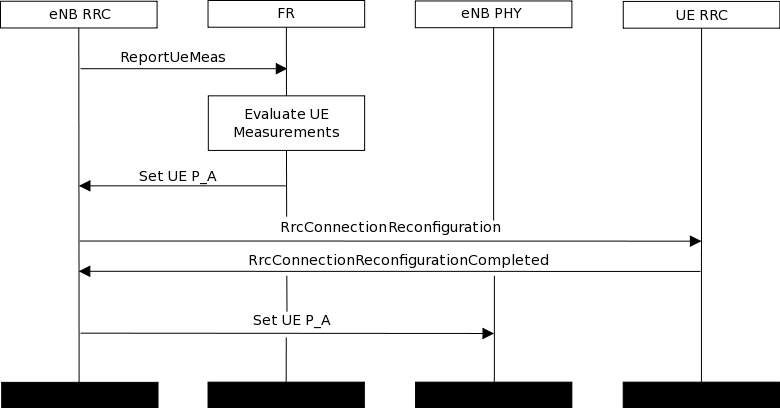
 for PUSCH transmission in subframe
 ![P_{PUSCH,c}(i)=\min\begin{Bmatrix}
P_{CMAX,c}(i)\\
10\log_{10}(M_{PUSCH,c}(i))+ P_{O\_PUSCH,c}(j)
+ \alpha_{c} (j) * PL_{c} + \Delta_{TF,c}(i) + f_{c}(i)
\end{Bmatrix} [dBm]](_images/math/a7a7ba250fad2e583af980de15edd12d6736364c.png)
![P_{PUSCH,c}(i)=\min\begin{Bmatrix}
10\log_{10}(\hat{P}_{CMAX,c}(i) - \hat{P}_{PUCCH}(i))\\
10\log_{10}(M_{PUSCH,c}(i))+ P_{O\_PUSCH,c}(j)
+ \alpha_{c} (j) * PL_{c} + \Delta_{TF,c}(i) + f_{c}(i)
\end{Bmatrix} [dBm]](_images/math/1cd5612313ef0cbc814d41ab1ffe83704abefb9b.png)
![P_{PUSCH,c}(i)=\min\begin{Bmatrix}
{P}_{CMAX,c}(i)\\
P_{O\_PUSCH,c}(1) + \alpha_{c} (1) * PL_{c} + f_{c}(i)
\end{Bmatrix} [dBm]](_images/math/d73151c47b993e6d3c57b9ee683539a590304cda.png)
 is the configured UE transmit power defined in 3GPP 36.101. Table 6.2.2-1
in subframe
is the configured UE transmit power defined in 3GPP 36.101. Table 6.2.2-1
in subframe  is the linear
value of
is the linear
value of  is the bandwidth of the PUSCH resource assignment expressed in number
of resource blocks valid for subframe
is the bandwidth of the PUSCH resource assignment expressed in number
of resource blocks valid for subframe  is a parameter composed of the sum of a component
  provided from higher layers for
  and a component
  provided by higher
layers for
provided by higher
layers for  is a 3-bit parameter provided by higher layers for serving cell
  ,
,  For
For  ,
,  .
This parameter is configurable by attribute system:
.
This parameter is configurable by attribute system: is the downlink pathloss estimate calculated in the UE for serving cell
  , where
  is provided by higher layers and RSRP.
  for
for  and
and  for
for  . Only second case is implemented.
 is component of Closed Loop Power Control. It is the current PUSCH power control
adjustment state for serving cell
is component of Closed Loop Power Control. It is the current PUSCH power control
adjustment state for serving cell 
 is a correction value, also referred to as a TPC command and is included
in PDCCH with DCI;
is a correction value, also referred to as a TPC command and is included
in PDCCH with DCI;  was signalled on PDCCH/EPDCCH with DCI for
serving cell
was signalled on PDCCH/EPDCCH with DCI for
serving cell  ;
;  for FDD.
 for the SRS transmitted on subframe
 ![P_{PUSCH,c}(i)=\min\begin{Bmatrix}
{P}_{CMAX,c}(i)\\
P_{SRS\_OFFSET,c}(m) + 10\log_{10}(M_{SRS,c})+
P_{O\_PUSCH,c}(j) + \alpha_{c}(j) * PL_{c} + f_{c}(i)
\end{Bmatrix} [dBm]](_images/math/efd0dc8debafe094a612dedbc5b59952cecb0301.png)
 is semi-statically configured by higher layers for
  for
serving cell
for
serving cell  .
For
.
For ![P_{SRS\_OFFSET,c}(m)value = -10.5 + P_{SRS\_OFFSET,c}(m) * 1.5 [dBm]](_images/math/f6193214612e33a37d38fa85827e3cc2637fd37d.png)
 is the bandwidth of the SRS transmission in subframe
  are parameters as defined in
 .
.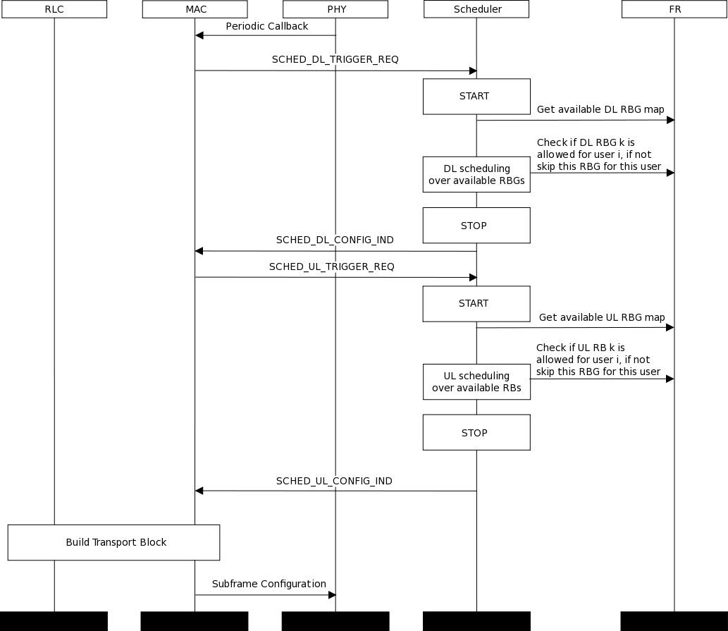
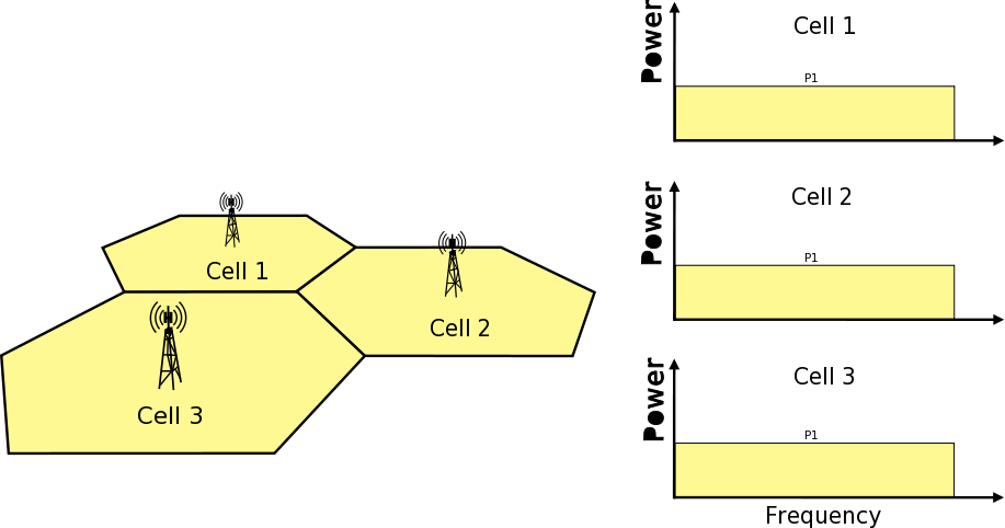
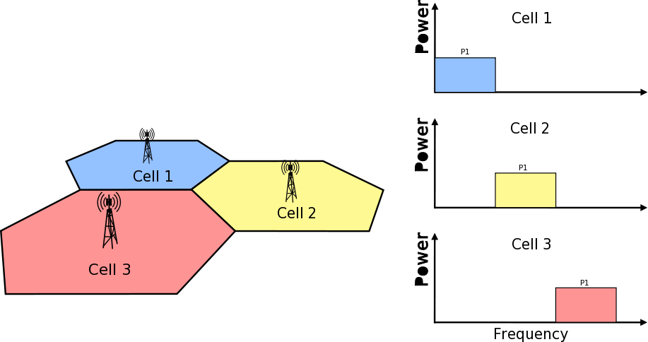
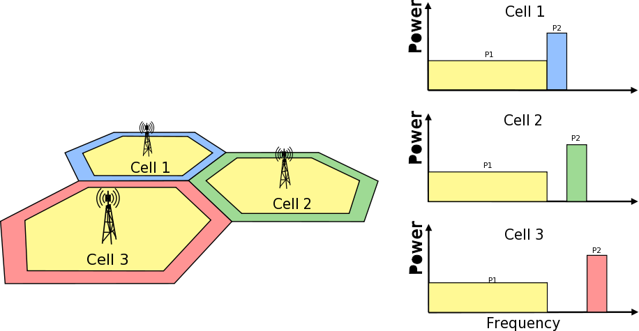
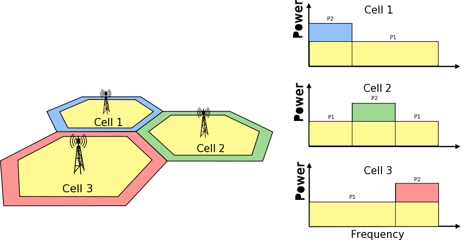
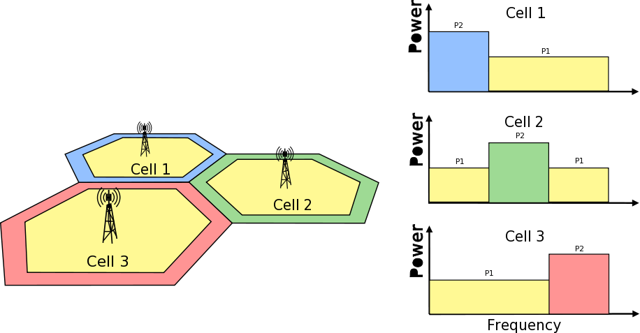
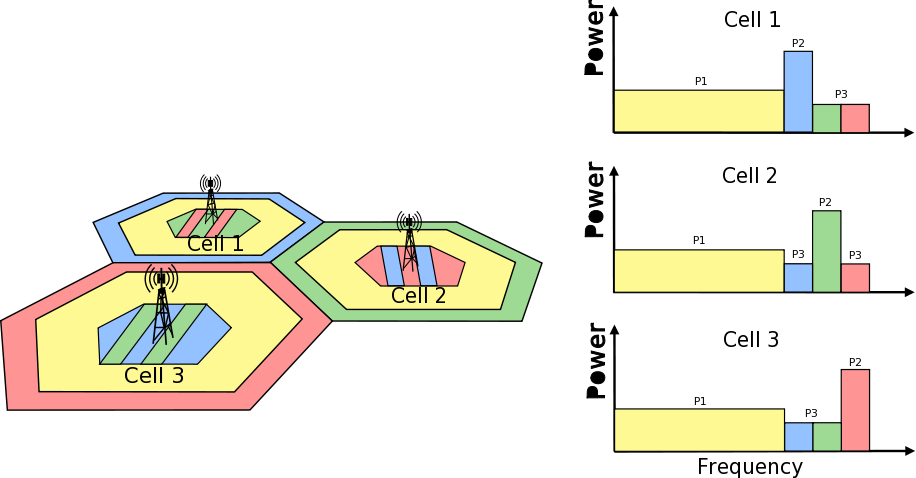
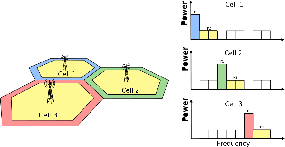
 for each RB.
 is a set of neighbor cells,
  is the RNTP from the
  denotes weight with respect to adjacent
cell
denotes weight with respect to adjacent
cell 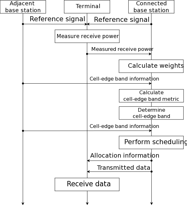
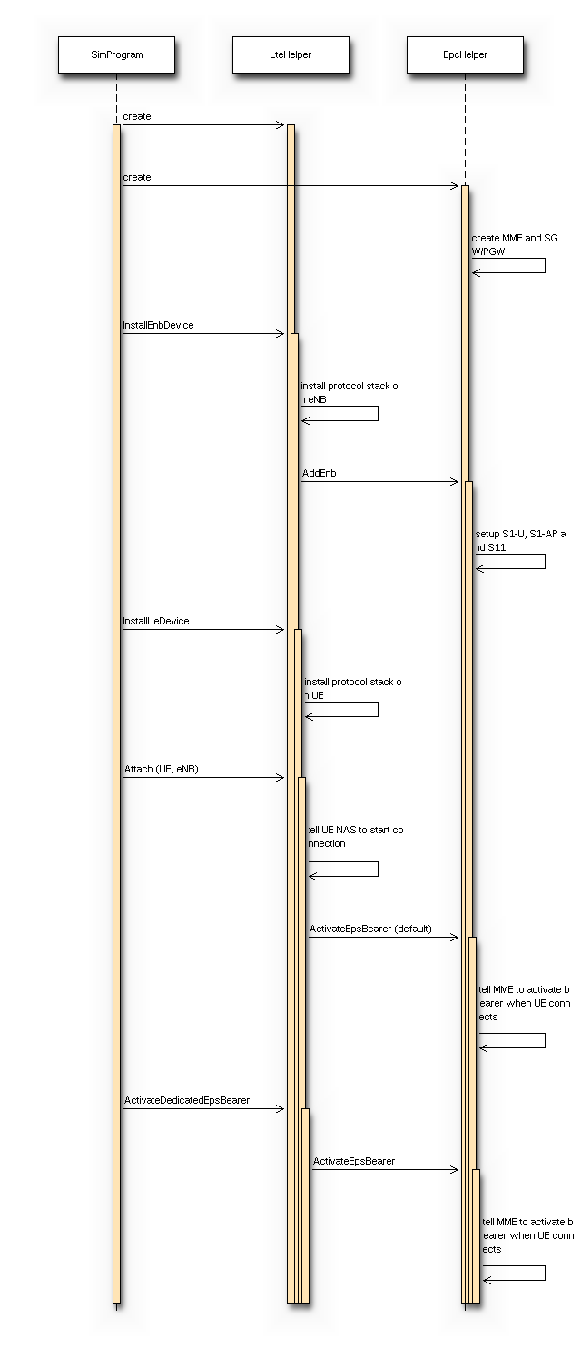
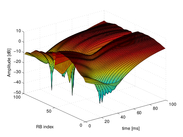
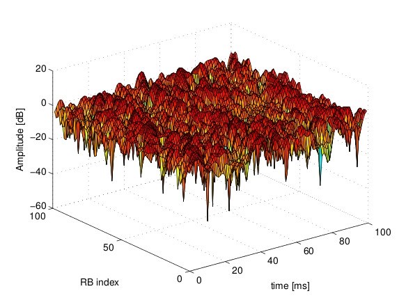
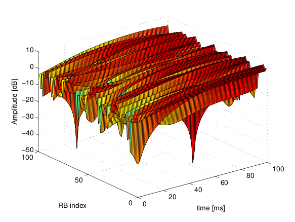
 degrees from the direction of orientation is -3 dB.
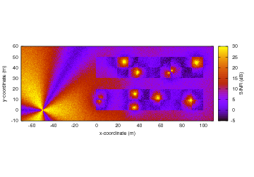
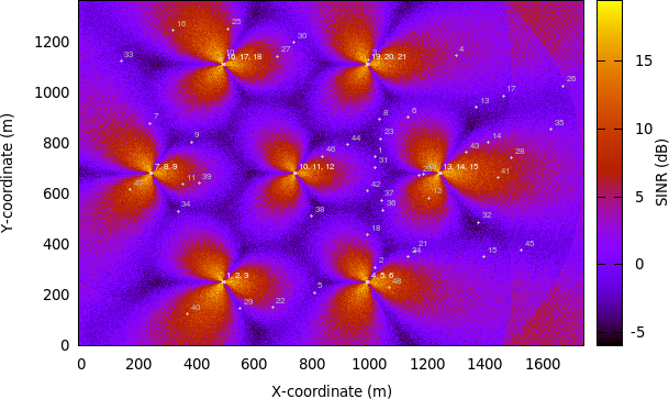
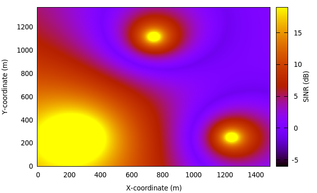
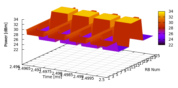
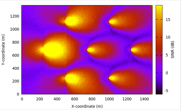
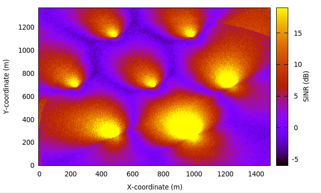
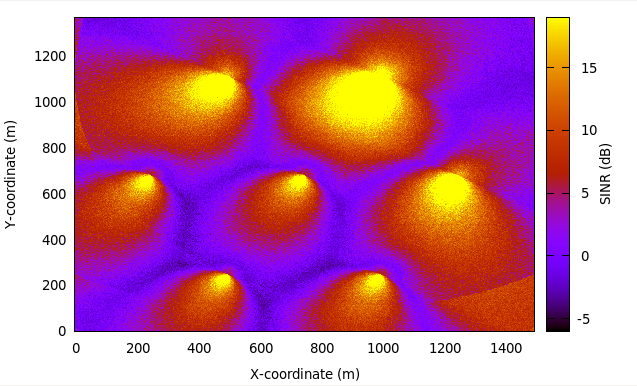
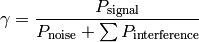
 its SINR,
calculated with the above equation. The calculation of the average
SINR
its SINR,
calculated with the above equation. The calculation of the average
SINR  to be used for CQI feedback reporting
uses the following formula:
to be used for CQI feedback reporting
uses the following formula:
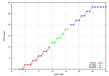
 parameter represents the distance of each UE to the eNB it
is attached to, whereas the
parameter represents the distance of each UE to the eNB it
is attached to, whereas the  parameter represent the
interferer distance. We note that the scenario topology is such that
the interferer distance is the same for uplink and downlink; still,
the actual interference power perceived will be different, because of
the different propagation loss in the uplink and downlink
bands. Different test cases are obtained by varying the
parameter represent the
interferer distance. We note that the scenario topology is such that
the interferer distance is the same for uplink and downlink; still,
the actual interference power perceived will be different, because of
the different propagation loss in the uplink and downlink
bands. Different test cases are obtained by varying the 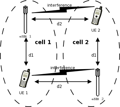
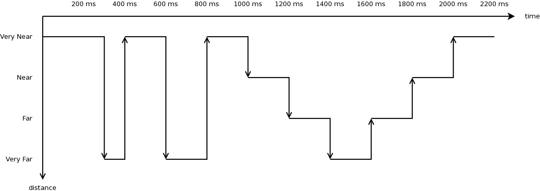
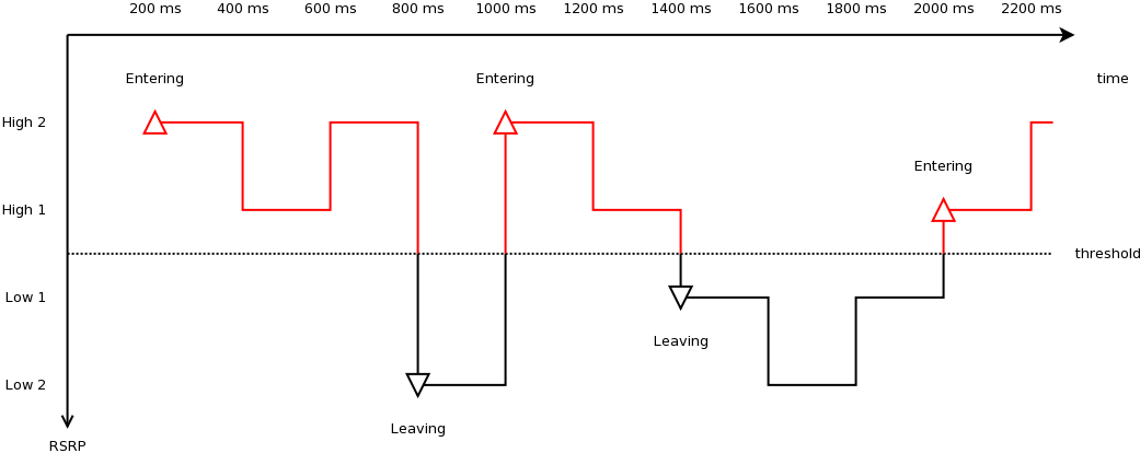
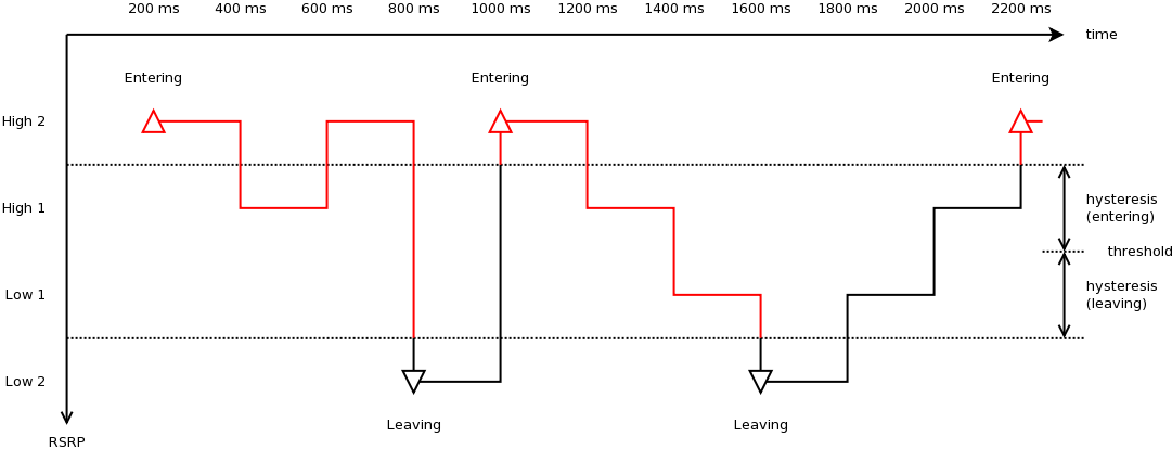
 the RBG size,
  of RBGs allocated to each user as
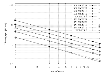
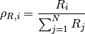
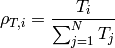


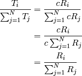
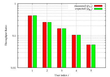

 in PFsch or same
 ![CoI[k,n]](_images/math/a5b3239801c9ee2c99c3cca44ad11e11700a0c48.png) in CoItA. This means that PSS will performs like a
TD-BET which allocates all RBGs to one UE in each TTI. Then the maximum value of UE throughput equals to
the achievable rate that all RBGs are allocated to this UE.
in CoItA. This means that PSS will performs like a
TD-BET which allocates all RBGs to one UE in each TTI. Then the maximum value of UE throughput equals to
the achievable rate that all RBGs are allocated to this UE.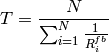
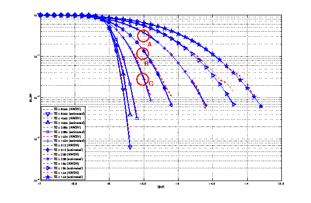
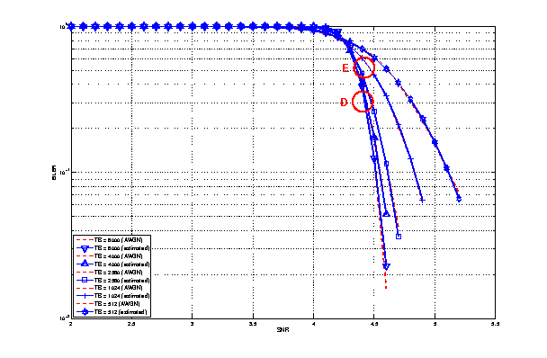

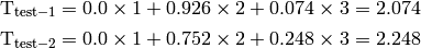
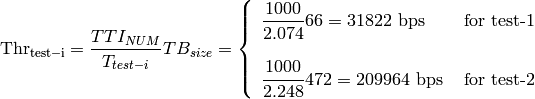

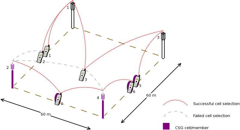
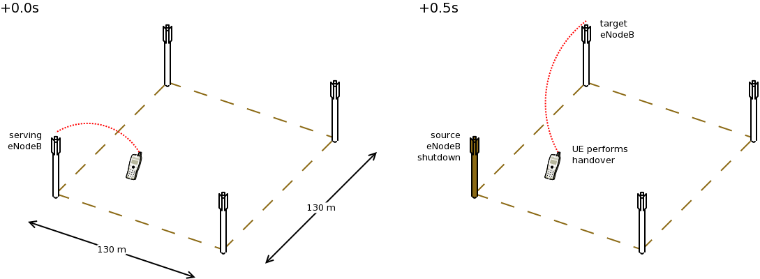
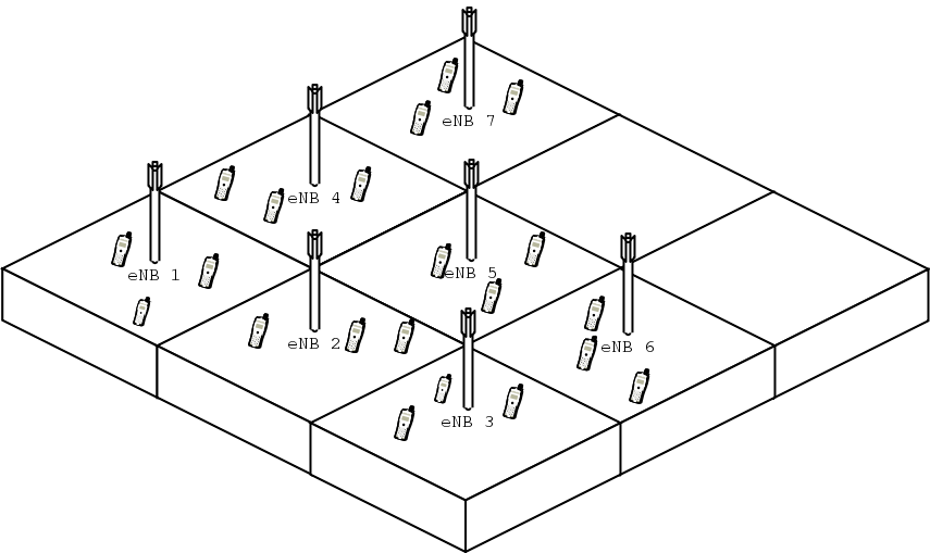
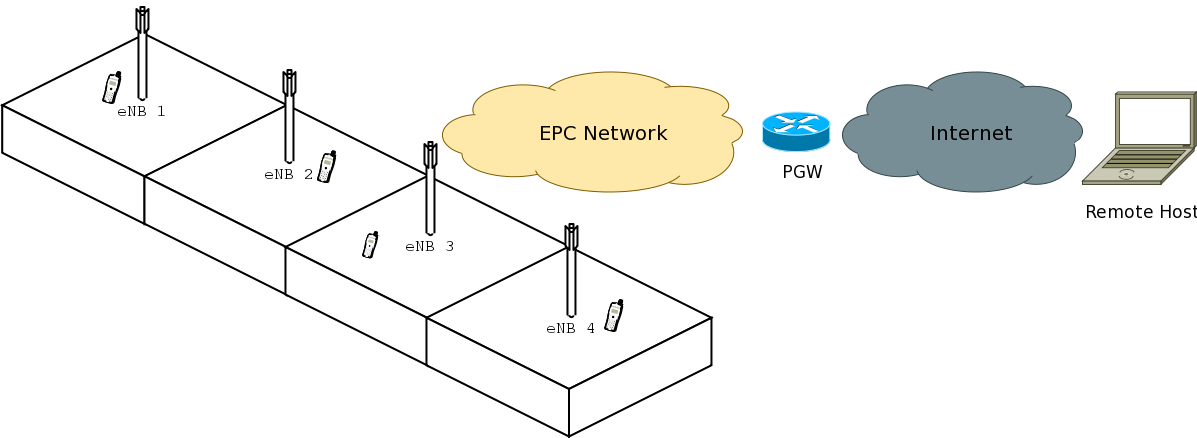
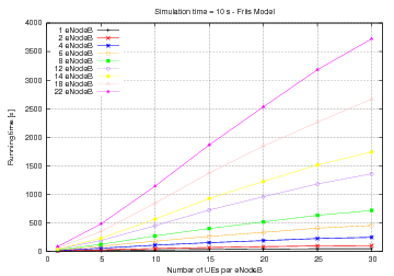
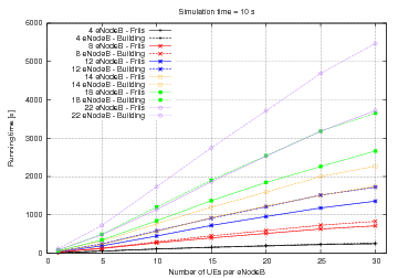
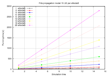
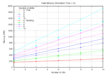
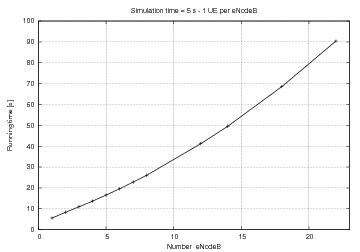
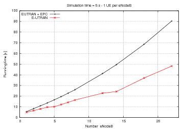
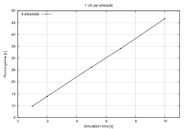
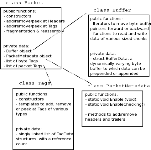
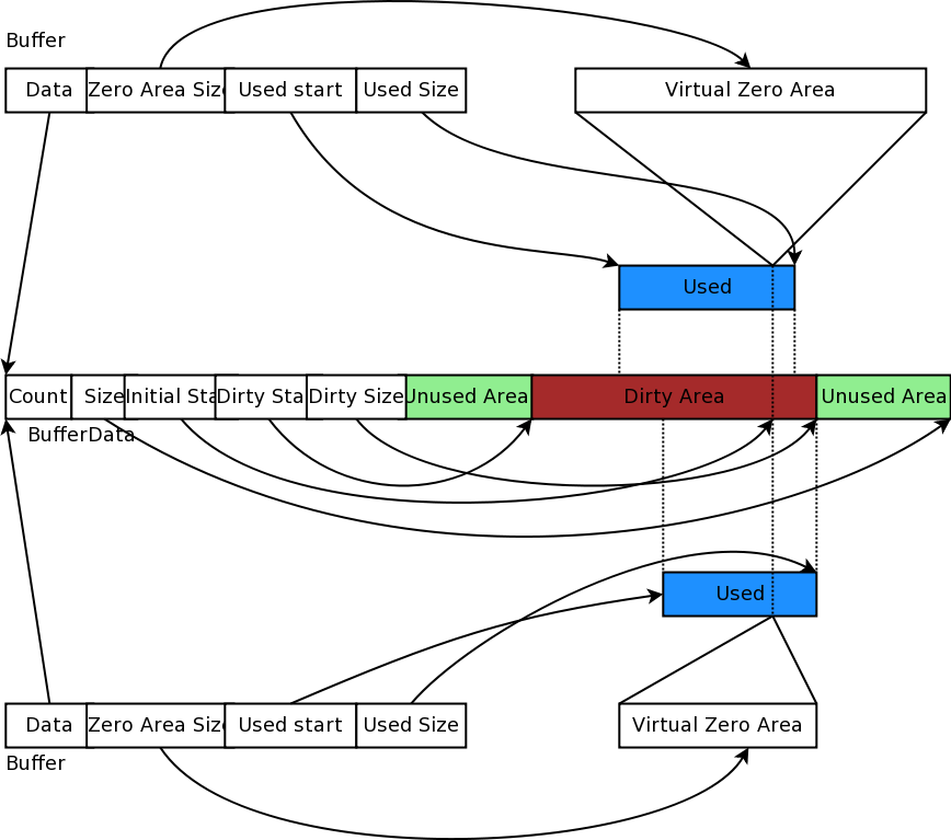
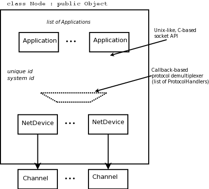
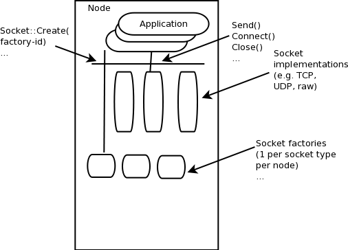


 : transmission power (W)
 : reception power (W)
 : transmission gain (unit-less)
 : reception gain (unit-less)
 : wavelength (m)
 , where
  m/s is the speed of light in
vacuum, and
m/s is the speed of light in
vacuum, and  .
The model will still return a value for
.
The model will still return a value for  , and results in
 for
for  .
. ;
so if, for
;
so if, for  , until
MinLoss is reached, and then stay constant; this allow to
return a value for
, until
MinLoss is reached, and then stay constant; this allow to
return a value for  for
for  .
We note that this value of
.
We note that this value of 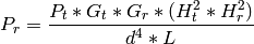
 .
To be consistent with the free space equation,
.
To be consistent with the free space equation,  and
and  are set at the respective nodes
  coordinate plus a model parameter
set via SetHeightAboveZ.
coordinate plus a model parameter
set via SetHeightAboveZ.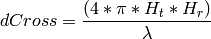
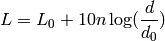
 : reference distance (m)
 : path loss at reference distance (dB)
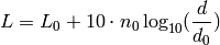

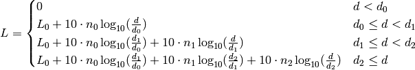
 : three distance fields (m)
 : path loss distance exponent for each field (unitless)
 the average received power.
 the Nakagami-m distribution equals the Rayleigh distribution. Thus
this model also implements Rayleigh distribution based fast fading.
the Nakagami-m distribution equals the Rayleigh distribution. Thus
this model also implements Rayleigh distribution based fast fading.

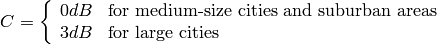
 : eNB height above the ground [m]
 : UE height above the ground [m]
 : is a logarithm in base 10 (this for the whole document)

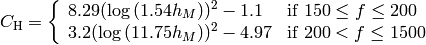
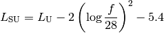
 : pathloss in urban areas
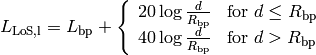
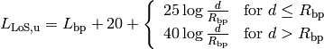
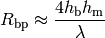
 : UE height above the ground [m]
 is the value for the basic transmission loss at the break point, defined as:
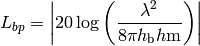
 ), the diffraction loss from rooftop to
street (
), the diffraction loss from rooftop to
street ( ) and the reduction due to multiple screen diffraction past
rows of building (
) and the reduction due to multiple screen diffraction past
rows of building ( ). The formula is:
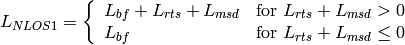

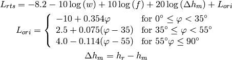
 : is the height of the rooftop [m]
 : is the height of the mobile [m]
 : is the street orientation with respect to the direct path (degrees)

 (where l is the distance over which the building extend),
it can be evaluated according to
(where l is the distance over which the building extend),
it can be evaluated according to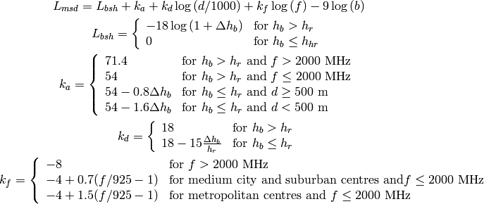
 , the formula is:
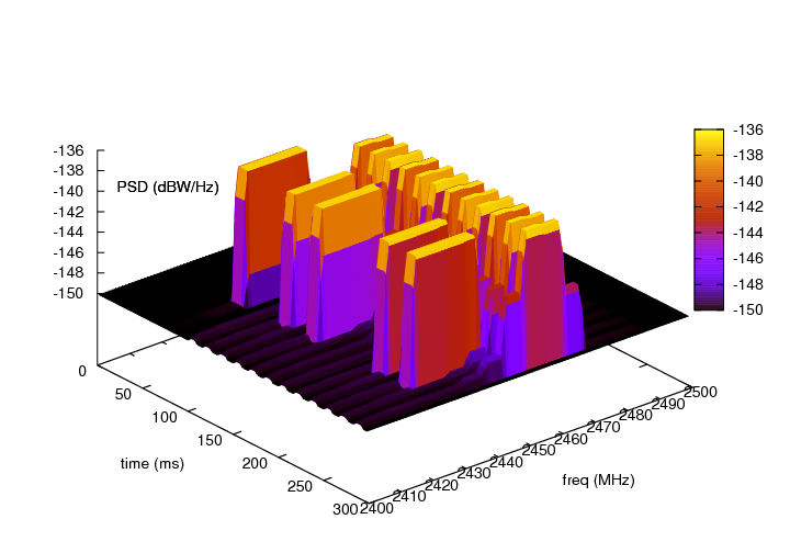
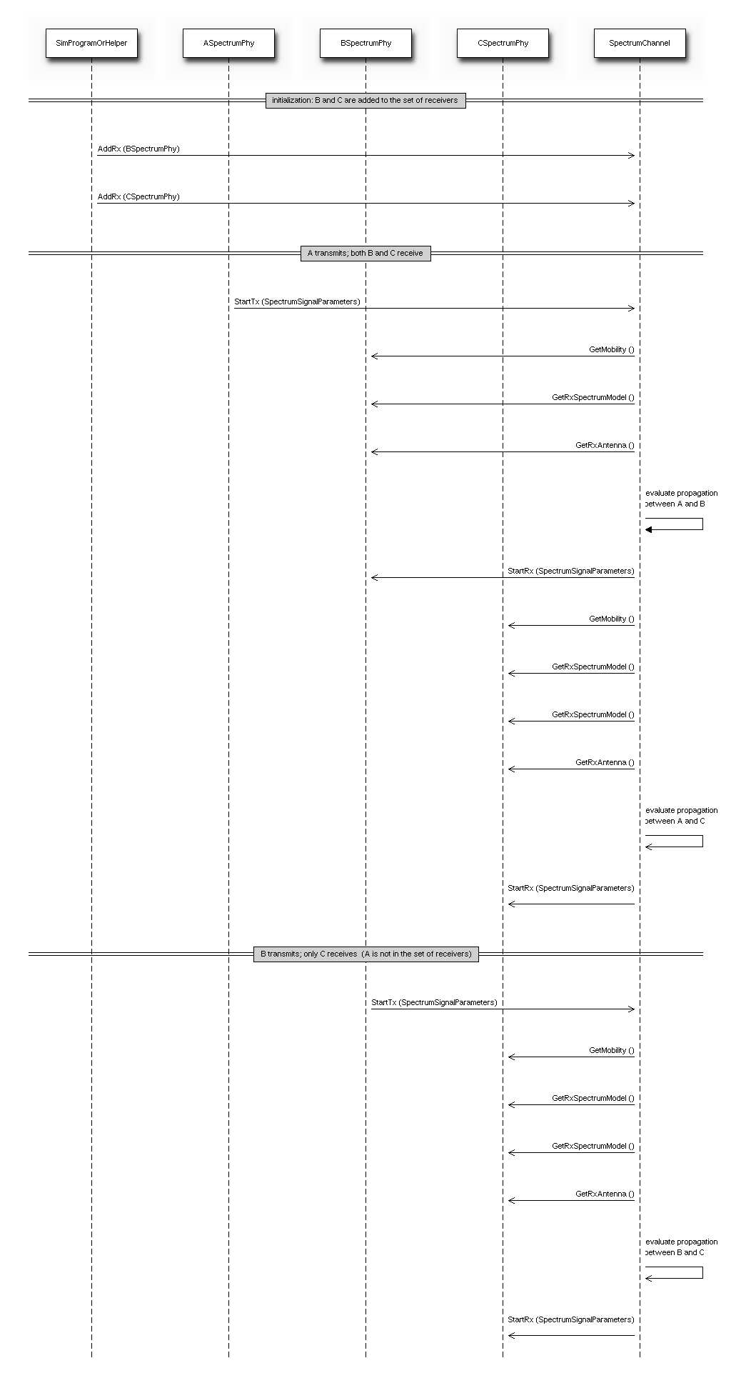
 of the PHY rate;