
Propagation
The ns-3 propagation module defines two generic interfaces, namely PropagationLossModel
and PropagationDelayModel, for the modeling of respectively propagation loss and propagation delay.
PropagationLossModel
Propagation loss models calculate the Rx signal power considering the Tx signal power and the mutual Rx and Tx antennas positions.
A propagation loss model can be “chained” to another one, making a list. The final Rx power takes into account all the chained models. In this way one can use a slow fading and a fast fading model (for example), or model separately different fading effects.
The following propagation loss models are implemented:
- Cost231PropagationLossModel
- FixedRssLossModel
- FriisPropagationLossModel
- ItuR1411LosPropagationLossModel
- ItuR1411NlosOverRooftopPropagationLossModel
- JakesPropagationLossModel
- Kun2600MhzPropagationLossModel
- LogDistancePropagationLossModel
- MatrixPropagationLossModel
- NakagamiPropagationLossModel
- OkumuraHataPropagationLossModel
- RandomPropagationLossModel
- RangePropagationLossModel
- ThreeLogDistancePropagationLossModel
- TwoRayGroundPropagationLossModel
- ThreeGppPropagationLossModel
- ThreeGppRMaPropagationLossModel
- ThreeGppUMaPropagationLossModel
- ThreeGppUmiStreetCanyonPropagationLossModel
- ThreeGppIndoorOfficePropagationLossModel
Other models could be available thanks to other modules, e.g., the building module.
Each of the available propagation loss models of ns-3 is explained in one of the following subsections.
FriisPropagationLossModel
This model implements the Friis propagation loss model. This model was first described in [friis]. The original equation was described as:

with the following equation for the case of an isotropic antenna with no heat loss:

The final equation becomes:

Modern extensions to this original equation are:
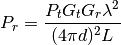
With:
: transmission power (W)
: reception power (W)
: transmission gain (unit-less)
: reception gain (unit-less)
: wavelength (m)
: distance (m)
: system loss (unit-less)
In the implementation, is calculated as
 , where
 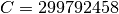 m/s is the speed of light in
vacuum, and
m/s is the speed of light in
vacuum, and  is the frequency in Hz which can be configured by
the user via the Frequency attribute.
is the frequency in Hz which can be configured by
the user via the Frequency attribute.
The Friis model is valid only for propagation in free space within
the so-called far field region, which can be considered
approximately as the region for  .
The model will still return a value for
.
The model will still return a value for  , as
doing so (rather than triggering a fatal error) is practical for
many simulation scenarios. However, we stress that the values
obtained in such conditions shall not be considered realistic.
, as
doing so (rather than triggering a fatal error) is practical for
many simulation scenarios. However, we stress that the values
obtained in such conditions shall not be considered realistic.
Related with this issue, we note that the Friis formula is
undefined for  , and results in
 for
for  .
.
Both these conditions occur outside of the far field region, so in
principle the Friis model shall not be used in these conditions.
In practice, however, Friis is often used in scenarios where accurate
propagation modeling is not deemed important, and values of
can occur.
To allow practical use of the model in such
scenarios, we have to 1) return some value for , and
2) avoid large discontinuities in propagation loss values (which
could lead to artifacts such as bogus capture effects which are
much worse than inaccurate propagation loss values). The two issues
are conflicting, as, according to the Friis formula,
 ;
so if, for , we use a fixed loss value, we end up with an infinitely large
discontinuity, which as we discussed can cause undesirable
simulation artifacts.
;
so if, for , we use a fixed loss value, we end up with an infinitely large
discontinuity, which as we discussed can cause undesirable
simulation artifacts.
To avoid these artifact, this implementation of the Friis model
provides an attribute called MinLoss which allows to specify the
minimum total loss (in dB) returned by the model. This is used in
such a way that
continuously increases for  , until
MinLoss is reached, and then stay constant; this allow to
return a value for and at the same time avoid
discontinuities. The model won’t be much realistic, but at least
the simulation artifacts discussed before are avoided. The default value of
MinLoss is 0 dB, which means that by default the model will return
, until
MinLoss is reached, and then stay constant; this allow to
return a value for and at the same time avoid
discontinuities. The model won’t be much realistic, but at least
the simulation artifacts discussed before are avoided. The default value of
MinLoss is 0 dB, which means that by default the model will return
 for
for 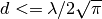 .
We note that this value of is outside of the far field
region, hence the validity of the model in the far field region is
not affected.
.
We note that this value of is outside of the far field
region, hence the validity of the model in the far field region is
not affected.
TwoRayGroundPropagationLossModel
This model implements a Two-Ray Ground propagation loss model ported from NS2
The Two-ray ground reflection model uses the formula
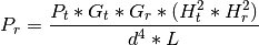
The original equation in Rappaport’s book assumes  .
To be consistent with the free space equation, is added here.
.
To be consistent with the free space equation, is added here.
 and
and  are set at the respective nodes
  coordinate plus a model parameter
set via SetHeightAboveZ.
coordinate plus a model parameter
set via SetHeightAboveZ.
The two-ray model does not give a good result for short distances, due to the oscillation caused by constructive and destructive combination of the two rays. Instead the Friis free-space model is used for small distances.
The crossover distance, below which Friis is used, is calculated as follows:
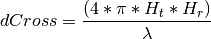
In the implementation, is calculated as
, where m/s is the speed of light in
vacuum, and is the frequency in Hz which can be configured by
the user via the Frequency attribute.
LogDistancePropagationLossModel
This model implements a log distance propagation model.
The reception power is calculated with a so-called log-distance propagation model:
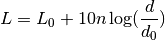
where:
: the path loss distance exponent
: reference distance (m)
: path loss at reference distance (dB)
When the path loss is requested at a distance smaller than the reference distance, the tx power is returned.
ThreeLogDistancePropagationLossModel
This model implements a log distance path loss propagation model with three distance fields. This model is the same as ns3::LogDistancePropagationLossModel except that it has three distance fields: near, middle and far with different exponents.
Within each field the reception power is calculated using the log-distance propagation equation:
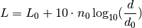
Each field begins where the previous ends and all together form a continuous function.
There are three valid distance fields: near, middle, far. Actually four: the first from 0 to the reference distance is invalid and returns txPowerDbm.

Complete formula for the path loss in dB:
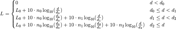
where:
: three distance fields (m)
: path loss distance exponent for each field (unitless)
When the path loss is requested at a distance smaller than the reference
distance , the tx power (with no path loss) is returned. The
reference distance defaults to 1m and reference loss defaults to
FriisPropagationLossModel with 5.15 GHz and is thus = 46.67 dB.
RandomPropagationLossModel
The propagation loss is totally random, and it changes each time the model is called. As a consequence, all the packets (even those between two fixed nodes) experience a random propagation loss.
NakagamiPropagationLossModel
This propagation loss model implements the Nakagami-m fast fading model, which accounts for the variations in signal strength due to multipath fading. The model does not account for the path loss due to the distance traveled by the signal, hence for typical simulation usage it is recommended to consider using it in combination with other models that take into account this aspect.
The Nakagami-m distribution is applied to the power level. The probability density function is defined as
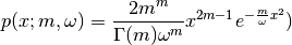
with  the fading depth parameter and
  the average received power.
It is implemented by either a GammaRandomVariable or a ErlangRandomVariable
random variable.
The implementation of the model allows to specify different values of
the parameter (and hence different fast fading profiles)
for three different distance ranges:

For  the Nakagami-m distribution equals the Rayleigh distribution. Thus
this model also implements Rayleigh distribution based fast fading.
the Nakagami-m distribution equals the Rayleigh distribution. Thus
this model also implements Rayleigh distribution based fast fading.
FixedRssLossModel
This model sets a constant received power level independent of the transmit power.
The received power is constant independent of the transmit power; the user must set received power level. Note that if this loss model is chained to other loss models, it should be the first loss model in the chain. Else it will disregard the losses computed by loss models that precede it in the chain.
MatrixPropagationLossModel
The propagation loss is fixed for each pair of nodes and doesn’t depend on their actual positions. This model should be useful for synthetic tests. Note that by default the propagation loss is assumed to be symmetric.
RangePropagationLossModel
This propagation loss depends only on the distance (range) between transmitter and receiver.
The single MaxRange attribute (units of meters) determines path loss. Receivers at or within MaxRange meters receive the transmission at the transmit power level. Receivers beyond MaxRange receive at power -1000 dBm (effectively zero).
OkumuraHataPropagationLossModel
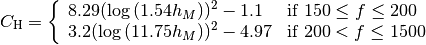
This model is used to model open area pathloss for long distance (i.e., > 1 Km). In order to include all the possible frequencies usable by LTE we need to consider several variants of the well known Okumura Hata model. In fact, the original Okumura Hata model [hata] is designed for frequencies ranging from 150 MHz to 1500 MHz, the COST231 [cost231] extends it for the frequency range from 1500 MHz to 2000 MHz. Another important aspect is the scenarios considered by the models, in fact the all models are originally designed for urban scenario and then only the standard one and the COST231 are extended to suburban, while only the standard one has been extended to open areas. Therefore, the model cannot cover all scenarios at all frequencies. In the following we detail the models adopted.
The pathloss expression of the COST231 OH is:

where

and
: eNB height above the ground [m]
: UE height above the ground [m]
: is a logarithm in base 10 (this for the whole document)
This model is only for urban scenarios.
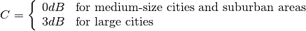
The pathloss expression of the standard OH in urban area is:

where for small or medium sized city

and for large cities
There extension for the standard OH in suburban is
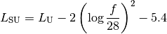
where
: pathloss in urban areas
The extension for the standard OH in open area is

The literature lacks of extensions of the COST231 to open area (for suburban it seems that we can just impose C = 0); therefore we consider it a special case fo the suburban one.
ItuR1411LosPropagationLossModel
This model is designed for Line-of-Sight (LoS) short range outdoor communication in the frequency range 300 MHz to 100 GHz. This model provides an upper and lower bound respectively according to the following formulas
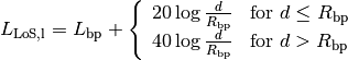
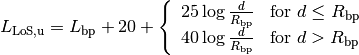
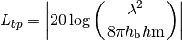
where the breakpoint distance is given by
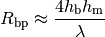
and the above parameters are
: UE height above the ground [m]
and  is the value for the basic transmission loss at the break point, defined as:
The value used by the simulator is the average one for modeling the median pathloss.
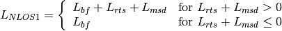
ItuR1411NlosOverRooftopPropagationLossModel
This model is designed for Non-Line-of-Sight (LoS) short range outdoor communication over rooftops in the frequency range 300 MHz to 100 GHz. This model includes several scenario-dependent parameters, such as average street width, orientation, etc. It is advised to set the values of these parameters manually (using the ns-3 attribute system) according to the desired scenario.
In detail, the model is based on [walfisch] and [ikegami], where the loss is expressed
as the sum of free-space loss ( ), the diffraction loss from rooftop to
street (
), the diffraction loss from rooftop to
street ( ) and the reduction due to multiple screen diffraction past
rows of building (
) and the reduction due to multiple screen diffraction past
rows of building ( ). The formula is:
The free-space loss is given by:

where:
) [m]
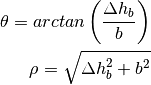
The term takes into account the width of the street and its orientation, according to the formulas
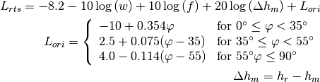
where:
: is the height of the rooftop [m]
: is the height of the mobile [m]
: is the street orientation with respect to the direct path (degrees)
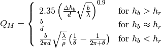
The multiple screen diffraction loss depends on the BS antenna height relative to the building height and on the incidence angle. The former is selected as the higher antenna in the communication link. Regarding the latter, the “settled field distance” is used for select the proper model; its value is given by

with

Therefore, in case of  (where l is the distance over which the building extend),
it can be evaluated according to
(where l is the distance over which the building extend),
it can be evaluated according to
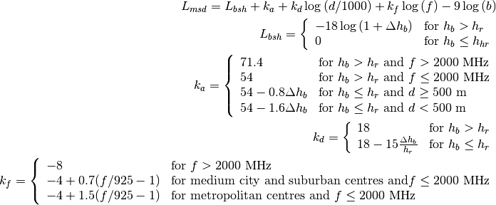
Alternatively, in case of  , the formula is:
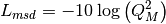
where
where:
Kun2600MhzPropagationLossModel
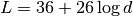
This is the empirical model for the pathloss at 2600 MHz for urban areas which is described in [kun2600mhz].
The model is as follows. Let be the distance between the transmitter and the receiver
in meters; the pathloss in dB is calculated as:
ThreeGppPropagationLossModel
The base class ThreeGppPropagationLossModel and its derived classes implement
the path loss and shadow fading models described in 3GPP TR 38.901 [38901].
3GPP TR 38.901 includes multiple scenarios modeling different propagation
environments, i.e., indoor, outdoor urban and rural, for frequencies between
0.5 and 100 GHz.
Implemented features:
- Path loss and shadowing models (3GPP TR 38.901, Sec. 7.4.1)
- Autocorrelation of shadow fading (3GPP TR 38.901, Sec. 7.4.4)
- Channel condition models (3GPP TR 38.901, Sec. 7.4.2)
To be implemented:
- O2I penetration loss (3GPP TR 38.901, Sec. 7.4.3)
- Spatial consistent update of the channel states (3GPP TR 38.901 Sec. 7.6.3.3)
Configuration
The ThreeGppPropagationLossModel instance is paired with a ChannelConditionModel
instance used to retrieve the LOS/NLOS channel condition. By default, a 3GPP
channel condition model related to the same scenario is set (e.g., by default,
ThreeGppRmaPropagationLossModel is paired with
ThreeGppRmaChannelConditionModel), but it can be configured using
the method SetChannelConditionModel. The channel condition models are stored inside the
propagation module, for a limitation of the current spectrum API and to avoid
a circular dependency between the spectrum and the propagation modules. Please
note that it is necessary to install at least one ChannelConditionModel when
using any ThreeGppPropagationLossModel subclass. Please look below for more
information about the Channel Condition models.
The operating frequency has to be set using the attribute “Frequency”, otherwise an assert is raised. The addition of the shadow fading component can be enabled/disabled through the attribute “ShadowingEnabled”. Other scenario-related parameters can be configured through attributes of the derived classes.
Implementation details
The method DoCalcRxPower computes the propagation loss considering the path loss and the shadow fading (if enabled). The path loss is computed by the method GetLossLos or GetLossNlos depending on the LOS/NLOS channel condition, and their implementation is left to the derived classes. The shadow fading is computed by the method GetShadowing, which generates an additional random loss component characterized by Gaussian distribution with zero mean and scenario-specific standard deviation. Subsequent shadowing components of each BS-UT link are correlated as described in 3GPP TR 38.901, Sec. 7.4.4 [38901].
Note 1: The TR defines height ranges for UTs and BSs, depending on the chosen propagation model (for the exact values, please see below in the specific model documentation). If the user does not set correct values, the model will emit a warning but perform the calculation anyway.
Note 2: The 3GPP model is originally intended to be used to represent BS-UT links. However, in ns-3, we may need to compute the pathloss between two BSs or UTs to evaluate the interference. We have decided to support this case by considering the tallest node as a BS and the smallest as a UT. As a consequence, the height values may be outside the validity range of the chosen class: therefore, an inaccuracy warning may be printed, but it can be ignored.
There are four derived class, each one implementing the propagation model for a different scenario:
ThreeGppRMaPropagationLossModel
This class implements the LOS/NLOS path loss and shadow fading models described in 3GPP TR 38.901 [38901], Table 7.4.1-1 for the RMa scenario. It supports frequencies between 0.5 and 30 GHz. It is possible to configure some scenario-related parameters through the attributes AvgBuildingHeight and AvgStreetWidth.
As specified in the TR, the 2D distance between the transmitter and the receiver should be between 10 m and 10 km for the LOS case, or between 10 m and 5 km for the NLOS case, otherwise the model may not be accurate (a warning message is printed if the user has enabled logging on the model). Also, the height of the base station (hBS) should be between 10 m and 150 m, while the height of the user terminal (hUT) should be between 1 m and 10 m.
ThreeGppUMaPropagationLossModel
This implements the LOS/NLOS path loss and shadow fading models described in 3GPP TR 38.901 [38901], Table 7.4.1-1 for the UMa scenario. It supports frequencies between 0.5 and 100 GHz.
As specified in the TR, the 2D distance between the transmitter and the receiver should be between 10 m and 5 km both for the LOS and NLOS cases, otherwise the model may not be accurate (a warning message is printed if the user has enabled logging on the model). Also, the height of the base station (hBS) should be 25 m and the height of the user terminal (hUT) should be between 1.5 m and 22.5 m.
ThreeGppUmiStreetCanyonPropagationLossModel
This implements the LOS/NLOS path loss and shadow fading models described in 3GPP TR 38.901 [38901], Table 7.4.1-1 for the UMi-Street Canyon scenario. It supports frequencies between 0.5 and 100 GHz.
As specified in the TR, the 2D distance between the transmitter and the receiver should be between 10 m and 5 km both for the LOS and NLOS cases, otherwise the model may not be accurate (a warning message is printed if the user has enabled logging on the model). Also, the height of the base station (hBS) should be 10 m and the height of the user terminal (hUT) should be between 1.5 m and 10 m (the validity range is reduced because we assume that the height of the UT nodes is always lower that the height of the BS nodes).
ThreeGppIndoorOfficePropagationLossModel
This implements the LOS/NLOS path loss and shadow fading models described in 3GPP TR 38.901 [38901], Table 7.4.1-1 for the Indoor-Office scenario. It supports frequencies between 0.5 and 100 GHz.
As specified in the TR, the 3D distance between the transmitter and the receiver should be between 1 m and 150 m both for the LOS and NLOS cases, otherwise the model may not be accurate (a warning log message is printed if the user has enabled logging on the model).
Testing
The test suite ThreeGppPropagationLossModelsTestSuite provides test cases for the classes
implementing the 3GPP propagation loss models.
The test cases ThreeGppRmaPropagationLossModelTestCase,
ThreeGppUmaPropagationLossModelTestCase,
ThreeGppUmiPropagationLossModelTestCase and
ThreeGppIndoorOfficePropagationLossModelTestCase compute the path loss between two nodes and compares it with the value obtained using the formulas in 3GPP TR 38.901 [38901], Table 7.4.1-1.
The test case ThreeGppShadowingTestCase checks if the shadowing is correctly computed by testing the deviation of the overall propagation loss from the path loss. The test is carried out for all the scenarios, both in LOS and NLOS condition.
ChannelConditionModel
The loss models require to know if two nodes are in Line-of-Sight (LoS) or if
they are not. The interface for that is represented by this class. The main
method is GetChannelCondition (a, b), which returns a ChannelCondition object
containing the information about the channel state.
We modeled the LoS condition in two ways: (i) by using a probabilistic model specified by the 3GPP (), and (ii) by using an ns-3 specific building-aware model, which checks the space position of the BSs and the UTs. For what regards the first option, the probability is independent of the node location: in other words, following the 3GPP model, two UT spatially separated by an epsilon may have different LoS conditions. To take into account mobility, we have inserted a parameter called “UpdatePeriod,” which indicates how often a 3GPP-based channel condition has to be updated. By default, this attribute is set to 0, meaning that after the channel condition is generated, it is never updated. With this default value, we encourage the users to run multiple simulations with different seeds to get statistical significance from the data. For the users interested in using mobile nodes, we suggest changing this parameter to a value that takes into account the node speed and the desired accuracy. For example, lower-speed node conditions may be updated in terms of seconds, while high-speed UT or BS may be updated more often.
The two approach are coded, respectively, in the classes:
ThreeGppChannelConditionModelBuildingsChannelConditionModel(see thebuildingmodule documentation for further details)
ThreeGppChannelConditionModel
This is the base class for the 3GPP channel condition models. It provides the possibility to updated the condition of each channel periodically, after a given time period which can be configured through the attribute “UpdatePeriod”. If “UpdatePeriod” is set to 0, the channel condition is never updated. It has five derived classes implementing the channel condition models described in 3GPP TR 38.901 [38901] for different propagation scenarios.
ThreeGppRmaChannelConditionModel
This implements the statistical channel condition model described in 3GPP TR 38.901 [38901], Table 7.4.2-1, for the RMa scenario.
ThreeGppUmaChannelConditionModel
This implements the statistical channel condition model described in 3GPP TR 38.901 [38901], Table 7.4.2-1, for the UMa scenario.
ThreeGppUmiStreetCanyonChannelConditionModel
This implements the statistical channel condition model described in 3GPP TR 38.901 [38901], Table 7.4.2-1, for the UMi-Street Canyon scenario.
Testing
The test suite ChannelConditionModelsTestSuite contains a single test case:
ThreeGppChannelConditionModelTestCase, which tests all the 3GPP channel condition models. It determines the channel condition between two nodes multiple times, estimates the LOS probability, and compares it with the value given by the formulas in 3GPP TR 38.901 [38901], Table 7.4.2-1
PropagationDelayModel
The following propagation delay models are implemented:
- ConstantSpeedPropagationDelayModel
- RandomPropagationDelayModel
ConstantSpeedPropagationDelayModel
In this model, the signal travels with constant speed. The delay is calculated according with the transmitter and receiver positions. The Euclidean distance between the Tx and Rx antennas is used. Beware that, according to this model, the Earth is flat.
RandomPropagationDelayModel
The propagation delay is totally random, and it changes each time the model is called. All the packets (even those between two fixed nodes) experience a random delay. As a consequence, the packets order is not preserved.
References
| [friis] | Friis, H.T., “A Note on a Simple Transmission Formula,” Proceedings of the IRE , vol.34, no.5, pp.254,256, May 1946 |
| [hata] | M.Hata, “Empirical formula for propagation loss in land mobile radio services”, IEEE Trans. on Vehicular Technology, vol. 29, pp. 317-325, 1980 |
| [cost231] | “Digital Mobile Radio: COST 231 View on the Evolution Towards 3rd Generation Systems”, Commission of the European Communities, L-2920, Luxembourg, 1989 |
| [walfisch] | J.Walfisch and H.L. Bertoni, “A Theoretical model of UHF propagation in urban environments,” in IEEE Trans. Antennas Propagat., vol.36, 1988, pp.1788- 1796 |
| [ikegami] | F.Ikegami, T.Takeuchi, and S.Yoshida, “Theoretical prediction of mean field strength for Urban Mobile Radio”, in IEEE Trans. Antennas Propagat., Vol.39, No.3, 1991 |
| [kun2600mhz] | Sun Kun, Wang Ping, Li Yingze, “Path loss models for suburban scenario at 2.3GHz, 2.6GHz and 3.5GHz”, in Proc. of the 8th International Symposium on Antennas, Propagation and EM Theory (ISAPE), Kunming, China, Nov 2008. |
| [38901] | (1, 2, 3, 4, 5, 6, 7, 8, 9, 10, 11, 12, 13, 14) 3GPP. 2018. TR 38.901, Study on channel model for frequencies from 0.5 to 100 GHz, V15.0.0. (2018-06). |