
ns-3 Model Library
This is the ns-3 Model Library documentation. Primary documentation for the ns-3 project is available in five forms:
- ns-3 Doxygen: Documentation of the public APIs of the simulator
- Tutorial, Manual, and Model Library (this document) for the latest release and development tree
- ns-3 wiki
This document is written in reStructuredText for Sphinx and is maintained in the
doc/models directory of ns-3’s source code.
Organization
This manual compiles documentation for ns-3 models and supporting software that enable users to construct network simulations. It is important to distinguish between modules and models:
- ns-3 software is organized into separate modules that are each built as a separate software library. Individual ns-3 programs can link the modules (libraries) they need to conduct their simulation.
- ns-3 models are abstract representations of real-world objects, protocols, devices, etc.
An ns-3 module may consist of more than one model (for instance, the
internet module contains models for both TCP and UDP). In general,
ns-3 models do not span multiple software modules, however.
This manual provides documentation about the models of ns-3. It complements two other sources of documentation concerning models:
- the model APIs are documented, from a programming perspective, using Doxygen. Doxygen for ns-3 models is available on the project web server.
- the ns-3 core is documented in the developer’s manual. ns-3 models make use of the facilities of the core, such as attributes, default values, random numbers, test frameworks, etc. Consult the main web site to find copies of the manual.
Finally, additional documentation about various aspects of ns-3 may exist on the project wiki.
A sample outline of how to write model library documentation can be
found by executing the create-module.py program and looking at the
template created in the file new-module/doc/new-module.rst.
$ cd src
$ ./create-module.py new-module
The remainder of this document is organized alphabetically by module name.
If you are new to ns-3, you might first want to read below about the network module, which contains some fundamental models for the simulator. The packet model, models for different address formats, and abstract base classes for objects such as nodes, net devices, channels, sockets, and applications are discussed there.
Animation
Animation is an important tool for network simulation. While ns-3 does not contain a default graphical animation tool, we currently have two ways to provide animation, namely using the PyViz method or the NetAnim method. The PyViz method is described in http://www.nsnam.org/wiki/PyViz.
We will describe the NetAnim method briefly here.
NetAnim
NetAnim is a standalone, Qt4-based software executable that uses a trace file generated during an ns-3 simulation to display the topology and animate the packet flow between nodes.
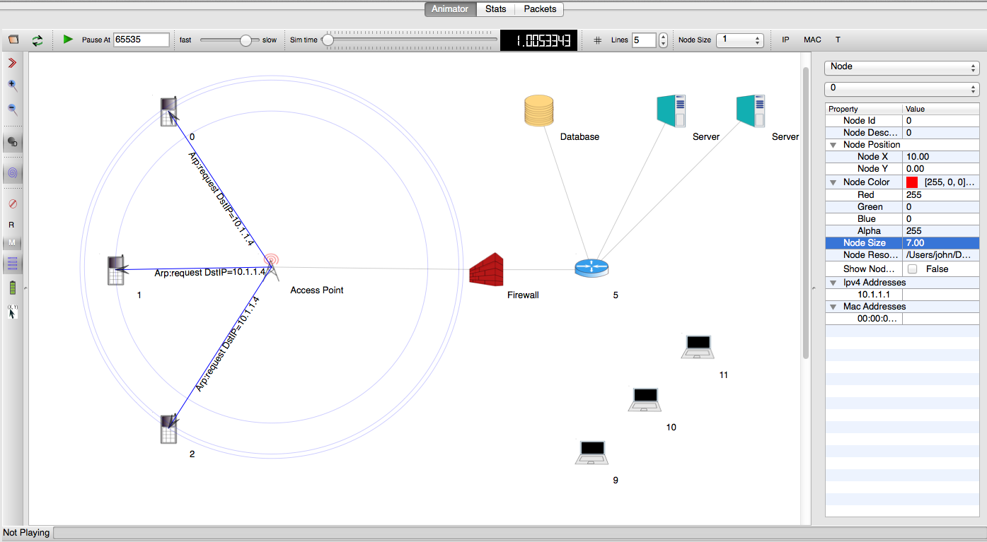
An example of packet animation on wired-links
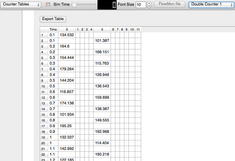
In addition, NetAnim also provides useful features such as tables to display meta-data of packets like the image below
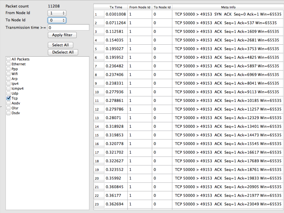
An example of tables for packet meta-data with protocol filters
A way to visualize the trajectory of a mobile node
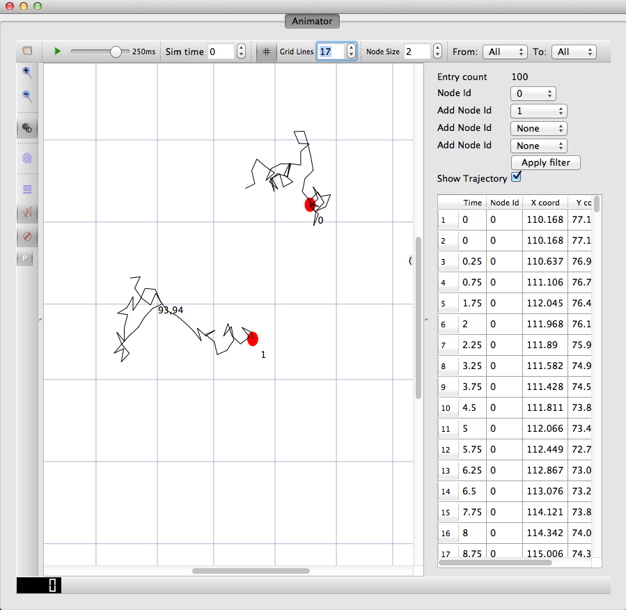
An example of the trajectory of a mobile node
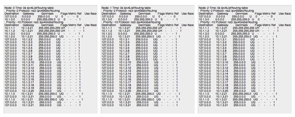
A way to display the routing-tables of multiple nodes at various points in time
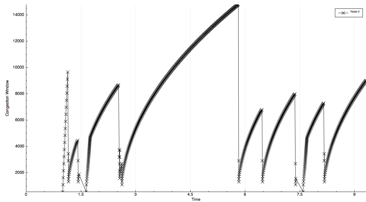
A way to display counters associated with multiple nodes as a chart or a table
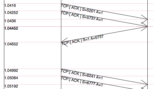
A way to view the timeline of packet transmit and receive events
Methodology
The class ns3::AnimationInterface is responsible for the creation the trace XML file. AnimationInterface uses the tracing infrastructure to track packet flows between nodes. AnimationInterface registers itself as a trace hook for tx and rx events before the simulation begins. When a packet is scheduled for transmission or reception, the corresponding tx and rx trace hooks in AnimationInterface are called. When the rx hooks are called, AnimationInterface will be aware of the two endpoints between which a packet has flowed, and adds this information to the trace file, in XML format along with the corresponding tx and rx timestamps. The XML format will be discussed in a later section. It is important to note that AnimationInterface records a packet only if the rx trace hooks are called. Every tx event must be matched by an rx event.
Downloading NetAnim
If NetAnim is not already available in the ns-3 package you downloaded, you can do the following:
Please ensure that you have installed mercurial. The latest version of NetAnim can be downloaded using mercurial with the following command:
$ hg clone http://code.nsnam.org/netanim
Building NetAnim
Prerequisites
Qt5 (5.4 and over) is required to build NetAnim. This can be obtained using the following ways:
For Ubuntu Linux distributions:
$ apt-get install qt5-default
For Red Hat/Fedora based distribution:
$ yum install qt5
$ yum install qt5-devel
For Mac/OSX, see http://qt.nokia.com/downloads/
Build steps
To build NetAnim use the following commands:
$ cd netanim
$ make clean
$ qmake NetAnim.pro
$ make
Note: qmake could be “qmake-qt5” in some systems
This should create an executable named “NetAnim” in the same directory:
 $ ls -l NetAnim
-rwxr-xr-x 1 john john 390395 2012-05-22 08:32 NetAnim
Usage
Using NetAnim is a two-step process
Step 1:Generate the animation XML trace file during simulation using “ns3::AnimationInterface” in the ns-3 code base.
Step 2:Load the XML trace file generated in Step 1 with the offline Qt4-based animator named NetAnim.
Step 1: Generate XML animation trace file
The class “AnimationInterface” under “src/netanim” uses underlying ns-3 trace sources to construct a timestamped ASCII file in XML format.
Examples are found under src/netanim/examples Example:
$ ./waf -d debug configure --enable-examples
$ ./waf --run "dumbbell-animation"
The above will create an XML file dumbbell-animation.xml
Mandatory
- Ensure that your program’s wscript includes the “netanim” module. An example of such a wscript is at src/netanim/examples/wscript.
- Include the header [#include “ns3/netanim-module.h”] in your test program
- Add the statement
AnimationInterface anim ("animation.xml"); // where "animation.xml" is any arbitrary filename
[for versions before ns-3.13 you also have to use the line “anim.SetXMLOutput() to set the XML mode and also use anim.StartAnimation();]
Optional
The following are optional but useful steps:
// Step 1
anim.SetMobilityPollInterval (Seconds (1));
AnimationInterface records the position of all nodes every 250 ms by default. The statement above sets the periodic interval at which AnimationInterface records the position of all nodes. If the nodes are expected to move very little, it is useful to set a high mobility poll interval to avoid large XML files.
// Step 2
anim.SetConstantPosition (Ptr< Node > n, double x, double y);
AnimationInterface requires that the position of all nodes be set. In ns-3 this is done by setting an associated MobilityModel. “SetConstantPosition” is a quick way to set the x-y coordinates of a node which is stationary.
// Step 3
anim.SetStartTime (Seconds(150)); and anim.SetStopTime (Seconds(150));
AnimationInterface can generate large XML files. The above statements restricts the window between which AnimationInterface does tracing. Restricting the window serves to focus only on relevant portions of the simulation and creating manageably small XML files
// Step 4
AnimationInterface anim ("animation.xml", 50000);
Using the above constructor ensures that each animation XML trace file has only 50000 packets. For example, if AnimationInterface captures 150000 packets, using the above constructor splits the capture into 3 files
- animation.xml - containing the packet range 1-50000
- animation.xml-1 - containing the packet range 50001-100000
- animation.xml-2 - containing the packet range 100001-150000
// Step 5
anim.EnablePacketMetadata (true);
With the above statement, AnimationInterface records the meta-data of each packet in the xml trace file. Metadata can be used by NetAnim to provide better statistics and filter, along with providing some brief information about the packet such as TCP sequence number or source & destination IP address during packet animation.
CAUTION: Enabling this feature will result in larger XML trace files. Please do NOT enable this feature when using Wimax links.
// Step 6
anim.UpdateNodeDescription (5, "Access-point");
With the above statement, AnimationInterface assigns the text “Access-point” to node 5.
// Step 7
anim.UpdateNodeSize (6, 1.5, 1.5);
With the above statement, AnimationInterface sets the node size to scale by 1.5. NetAnim automatically scales the graphics view to fit the oboundaries of the topology. This means that NetAnim, can abnormally scale a node’s size too high or too low. Using AnimationInterface::UpdateNodeSize allows you to overwrite the default scaling in NetAnim and use your own custom scale.
// Step 8
anim.UpdateNodeCounter (89, 7, 3.4);
With the above statement, AnimationInterface sets the counter with Id == 89, associated with Node 7 with the value 3.4. The counter with Id 89 is obtained using AnimationInterface::AddNodeCounter. An example usage for this is in src/netanim/examples/resource-counters.cc.
Step 2: Loading the XML in NetAnim
- Assuming NetAnim was built, use the command “./NetAnim” to launch NetAnim. Please review the section “Building NetAnim” if NetAnim is not available.
- When NetAnim is opened, click on the File open button at the top-left corner, select the XML file generated during Step 1.
- Hit the green play button to begin animation.
Here is a video illustrating this http://www.youtube.com/watch?v=tz_hUuNwFDs
Wiki
For detailed instructions on installing “NetAnim”, F.A.Qs and loading the XML trace file (mentioned earlier) using NetAnim please refer: http://www.nsnam.org/wiki/NetAnim
Antenna Module
Design documentation
Overview
The Antenna module provides:
- a class (Angles) and utility functions to deal with angles
- a base class (AntennaModel) that provides an interface for the modeling of the radiation pattern of an antenna;
- a set of classes derived from this base class that each models the radiation pattern of different types of antennas;
- a base class (PhasedArrayModel) that provides a flexible interface for modeling a number of Phase Antenna Array (PAA) models
- a class (UniformPlanarArray) derived from this base class, implementing a Uniform Planar Array (UPA) supporting both rectangular and linear lattices
Angles
The Angles class holds information about an angle in 3D space using spherical coordinates in radian units. Specifically, it uses the azimuth-inclination convention, where
- Inclination is the angle between the zenith direction (positive z-axis) and the desired direction. It is included in the range [0, pi] radians.
- Azimuth is the signed angle measured from the positive x-axis, where a positive direction goes towards the positive y-axis. It is included in the range [-pi, pi) radians.
Multiple constructors are present, supporting the most common ways to encode information on a direction. A static boolean variable allows the user to decide whether angles should be printed in radian or degree units.
A number of angle-related utilities are offered, such as radians/degree conversions, for both scalars and vectors, and angle wrapping.
AntennaModel
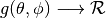
The AntennaModel uses the coordinate system adopted in [Balanis] and
depicted in Figure Coordinate system of the AntennaModel. This system
is obtained by translating the Cartesian coordinate system used by the
ns-3 MobilityModel into the new origin  which is the location
of the antenna, and then transforming the coordinates of every generic
point
which is the location
of the antenna, and then transforming the coordinates of every generic
point  of the space from Cartesian coordinates
 into spherical coordinates
 .
The antenna model neglects the radial component
.
The antenna model neglects the radial component  , and
only considers the angle components
, and
only considers the angle components  . An antenna
radiation pattern is then expressed as a mathematical function
. An antenna
radiation pattern is then expressed as a mathematical function
 that returns the
gain (in dB) for each possible direction of
transmission/reception. All angles are expressed in radians.
that returns the
gain (in dB) for each possible direction of
transmission/reception. All angles are expressed in radians.
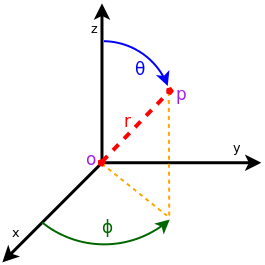
Coordinate system of the AntennaModel
Single antenna models
In this section we describe the antenna radiation pattern models that are included within the antenna module.
IsotropicAntennaModel
This antenna radiation pattern model provides a unitary gain (0 dB) for all direction.
CosineAntennaModel
This is the cosine model described in [Chunjian]: the antenna gain is determined as:
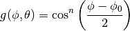
where  is the azimuthal orientation of the antenna
(i.e., its direction of maximum gain) and the exponential
is the azimuthal orientation of the antenna
(i.e., its direction of maximum gain) and the exponential
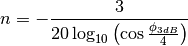
determines the desired 3dB beamwidth  . Note that
this radiation pattern is independent of the inclination angle
. Note that
this radiation pattern is independent of the inclination angle
 .
.
A major difference between the model of [Chunjian] and the one implemented in the class CosineAntennaModel is that only the element factor (i.e., what described by the above formulas) is considered. In fact, [Chunjian] also considered an additional antenna array factor. The reason why the latter is excluded is that we expect that the average user would desire to specify a given beamwidth exactly, without adding an array factor at a latter stage which would in practice alter the effective beamwidth of the resulting radiation pattern.
ParabolicAntennaModel
This model is based on the parabolic approximation of the main lobe radiation pattern. It is often used in the context of cellular system to model the radiation pattern of a cell sector, see for instance [R4-092042a] and [Calcev]. The antenna gain in dB is determined as:
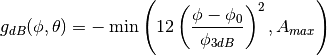
where is the azimuthal orientation of the antenna
(i.e., its direction of maximum gain), is its 3 dB
beamwidth, and  is the maximum attenuation in dB of the
antenna. Note that this radiation pattern is independent of the inclination angle
.
is the maximum attenuation in dB of the
antenna. Note that this radiation pattern is independent of the inclination angle
.
ThreeGppAntennaModel
This model implements the antenna element described in [38901]. Parameters are fixed from the technical report, thus no attributes nor setters are provided. The model is largely based on the ParabolicAntennaModel.
Phased Array Model
The class PhasedArrayModel has been created with flexibility in mind. It abstracts the basic idea of a Phased Antenna Array (PAA) by removing any constraint on the position of each element, and instead generalizes the concept of steering and beamforming vectors, solely based on the generalized location of the antenna elements. For details on Phased Array Antennas see for instance [Mailloux].
Derived classes must implement the following functions:
- GetNumberOfElements: returns the number of antenna elements
- GetElementLocation: returns the location of the antenna element with the specified index, normalized with respect to the wavelength
- GetElementFieldPattern: returns the horizontal and vertical components of the antenna element field pattern at the specified direction. Same polarization (configurable) for all antenna elements of the array is considered.
The class PhasedArrayModel also assumes that all antenna elements are equal, a typical key assumption which allows to model the PAA field pattern as the sum of the array factor, given by the geometry of the location of the antenna elements, and the element field pattern. Any class derived from AntennaModel is a valid antenna element for the PhasedArrayModel, allowing for a great flexibility of the framework.
UniformPlanarArray
The class UniformPlanarArray is a generic implementation of Uniform Planar Arrays (UPAs),
supporting rectangular and linear regular lattices.
It loosely follows the implementation described in the 3GPP TR 38.901 [38901],
considering only a single a single panel, i.e., 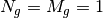 .
.
By default, the array is orthogonal to the x-axis, pointing towards the positive direction, but the orientation can be changed through the attributes “BearingAngle”, which adjusts the azimuth angle, and “DowntiltAngle”, which adjusts the elevation angle. The slant angle is instead fixed and assumed to be 0.
The number of antenna elements in the vertical and horizontal directions can be configured through the attributes “NumRows” and “NumColumns”, while the spacing between the horizontal and vertical elements can be configured through the attributes “AntennaHorizontalSpacing” and “AntennaVerticalSpacing”.
The polarization of each antenna element in the array is determined by the polarization
slant angle through the attribute “PolSlantAngle”, as described in [38901] (i.e.,  ).
).
| [Balanis] | C.A. Balanis, “Antenna Theory - Analysis and Design”, Wiley, 2nd Ed. |
| [Chunjian] | (1, 2, 3) Li Chunjian, “Efficient Antenna Patterns for Three-Sector WCDMA Systems”, Master of Science Thesis, Chalmers University of Technology, Göteborg, Sweden, 2003 |
| [Calcev] | George Calcev and Matt Dillon, “Antenna Tilt Control in CDMA Networks”, in Proc. of the 2nd Annual International Wireless Internet Conference (WICON), 2006 |
| [R4-092042a] | 3GPP TSG RAN WG4 (Radio) Meeting #51, R4-092042, Simulation assumptions and parameters for FDD HeNB RF requirements. |
| [38901] | (1, 2, 3) 3GPP. 2018. TR 38.901, Study on channel model for frequencies from 0.5 to 100 GHz, V15.0.0. (2018-06). |
| [Mailloux] | Robert J. Mailloux, “Phased Array Antenna Handbook”, Artech House, 2nd Ed. |
User Documentation
The antenna modeled can be used with all the wireless technologies and physical layer models that support it. Currently, this includes the physical layer models based on the SpectrumPhy. Please refer to the documentation of each of these models for details.
Testing Documentation
In this section we describe the test suites included with the antenna module that verify its correct functionality.
Angles
The unit test suite angles verifies that the Angles class is
constructed properly by correct conversion from 3D Cartesian
coordinates according to the available methods (construction from a
single vector and from a pair of vectors). For each method, several
test cases are provided that compare the values  determined by the constructor to known reference values. The test
passes if for each case the values are equal to the reference up to a
tolerance of
determined by the constructor to known reference values. The test
passes if for each case the values are equal to the reference up to a
tolerance of  which accounts for numerical errors.
DegreesToRadians
The unit test suite degrees-radians verifies that the methods
DegreesToRadians and RadiansToDegrees work properly by
comparing with known reference values in a number of test
cases. Each test case passes if the comparison is equal up to a
tolerance of which accounts for numerical errors.
IsotropicAntennaModel
The unit test suite isotropic-antenna-model checks that the
IsotropicAntennaModel class works properly, i.e., returns always a
0dB gain regardless of the direction.
CosineAntennaModel
The unit test suite cosine-antenna-model checks that the
CosineAntennaModel class works properly. Several test cases are
provided that check for the antenna gain value calculated at different
directions and for different values of the orientation, the reference
gain and the beamwidth. The reference gain is calculated by hand. Each
test case passes if the reference gain in dB is equal to the value returned
by CosineAntennaModel within a tolerance of 0.001, which accounts
for the approximation done for the calculation of the reference
values.
ParabolicAntennaModel
The unit test suite parabolic-antenna-model checks that the
ParabolicAntennaModel class works properly. Several test cases are
provided that check for the antenna gain value calculated at different
directions and for different values of the orientation, the maximum attenuation
and the beamwidth. The reference gain is calculated by hand. Each
test case passes if the reference gain in dB is equal to the value returned
by ParabolicAntennaModel within a tolerance of 0.001, which accounts
for the approximation done for the calculation of the reference
values.
Ad Hoc On-Demand Distance Vector (AODV)
This model implements the base specification of the Ad Hoc On-Demand Distance Vector (AODV) protocol. The implementation is based on RFC 3561.
The model was written by Elena Buchatskaia and Pavel Boyko of ITTP RAS, and is based on the ns-2 AODV model developed by the CMU/MONARCH group and optimized and tuned by Samir Das and Mahesh Marina, University of Cincinnati, and also on the AODV-UU implementation by Erik Nordström of Uppsala University.
Model Description
The source code for the AODV model lives in the directory src/aodv.
Design
Class ns3::aodv::RoutingProtocol implements all functionality of
service packet exchange and inherits from ns3::Ipv4RoutingProtocol.
The base class defines two virtual functions for packet routing and
forwarding. The first one, ns3::aodv::RouteOutput, is used for
locally originated packets, and the second one, ns3::aodv::RouteInput,
is used for forwarding and/or delivering received packets.
Protocol operation depends on many adjustable parameters. Parameters for
this functionality are attributes of ns3::aodv::RoutingProtocol.
Parameter default values are drawn from the RFC and allow the
enabling/disabling protocol features, such as broadcasting HELLO messages,
broadcasting data packets and so on.
AODV discovers routes on demand. Therefore, the AODV model buffers all
packets while a route request packet (RREQ) is disseminated.
A packet queue is implemented in aodv-rqueue.cc. A smart pointer to
the packet, ns3::Ipv4RoutingProtocol::ErrorCallback,
ns3::Ipv4RoutingProtocol::UnicastForwardCallback, and the IP header
are stored in this queue. The packet queue implements garbage collection
of old packets and a queue size limit.
The routing table implementation supports garbage collection of old entries and state machine, defined in the standard. It is implemented as a STL map container. The key is a destination IP address.
Some elements of protocol operation aren’t described in the RFC. These elements generally concern cooperation of different OSI model layers. The model uses the following heuristics:
- This AODV implementation can detect the presence of unidirectional links and avoid them if necessary. If the node the model receives an RREQ for is a neighbor, the cause may be a unidirectional link. This heuristic is taken from AODV-UU implementation and can be disabled.
- Protocol operation strongly depends on broken link detection mechanism. The model implements two such heuristics. First, this implementation support HELLO messages. However HELLO messages are not a good way to perform neighbor sensing in a wireless environment (at least not over 802.11). Therefore, one may experience bad performance when running over wireless. There are several reasons for this: 1) HELLO messages are broadcasted. In 802.11, broadcasting is often done at a lower bit rate than unicasting, thus HELLO messages can travel further than unicast data. 2) HELLO messages are small, thus less prone to bit errors than data transmissions, and 3) Broadcast transmissions are not guaranteed to be bidirectional, unlike unicast transmissions. Second, we use layer 2 feedback when possible. Link are considered to be broken if frame transmission results in a transmission failure for all retries. This mechanism is meant for active links and works faster than the first method.
The layer 2 feedback implementation relies on the TxErrHeader trace source,
currently supported in AdhocWifiMac only.
Scope and Limitations
The model is for IPv4 only. The following optional protocol optimizations are not implemented:
- Local link repair.
- RREP, RREQ and HELLO message extensions.
These techniques require direct access to IP header, which contradicts the assertion from the AODV RFC that AODV works over UDP. This model uses UDP for simplicity, hindering the ability to implement certain protocol optimizations. The model doesn’t use low layer raw sockets because they are not portable.
Future Work
No announced plans.
3GPP HTTP applications
Model Description
The model is a part of the applications library. The HTTP model is based on a commonly used 3GPP model in standardization [4].
Design
This traffic generator simulates web browsing traffic using the Hypertext
Transfer Protocol (HTTP). It consists of one or more ThreeGppHttpClient
applications which connect to a ThreeGppHttpServer application. The client
models a web browser which requests web pages to the server. The server
is then responsible to serve the web pages as requested. Please refer to
ThreeGppHttpClientHelper and ThreeGppHttpServerHelper for usage instructions.
Technically speaking, the client transmits request objects to demand a service from the server. Depending on the type of request received, the server transmits either:
- a main object, i.e., the HTML file of the web page; or
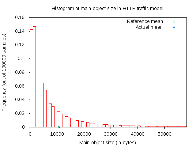
- an embedded object, e.g., an image referenced by the HTML file.
The main and embedded object sizes are illustrated in figures 3GPP HTTP main object size histogram and 3GPP HTTP embedded object size histogram.
3GPP HTTP main object size histogram
3GPP HTTP embedded object size histogram
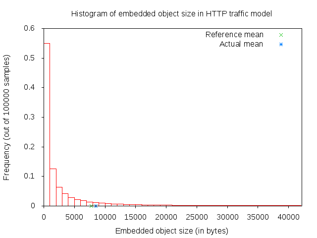
A major portion of the traffic pattern is reading time, which does not generate any traffic. Because of this, one may need to simulate a good number of clients and/or sufficiently long simulation duration in order to generate any significant traffic in the system. Reading time is illustrated in 3GPP HTTP reading time histogram.
3GPP HTTP reading time histogram
3GPP HTTP server description
3GPP HTTP server is a model application which simulates the traffic of a web server. This
application works in conjunction with ThreeGppHttpClient applications.
The application works by responding to requests. Each request is a small
packet of data which contains ThreeGppHttpHeader. The value of the content type
field of the header determines the type of object that the client is
requesting. The possible type is either a main object or an embedded object.
The application is responsible to generate the right type of object and send
it back to the client. The size of each object to be sent is randomly
determined (see ThreeGppHttpVariables). Each object may be sent as multiple packets
due to limited socket buffer space.
To assist with the transmission, the application maintains several instances
of ThreeGppHttpServerTxBuffer. Each instance keeps track of the object type to be
served and the number of bytes left to be sent.
The application accepts connection request from clients. Every connection is kept open until the client disconnects.
Maximum transmission unit (MTU) size is configurable in ThreeGppHttpServer or in
ThreeGppHttpVariables. By default, the low variant is 536 bytes and high variant is 1460 bytes.
The default values are set with the intention of having a TCP header (size of which is 40 bytes) added
in the packet in such way that lower layers can avoid splitting packets. The change of MTU sizes
affects all TCP sockets after the server application has started. It is mainly visible in sizes of
packets received by ThreeGppHttpClient applications.
3GPP HTTP client description
3GPP HTTP client is a model application which simulates the traffic of a web browser. This application works in conjunction with an ThreeGppHttpServer application.
In summary, the application works as follows.
Upon start, it opens a connection to the destination web server (ThreeGppHttpServer).
After the connection is established, the application immediately requests a main object from the server by sending a request packet.
After receiving a main object (which can take some time if it consists of several packets), the application “parses” the main object. Parsing time is illustrated in figure 3GPP HTTP parsing time histogram.
The parsing takes a short time (randomly determined) to determine the number of embedded objects (also randomly determined) in the web page. Number of embedded object is illustrated in 3GPP HTTP number of embedded objects histogram.
- If at least one embedded object is determined, the application requests
- the first embedded object from the server. The request for the next embedded object follows after the previous embedded object has been completely received.
- If there is no more embedded object to request, the application enters
- the reading time.
Reading time is a long delay (again, randomly determined) where the application does not induce any network traffic, thus simulating the user reading the downloaded web page.
After the reading time is finished, the process repeats to step #2.
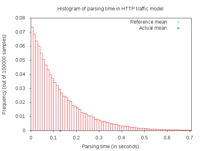
3GPP HTTP parsing time histogram
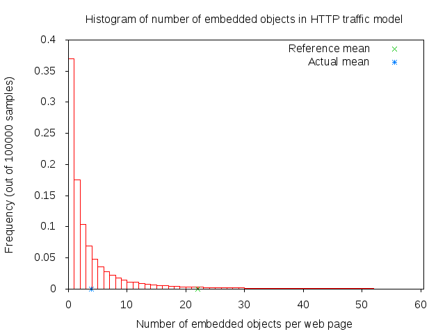
3GPP HTTP number of embedded objects histogram
The client models HTTP persistent connection, i.e., HTTP 1.1, where the connection to the server is maintained and used for transmitting and receiving all objects.
Each request by default has a constant size of 350 bytes. A ThreeGppHttpHeader
is attached to each request packet. The header contains information
such as the content type requested (either main object or embedded object)
and the timestamp when the packet is transmitted (which will be used to
compute the delay and RTT of the packet).
References
Many aspects of the traffic are randomly determined by ThreeGppHttpVariables.
A separate instance of this object is used by the HTTP server and client applications.
These characteristics are based on a legacy 3GPP specification. The description
can be found in the following references:
[1] 3GPP TR 25.892, “Feasibility Study for Orthogonal Frequency Division Multiplexing (OFDM) for UTRAN enhancement”
[2] IEEE 802.16m, “Evaluation Methodology Document (EMD)”, IEEE 802.16m-08/004r5, July 2008.
[3] NGMN Alliance, “NGMN Radio Access Performance Evaluation Methodology”, v1.0, January 2008.
[4] 3GPP2-TSGC5, “HTTP, FTP and TCP models for 1xEV-DV simulations”, 2001.
Usage
The three-gpp-http-example can be referenced to see basic usage of the HTTP applications.
In summary, using the ThreeGppHttpServerHelper and ThreeGppHttpClientHelper allow the
user to easily install ThreeGppHttpServer and ThreeGppHttpClient applications to nodes.
The helper objects can be used to configure attribute values for the client
and server objects, but not for the ThreeGppHttpVariables object. Configuration of variables
is done by modifying attributes of ThreeGppHttpVariables, which should be done prior to helpers
installing applications to nodes.
The client and server provide a number of ns-3 trace sources such as “Tx”, “Rx”, “RxDelay”, and “StateTransition” on the server side, and a large number on the client side (“ConnectionEstablished”, “ConnectionClosed”,”TxMainObjectRequest”, “TxEmbeddedObjectRequest”, “RxMainObjectPacket”, “RxMainObject”, “RxEmbeddedObjectPacket”, “RxEmbeddedObject”, “Rx”, “RxDelay”, “RxRtt”, “StateTransition”).
Building the 3GPP HTTP applications
Building the applications does not require any special steps to be taken. It suffices to enable the applications module.
Examples
For an example demonstrating HTTP applications run:
$ ./waf --run 'three-gpp-http-example'
By default, the example will print out the web page requests of the client and responses of the
server and client receiving content packets by using LOG_INFO of ThreeGppHttpServer and ThreeGppHttpClient.
Tests
For testing HTTP applications, three-gpp-http-client-server-test is provided. Run:
$ ./test.py -s three-gpp-http-client-server-test
The test consists of simple Internet nodes having HTTP server and client applications installed. Multiple variant scenarios are tested: delay is 3ms, 30ms or 300ms, bit error rate 0 or 5.0*10^(-6), MTU size 536 or 1460 bytes and either IPV4 or IPV6 is used. A simulation with each combination of these parameters is run multiple times to verify functionality with different random variables.
Test cases themselves are rather simple: test verifies that HTTP object packet bytes sent match
total bytes received by the client, and that ThreeGppHttpHeader matches the expected packet.
Bridge NetDevice
Placeholder chapter
Some examples of the use of Bridge NetDevice can be found in examples/csma/
directory.
BRITE Integration
This model implements an interface to BRITE, the Boston university Representative Internet Topology gEnerator [1]. BRITE is a standard tool for generating realistic internet topologies. The ns-3 model, described herein, provides a helper class to facilitate generating ns-3 specific topologies using BRITE configuration files. BRITE builds the original graph which is stored as nodes and edges in the ns-3 BriteTopolgyHelper class. In the ns-3 integration of BRITE, the generator generates a topology and then provides access to leaf nodes for each AS generated. ns-3 users can than attach custom topologies to these leaf nodes either by creating them manually or using topology generators provided in ns-3.
There are three major types of topologies available in BRITE: Router, AS, and Hierarchical which is a combination of AS and Router. For the purposes of ns-3 simulation, the most useful are likely to be Router and Hierarchical. Router level topologies be generated using either the Waxman model or the Barabasi-Albert model. Each model has different parameters that effect topology creation. For flat router topologies, all nodes are considered to be in the same AS.
BRITE Hierarchical topologies contain two levels. The first is the AS level. This level can be also be created by using either the Waxman model or the Barabasi-Albert model. Then for each node in the AS topology, a router level topology is constructed. These router level topologies can again either use the Waxman model or the Barbasi-Albert model. BRITE interconnects these separate router topologies as specified by the AS level topology. Once the hierarchical topology is constructed, it is flattened into a large router level topology.
Further information can be found in the BRITE user manual: http://www.cs.bu.edu/brite/publications/usermanual.pdf
Model Description
The model relies on building an external BRITE library,
and then building some ns-3 helpers that call out to the library.
The source code for the ns-3 helpers lives in the directory
src/brite/helper.
Design
To generate the BRITE topology, ns-3 helpers call out to the external BRITE library, and using a standard BRITE configuration file, the BRITE code builds a graph with nodes and edges according to this configuration file. Please see the BRITE documentation or the example configuration files in src/brite/examples/conf_files to get a better grasp of BRITE configuration options. The graph built by BRITE is returned to ns-3, and a ns-3 implementation of the graph is built. Leaf nodes for each AS are available for the user to either attach custom topologies or install ns-3 applications directly.
References
| [1] | Alberto Medina, Anukool Lakhina, Ibrahim Matta, and John Byers. BRITE: An Approach to Universal Topology Generation. In Proceedings of the International Workshop on Modeling, Analysis and Simulation of Computer and Telecommunications Systems- MASCOTS ‘01, Cincinnati, Ohio, August 2001. |
Usage
The brite-generic-example can be referenced to see basic usage of the BRITE interface. In summary, the BriteTopologyHelper is used as the interface point by passing in a BRITE configuration file. Along with the configuration file a BRITE formatted random seed file can also be passed in. If a seed file is not passed in, the helper will create a seed file using ns-3’s UniformRandomVariable. Once the topology has been generated by BRITE, BuildBriteTopology() is called to create the ns-3 representation. Next IP Address can be assigned to the topology using either AssignIpv4Addresses() or AssignIpv6Addresses(). It should be noted that each point-to-point link in the topology will be treated as a new network therefore for IPV4 a /30 subnet should be used to avoid wasting a large amount of the available address space.
Example BRITE configuration files can be found in /src/brite/examples/conf_files/. ASBarbasi and ASWaxman are examples of AS only topologies. The RTBarabasi and RTWaxman files are examples of router only topologies. Finally the TD_ASBarabasi_RTWaxman configuration file is an example of a Hierarchical topology that uses the Barabasi-Albert model for the AS level and the Waxman model for each of the router level topologies. Information on the BRITE parameters used in these files can be found in the BRITE user manual.
Building BRITE Integration
The first step is to download and build the ns-3 specific BRITE repository:
$ hg clone http://code.nsnam.org/BRITE
$ cd BRITE
$ make
This will build BRITE and create a library, libbrite.so, within the BRITE directory.
Once BRITE has been built successfully, we proceed to configure ns-3 with BRITE support. Change to your ns-3 directory:
$ ./waf configure --with-brite=/your/path/to/brite/source --enable-examples
Make sure it says ‘enabled’ beside ‘BRITE Integration’. If it does not, then something has gone wrong. Either you have forgotten to build BRITE first following the steps above, or ns-3 could not find your BRITE directory.
Next, build ns-3:
$ ./waf
Examples
For an example demonstrating BRITE integration run:
$ ./waf --run 'brite-generic-example'
By enabling the verbose parameter, the example will print out the node and edge information in a similar format to standard BRITE output. There are many other command-line parameters including confFile, tracing, and nix, described below:
- confFile
- A BRITE configuration file. Many different BRITE configuration file examples exist in the src/brite/examples/conf_files directory, for example, RTBarabasi20.conf and RTWaxman.conf. Please refer to the conf_files directory for more examples.
- tracing
- Enables ascii tracing.
- nix
- Enables nix-vector routing. Global routing is used by default.
The generic BRITE example also support visualization using pyviz, assuming python bindings in ns-3 are enabled:
$ ./waf --run brite-generic-example --vis
Simulations involving BRITE can also be used with MPI. The total number of MPI instances is passed to the BRITE topology helper where a modulo divide is used to assign the nodes for each AS to a MPI instance. An example can be found in src/brite/examples:
$ mpirun -np 2 ./waf --run brite-MPI-example
Please see the ns-3 MPI documentation for information on setting up MPI with ns-3.
Buildings Module
cd .. include:: replace.txt
Design documentation
Overview
The Buildings module provides:
- a new class (
Building) that models the presence of a building in a simulation scenario;- a new class (
MobilityBuildingInfo) that allows to specify the location, size and characteristics of buildings present in the simulated area, and allows the placement of nodes inside those buildings;- a container class with the definition of the most useful pathloss models and the correspondent variables called
BuildingsPropagationLossModel.- a new propagation model (
HybridBuildingsPropagationLossModel) working with the mobility model just introduced, that allows to model the phenomenon of indoor/outdoor propagation in the presence of buildings.- a simplified model working only with Okumura Hata (
OhBuildingsPropagationLossModel) considering the phenomenon of indoor/outdoor propagation in the presence of buildings.- a channel condition model (
BuildingsChannelConditionModel) which determined the LOS/NLOS channel condition based on theBuildingobjects deployed in the scenario.- hybrid channel condition models (
ThreeGppV2vUrbanChannelConditionModelandThreeGppV2vHighwayChannelConditionModel) specifically designed to model vehicular environments (more information can be found in the documentation of the propagation module)
The models have been designed with LTE in mind, though their implementation is in fact independent from any LTE-specific code, and can be used with other ns-3 wireless technologies as well (e.g., wifi, wimax).
The HybridBuildingsPropagationLossModel pathloss model included is obtained through a combination of several well known pathloss models in order to mimic different environmental scenarios such as urban, suburban and open areas. Moreover, the model considers both outdoor and indoor indoor and outdoor communication has to be included since HeNB might be installed either within building and either outside. In case of indoor communication, the model has to consider also the type of building in outdoor <-> indoor communication according to some general criteria such as the wall penetration losses of the common materials; moreover it includes some general configuration for the internal walls in indoor communications.
The OhBuildingsPropagationLossModel pathloss model has been created for simplifying the previous one removing the thresholds for switching from one model to other. For doing this it has been used only one propagation model from the one available (i.e., the Okumura Hata). The presence of building is still considered in the model; therefore all the considerations of above regarding the building type are still valid. The same consideration can be done for what concern the environmental scenario and frequency since both of them are parameters of the model considered.
The Building class
The model includes a specific class called Building which contains a ns3 Box class for defining the dimension of the building. In order to implements the characteristics of the pathloss models included, the Building class supports the following attributes:
- building type:
- Residential (default value)
- Office
- Commercial
- external walls type
- Wood
- ConcreteWithWindows (default value)
- ConcreteWithoutWindows
- StoneBlocks
- number of floors (default value 1, which means only ground-floor)
- number of rooms in x-axis (default value 1)
- number of rooms in y-axis (default value 1)
The Building class is based on the following assumptions:
- a buildings is represented as a rectangular parallelepiped (i.e., a box)
- the walls are parallel to the x, y, and z axis
- a building is divided into a grid of rooms, identified by the following parameters:
- number of floors
- number of rooms along the x-axis
- number of rooms along the y-axis
- the z axis is the vertical axis, i.e., floor numbers increase for increasing z axis values
- the x and y room indices start from 1 and increase along the x and y axis respectively
- all rooms in a building have equal size
The MobilityBuildingInfo class
The MobilityBuildingInfo class, which inherits from the ns3 class Object, is in charge of maintaining information about the position of a node with respect to building. The information managed by MobilityBuildingInfo is:
- whether the node is indoor or outdoor
- if indoor:
- in which building the node is
- in which room the node is positioned (x, y and floor room indices)
The class MobilityBuildingInfo is used by BuildingsPropagationLossModel class, which inherits from the ns3 class PropagationLossModel and manages the pathloss computation of the single components and their composition according to the nodes’ positions. Moreover, it implements also the shadowing, that is the loss due to obstacles in the main path (i.e., vegetation, buildings, etc.).
It is to be noted that, MobilityBuildingInfo can be used by any other propagation model. However, based on the information at the time of this writing, only the ones defined in the building module are designed for considering the constraints introduced by the buildings.
ItuR1238PropagationLossModel
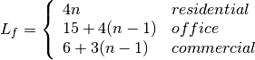
This class implements a building-dependent indoor propagation loss model based on the ITU P.1238 model, which includes losses due to type of building (i.e., residential, office and commercial). The analytical expression is given in the following.
![L_\mathrm{total} = 20\log f + N\log d + L_f(n)- 28 [dB]](_images/math/107e7c14732ab2347fc91e55bd1d30d380de191c.png)
where:
: power loss coefficient [dB]
: number of floors between base station and mobile (
)
: frequency [MHz]
: distance (where
) [m]
BuildingsPropagationLossModel
The BuildingsPropagationLossModel provides an additional set of building-dependent pathloss model elements that are used to implement different pathloss logics. These pathloss model elements are described in the following subsections.
External Wall Loss (EWL)
This component models the penetration loss through walls for indoor to outdoor communications and vice-versa. The values are taken from the [cost231] model.
- Wood ~ 4 dB
- Concrete with windows (not metallized) ~ 7 dB
- Concrete without windows ~ 15 dB (spans between 10 and 20 in COST231)
- Stone blocks ~ 12 dB
Internal Walls Loss (IWL)
This component models the penetration loss occurring in indoor-to-indoor communications within the same building. The total loss is calculated assuming that each single internal wall has a constant penetration loss  , and approximating the number of walls that are penetrated with the manhattan distance (in number of rooms) between the transmitter and the receiver. In detail, let
  ,
,  ,
,  ,
,  denote the room number along the
  and
and  axis respectively for user 1 and 2; the total loss
  is calculated as

Height Gain Model (HG)
This component model the gain due to the fact that the transmitting device is on a floor above the ground. In the literature [turkmani] this gain has been evaluated as about 2 dB per floor. This gain can be applied to all the indoor to outdoor communications and vice-versa.
Shadowing Model
The shadowing is modeled according to a log-normal distribution with variable standard deviation as function of the relative position (indoor or outdoor) of the MobilityModel instances involved. One random value is drawn for each pair of MobilityModels, and stays constant for that pair during the whole simulation. Thus, the model is appropriate for static nodes only.
The model considers that the mean of the shadowing loss in dB is always 0. For the variance, the model considers three possible values of standard deviation, in detail:
- outdoor (
m_shadowingSigmaOutdoor, defaul value of 7 dB).
- indoor (
m_shadowingSigmaIndoor, defaul value of 10 dB).
- external walls penetration (
m_shadowingSigmaExtWalls, default value 5 dB)
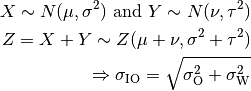
The simulator generates a shadowing value per each active link according to nodes’ position the first time the link is used for transmitting. In case of transmissions from outdoor nodes to indoor ones, and vice-versa, the standard deviation ( ) has to be calculated as the square root of the sum of the quadratic values of the standard deviatio in case of outdoor nodes and the one for the external walls penetration. This is due to the fact that that the components producing the shadowing are independent of each other; therefore, the variance of a distribution resulting from the sum of two independent normal ones is the sum of the variances.
Pathloss logics
In the following we describe the different pathloss logic that are implemented by inheriting from BuildingsPropagationLossModel.
HybridBuildingsPropagationLossModel
The HybridBuildingsPropagationLossModel pathloss model included is obtained through a combination of several well known pathloss models in order to mimic different outdoor and indoor scenarios, as well as indoor-to-outdoor and outdoor-to-indoor scenarios. In detail, the class HybridBuildingsPropagationLossModel integrates the following pathloss models:
- OkumuraHataPropagationLossModel (OH) (at frequencies > 2.3 GHz substituted by Kun2600MhzPropagationLossModel)
- ItuR1411LosPropagationLossModel and ItuR1411NlosOverRooftopPropagationLossModel (I1411)
- ItuR1238PropagationLossModel (I1238)
- the pathloss elements of the BuildingsPropagationLossModel (EWL, HG, IWL)
The following pseudo-code illustrates how the different pathloss model elements described above are integrated in HybridBuildingsPropagationLossModel:
if (txNode is outdoor)
  then
    if (rxNode is outdoor)
      then
        if (distance > 1 km)
          then
            if (rxNode or txNode is below the rooftop)
              then
                L = I1411
              else
                L = OH
          else
            L = I1411
      else (rxNode is indoor)
        if (distance > 1 km)
          then
            if (rxNode or txNode is below the rooftop)
              L = I1411 + EWL + HG
            else
              L = OH + EWL + HG
          else
            L = I1411 + EWL + HG
else (txNode is indoor)
  if (rxNode is indoor)
    then
     if (same building)
        then
          L = I1238 + IWL
        else
          L = I1411 + 2*EWL
   else (rxNode is outdoor)
    if (distance > 1 km)
      then
        if (rxNode or txNode is below the rooftop)
              then
                L = I1411 + EWL + HG
              else
                L = OH + EWL + HG
      else
        L = I1411 + EWL
We note that, for the case of communication between two nodes below rooftop level with distance is greater then 1 km, we still consider the I1411 model, since OH is specifically designed for macro cells and therefore for antennas above the roof-top level.
For the ITU-R P.1411 model we consider both the LOS and NLoS versions. In particular, we considers the LoS propagation for distances that are shorted than a tunable threshold (m_itu1411NlosThreshold). In case on NLoS propagation, the over the roof-top model is taken in consideration for modeling both macro BS and SC. In case on NLoS several parameters scenario dependent have been included, such as average street width, orientation, etc. The values of such parameters have to be properly set according to the scenario implemented, the model does not calculate natively their values. In case any values is provided, the standard ones are used, apart for the height of the mobile and BS, which instead their integrity is tested directly in the code (i.e., they have to be greater then zero). In the following we give the expressions of the components of the model.
We also note that the use of different propagation models (OH, I1411, I1238 with their variants) in HybridBuildingsPropagationLossModel can result in discontinuities of the pathloss with respect to distance. A proper tuning of the attributes (especially the distance threshold attributes) can avoid these discontinuities. However, since the behavior of each model depends on several other parameters (frequency, node height, etc), there is no default value of these thresholds that can avoid the discontinuities in all possible configurations. Hence, an appropriate tuning of these parameters is left to the user.
OhBuildingsPropagationLossModel
The OhBuildingsPropagationLossModel class has been created as a simple means to solve the discontinuity problems of HybridBuildingsPropagationLossModel without doing scenario-specific parameter tuning. The solution is to use only one propagation loss model (i.e., Okumura Hata), while retaining the structure of the pathloss logic for the calculation of other path loss components (such as wall penetration losses). The result is a model that is free of discontinuities (except those due to walls), but that is less realistic overall for a generic scenario with buildings and outdoor/indoor users, e.g., because Okumura Hata is not suitable neither for indoor communications nor for outdoor communications below rooftop level.
In detail, the class OhBuildingsPropagationLossModel integrates the following pathloss models:
- OkumuraHataPropagationLossModel (OH)
- the pathloss elements of the BuildingsPropagationLossModel (EWL, HG, IWL)
The following pseudo-code illustrates how the different pathloss model elements described above are integrated in OhBuildingsPropagationLossModel:
if (txNode is outdoor)
  then
    if (rxNode is outdoor)
      then
        L = OH
      else (rxNode is indoor)
        L = OH + EWL
else (txNode is indoor)
  if (rxNode is indoor)
    then
     if (same building)
        then
          L = OH + IWL
        else
          L = OH + 2*EWL
   else (rxNode is outdoor)
      L = OH + EWL
We note that OhBuildingsPropagationLossModel is a significant simplification with respect to HybridBuildingsPropagationLossModel, due to the fact that OH is used always. While this gives a less accurate model in some scenarios (especially below rooftop and indoor), it effectively avoids the issue of pathloss discontinuities that affects HybridBuildingsPropagationLossModel.
User Documentation
How to use buildings in a simulation
In this section we explain the basic usage of the buildings model within a simulation program.
Include the headers
Add this at the beginning of your simulation program:
#include <ns3/buildings-module.h>
Create a building
As an example, let’s create a residential 10 x 20 x 10 building:
double x_min = 0.0;
double x_max = 10.0;
double y_min = 0.0;
double y_max = 20.0;
double z_min = 0.0;
double z_max = 10.0;
Ptr<Building> b = CreateObject <Building> ();
b->SetBoundaries (Box (x_min, x_max, y_min, y_max, z_min, z_max));
b->SetBuildingType (Building::Residential);
b->SetExtWallsType (Building::ConcreteWithWindows);
b->SetNFloors (3);
b->SetNRoomsX (3);
b->SetNRoomsY (2);
This building has three floors and an internal 3 x 2 grid of rooms of equal size.
The helper class GridBuildingAllocator is also available to easily create a set of buildings with identical characteristics placed on a rectangular grid. Here’s an example of how to use it:
Ptr<GridBuildingAllocator>  gridBuildingAllocator;
gridBuildingAllocator = CreateObject<GridBuildingAllocator> ();
gridBuildingAllocator->SetAttribute ("GridWidth", UintegerValue (3));
gridBuildingAllocator->SetAttribute ("LengthX", DoubleValue (7));
gridBuildingAllocator->SetAttribute ("LengthY", DoubleValue (13));
gridBuildingAllocator->SetAttribute ("DeltaX", DoubleValue (3));
gridBuildingAllocator->SetAttribute ("DeltaY", DoubleValue (3));
gridBuildingAllocator->SetAttribute ("Height", DoubleValue (6));
gridBuildingAllocator->SetBuildingAttribute ("NRoomsX", UintegerValue (2));
gridBuildingAllocator->SetBuildingAttribute ("NRoomsY", UintegerValue (4));
gridBuildingAllocator->SetBuildingAttribute ("NFloors", UintegerValue (2));
gridBuildingAllocator->SetAttribute ("MinX", DoubleValue (0));
gridBuildingAllocator->SetAttribute ("MinY", DoubleValue (0));
gridBuildingAllocator->Create (6);
This will create a 3x2 grid of 6 buildings, each 7 x 13 x 6 m with 2 x 4 rooms inside and 2 foors; the buildings are spaced by 3 m on both the x and the y axis.
Setup nodes and mobility models
Nodes and mobility models are configured as usual, however in order to
use them with the buildings model you need an additional call to
BuildingsHelper::Install(), so as to let the mobility model include
the information on their position w.r.t. the buildings. Here is an example:
MobilityHelper mobility;
mobility.SetMobilityModel ("ns3::ConstantPositionMobilityModel");
ueNodes.Create (2);
mobility.Install (ueNodes);
BuildingsHelper::Install (ueNodes);
It is to be noted that any mobility model can be used. However, the user is advised to make sure that the behavior of the mobility model being used is consistent with the presence of Buildings. For example, using a simple random mobility over the whole simulation area in presence of buildings might easily results in node moving in and out of buildings, regardless of the presence of walls.
One dedicated buildings-aware mobility model is the
RandomWalk2dOutdoorMobilityModel. This class is similar to the
RandomWalk2dMobilityModel but avoids placing the trajectory
on a path that would intersect a building wall. If a boundary
is encountered (either the bounding box or a building wall), the
model rebounds with a random direction and speed that ensures that
the trajectory stays outside the buildings. An example program
that demonstrates the use of this model is the
src/buildings/examples/outdoor-random-walk-example.cc which
has an associated shell script to plot the traces generated.
Another example program demonstrates how this outdoor mobility
model can be used as the basis of a group mobility model, with
the outdoor buildings-aware model serving as the parent or
reference mobility model, and with additional nodes defining a
child mobility model providing the offset from the reference
mobility model. This example,
src/buildings/example/outdoor-group-mobility-example.cc,
also has an associated shell script
(outdoor-group-mobility-animate.sh) that can be used to generate
an animated GIF of the group’s movement.
Place some nodes
You can place nodes in your simulation using several methods, which are described in the following.
Legacy positioning methods
Any legacy ns-3 positioning method can be used to place node in the simulation. The important additional step is to For example, you can place nodes manually like this:
Ptr<ConstantPositionMobilityModel> mm0 = enbNodes.Get (0)->GetObject<ConstantPositionMobilityModel> ();
Ptr<ConstantPositionMobilityModel> mm1 = enbNodes.Get (1)->GetObject<ConstantPositionMobilityModel> ();
mm0->SetPosition (Vector (5.0, 5.0, 1.5));
mm1->SetPosition (Vector (30.0, 40.0, 1.5));

MobilityHelper mobility;
mobility.SetMobilityModel ("ns3::ConstantPositionMobilityModel");
ueNodes.Create (2);
mobility.Install (ueNodes);
BuildingsHelper::Install (ueNodes);
mm0->SetPosition (Vector (5.0, 5.0, 1.5));
mm1->SetPosition (Vector (30.0, 40.0, 1.5));
Alternatively, you could use any existing PositionAllocator class. The coordinates of the node will determine whether it is placed outdoor or indoor and, if indoor, in which building and room it is placed.
Building-specific positioning methods
The following position allocator classes are available to place node in special positions with respect to buildings:
RandomBuildingPositionAllocator: Allocate each position by randomly choosing a building from the list of all buildings, and then randomly choosing a position inside the building.RandomRoomPositionAllocator: Allocate each position by randomly choosing a room from the list of rooms in all buildings, and then randomly choosing a position inside the room.SameRoomPositionAllocator: Walks a given NodeContainer sequentially, and for each node allocate a new position randomly in the same room of that node.FixedRoomPositionAllocator: Generate a random position uniformly distributed in the volume of a chosen room inside a chosen building.
Making the Mobility Model Consistent for a node
Initially, a mobility model of a node is made consistent when a node is
initialized, which eventually triggers a call to the DoInitialize
method of the MobilityBuildingInfo` class. In particular, it calls the
MakeMobilityModelConsistent method, which goes through the lists of
all buildings, determine if the node is indoor or outdoor, and if indoor
it also determines the building in which the node is located and the
corresponding floor number inside the building. Moreover, this method also
caches the position of the node, which is used to make the mobility model
consistent for a moving node whenever the IsInside method of
MobilityBuildingInfo class is called.
Building-aware pathloss model
After you placed buildings and nodes in a simulation, you can use a building-aware pathloss model in a simulation exactly in the same way you would use any regular path loss model. How to do this is specific for the wireless module that you are considering (lte, wifi, wimax, etc.), so please refer to the documentation of that model for specific instructions.
Building-aware channel condition models
The class BuildingsChannelConditionModel implements a channel condition model which determines the LOS/NLOS channel state based on the buildings deployed in the scenario.
The classes ThreeGppV2vUrbanChannelConditionModel and
ThreeGppV2vHighwayChannelConditionModel implement hybrid channel condition
models, specifically designed to model vehicular environments.
More information can be found in the documentation
of the propagation module.
Main configurable attributes
The Building class has the following configurable parameters:
- building type: Residential, Office and Commercial.
- external walls type: Wood, ConcreteWithWindows, ConcreteWithoutWindows and StoneBlocks.
- building bounds: a
Boxclass with the building bounds. - number of floors.
- number of rooms in x-axis and y-axis (rooms can be placed only in a grid way).
The BuildingMobilityLossModel parameter configurable with the ns3 attribute system is represented by the bound (string Bounds) of the simulation area by providing a Box class with the area bounds. Moreover, by means of its methods the following parameters can be configured:
- the number of floor the node is placed (default 0).
- the position in the rooms grid.
The BuildingPropagationLossModel class has the following configurable parameters configurable with the attribute system:
Frequency: reference frequency (default 2160 MHz), note that by setting the frequency the wavelength is set accordingly automatically and viceversa).Lambda: the wavelength (0.139 meters, considering the above frequency).ShadowSigmaOutdoor: the standard deviation of the shadowing for outdoor nodes (defaul 7.0).ShadowSigmaIndoor: the standard deviation of the shadowing for indoor nodes (default 8.0).ShadowSigmaExtWalls: the standard deviation of the shadowing due to external walls penetration for outdoor to indoor communications (default 5.0).RooftopLevel: the level of the rooftop of the building in meters (default 20 meters).Los2NlosThr: the value of distance of the switching point between line-of-sigth and non-line-of-sight propagation model in meters (default 200 meters).ITU1411DistanceThr: the value of distance of the switching point between short range (ITU 1211) communications and long range (Okumura Hata) in meters (default 200 meters).MinDistance: the minimum distance in meters between two nodes for evaluating the pathloss (considered neglictible before this threshold) (default 0.5 meters).Environment: the environment scenario among Urban, SubUrban and OpenAreas (default Urban).CitySize: the dimension of the city among Small, Medium, Large (default Large).
In order to use the hybrid mode, the class to be used is the HybridBuildingMobilityLossModel, which allows the selection of the proper pathloss model according to the pathloss logic presented in the design chapter. However, this solution has the problem that the pathloss model switching points might present discontinuities due to the different characteristics of the model. This implies that according to the specific scenario, the threshold used for switching have to be properly tuned.
The simple OhBuildingMobilityLossModel overcome this problem by using only the Okumura Hata model and the wall penetration losses.
Testing Documentation
Overview
To test and validate the ns-3 Building Pathloss module, some test suites is provided which are integrated with the ns-3 test framework. To run them, you need to have configured the build of the simulator in this way:
$ ./waf configure --enable-tests --enable-modules=buildings
$ ./test.py
The above will run not only the test suites belonging to the buildings module, but also those belonging to all the other ns-3 modules on which the buildings module depends. See the ns-3 manual for generic information on the testing framework.
You can get a more detailed report in HTML format in this way:
$ ./test.py -w results.html
After the above command has run, you can view the detailed result for each test by opening the file results.html with a web browser.
You can run each test suite separately using this command:
$ ./test.py -s test-suite-name
For more details about test.py and the ns-3 testing framework, please refer to the ns-3 manual.
Description of the test suites
BuildingsHelper test
The test suite buildings-helper checks that the method BuildingsHelper::MakeAllInstancesConsistent () works properly, i.e., that the BuildingsHelper is successful in locating if nodes are outdoor or indoor, and if indoor that they are located in the correct building, room and floor. Several test cases are provided with different buildings (having different size, position, rooms and floors) and different node positions. The test passes if each every node is located correctly.
BuildingPositionAllocator test
The test suite building-position-allocator feature two test cases that check that respectively RandomRoomPositionAllocator and SameRoomPositionAllocator work properly. Each test cases involves a single 2x3x2 room building (total 12 rooms) at known coordinates and respectively 24 and 48 nodes. Both tests check that the number of nodes allocated in each room is the expected one and that the position of the nodes is also correct.
Buildings Pathloss tests
The test suite buildings-pathloss-model provides different unit tests that compare the expected results of the buildings pathloss module in specific scenarios with pre calculated values obtained offline with an Octave script (test/reference/buildings-pathloss.m). The tests are considered passed if the two values are equal up to a tolerance of 0.1, which is deemed appropriate for the typical usage of pathloss values (which are in dB).
In the following we detailed the scenarios considered, their selection has been done for covering the wide set of possible pathloss logic combinations. The pathloss logic results therefore implicitly tested.
Test #1 Okumura Hata
In this test we test the standard Okumura Hata model; therefore both eNB and UE are placed outside at a distance of 2000 m. The frequency used is the E-UTRA band #5, which correspond to 869 MHz (see table 5.5-1 of 36.101). The test includes also the validation of the areas extensions (i.e., urban, suburban and open-areas) and of the city size (small, medium and large).
Test #2 COST231 Model
This test is aimed at validating the COST231 model. The test is similar to the Okumura Hata one, except that the frequency used is the EUTRA band #1 (2140 MHz) and that the test can be performed only for large and small cities in urban scenarios due to model limitations.
Test #3 2.6 GHz model
This test validates the 2.6 GHz Kun model. The test is similar to Okumura Hata one except that the frequency is the EUTRA band #7 (2620 MHz) and the test can be performed only in urban scenario.
Test #4 ITU1411 LoS model
This test is aimed at validating the ITU1411 model in case of line of sight within street canyons transmissions. In this case the UE is placed at 100 meters far from the eNB, since the threshold for switching between LoS and NLoS is left to default one (i.e., 200 m.).
Test #5 ITU1411 NLoS model
This test is aimed at validating the ITU1411 model in case of non line of sight over the rooftop transmissions. In this case the UE is placed at 900 meters far from the eNB, in order to be above the threshold for switching between LoS and NLoS is left to default one (i.e., 200 m.).
Test #6 ITUP1238 model
This test is aimed at validating the ITUP1238 model in case of indoor transmissions. In this case both the UE and the eNB are placed in a residential building with walls made of concrete with windows. Ue is placed at the second floor and distances 30 meters far from the eNB, which is placed at the first floor.
Test #7 Outdoor -> Indoor with Okumura Hata model
This test validates the outdoor to indoor transmissions for large distances. In this case the UE is placed in a residential building with wall made of concrete with windows and distances 2000 meters from the outdoor eNB.
Test #8 Outdoor -> Indoor with ITU1411 model
This test validates the outdoor to indoor transmissions for short distances. In this case the UE is placed in a residential building with walls made of concrete with windows and distances 100 meters from the outdoor eNB.
Test #9 Indoor -> Outdoor with ITU1411 model
This test validates the outdoor to indoor transmissions for very short distances. In this case the eNB is placed in the second floor of a residential building with walls made of concrete with windows and distances 100 meters from the outdoor UE (i.e., LoS communication). Therefore the height gain has to be included in the pathloss evaluation.
Test #10 Indoor -> Outdoor with ITU1411 model
This test validates the outdoor to indoor transmissions for short distances. In this case the eNB is placed in the second floor of a residential building with walls made of concrete with windows and distances 500 meters from the outdoor UE (i.e., NLoS communication). Therefore the height gain has to be included in the pathloss evaluation.
Buildings Shadowing Test
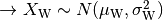
The test suite buildings-shadowing-test is a unit test intended to verify the statistical distribution of the shadowing model implemented by BuildingsPathlossModel. The shadowing is modeled according to a normal distribution with mean  and variable standard deviation
  , according to models commonly used in literature. Three test cases are provided, which cover the cases of indoor, outdoor and indoor-to-outdoor communications.
Each test case generates 1000 different samples of shadowing for different pairs of MobilityModel instances in a given scenario. Shadowing values are obtained by subtracting from the total loss value returned by
, according to models commonly used in literature. Three test cases are provided, which cover the cases of indoor, outdoor and indoor-to-outdoor communications.
Each test case generates 1000 different samples of shadowing for different pairs of MobilityModel instances in a given scenario. Shadowing values are obtained by subtracting from the total loss value returned by HybridBuildingsPathlossModel the path loss component which is constant and pre-determined for each test case. The test verifies that the sample mean and sample variance of the shadowing values fall within the 99% confidence interval of the sample mean and sample variance. The test also verifies that the shadowing values returned at successive times for the same pair of MobilityModel instances is constant.
Buildings Channel Condition Model Test
The BuildingsChannelConditionModelTestSuite tests the class BuildingsChannelConditionModel. It checks if the channel condition between two nodes is correctly determined when a building is deployed.
References
| [turkmani] | Turkmani A.M.D., J.D. Parson and D.G. Lewis, “Radio propagation into buildings at 441, 900 and 1400 MHz”, in Proc. of 4th Int. Conference on Land Mobile Radio, 1987. |
Click Modular Router Integration
Click is a software architecture for building configurable routers. By using different combinations of packet processing units called elements, a Click router can be made to perform a specific kind of functionality. This flexibility provides a good platform for testing and experimenting with different protocols.
Model Description
The source code for the Click model lives in the directory src/click.
Design
ns-3’s design is well suited for an integration with Click due to the following reasons:
- Packets in ns-3 are serialised/deserialised as they move up/down the stack. This allows ns-3 packets to be passed to and from Click as they are.
- This also means that any kind of ns-3 traffic generator and transport should work easily on top of Click.
- By striving to implement click as an Ipv4RoutingProtocol instance, we can avoid significant changes to the LL and MAC layer of the ns-3 code.
The design goal was to make the ns-3-click public API simple enough such that the user needs to merely add an Ipv4ClickRouting instance to the node, and inform each Click node of the Click configuration file (.click file) that it is to use.
This model implements the interface to the Click Modular Router and provides the Ipv4ClickRouting class to allow a node to use Click for external routing. Unlike normal Ipv4RoutingProtocol sub types, Ipv4ClickRouting doesn’t use a RouteInput() method, but instead, receives a packet on the appropriate interface and processes it accordingly. Note that you need to have a routing table type element in your Click graph to use Click for external routing. This is needed by the RouteOutput() function inherited from Ipv4RoutingProtocol. Furthermore, a Click based node uses a different kind of L3 in the form of Ipv4L3ClickProtocol, which is a trimmed down version of Ipv4L3Protocol. Ipv4L3ClickProtocol passes on packets passing through the stack to Ipv4ClickRouting for processing.
Developing a Simulator API to allow ns-3 to interact with Click
Much of the API is already well defined, which allows Click to probe for information from the simulator (like a Node’s ID, an Interface ID and so forth). By retaining most of the methods, it should be possible to write new implementations specific to ns-3 for the same functionality.
Hence, for the Click integration with ns-3, a class named Ipv4ClickRouting will handle the interaction with Click. The code for the same can be found in src/click/model/ipv4-click-routing.{cc,h}.
Packet hand off between ns-3 and Click
There are four kinds of packet hand-offs that can occur between ns-3 and Click.
- L4 to L3
- L3 to L4
- L3 to L2
- L2 to L3
To overcome this, we implement Ipv4L3ClickProtocol, a stripped down version of Ipv4L3Protocol. Ipv4L3ClickProtocol passes packets to and from Ipv4ClickRouting appropriately to perform routing.
Scope and Limitations
- In its current state, the NS-3 Click Integration is limited to use only with L3, leaving NS-3 to handle L2. We are currently working on adding Click MAC support as well. See the usage section to make sure that you design your Click graphs accordingly.
- Furthermore, ns-3-click will work only with userlevel elements. The complete list of elements are available at http://read.cs.ucla.edu/click/elements. Elements that have ‘all’, ‘userlevel’ or ‘ns’ mentioned beside them may be used.
- As of now, the ns-3 interface to Click is Ipv4 only. We will be adding Ipv6 support in the future.
References
- Eddie Kohler, Robert Morris, Benjie Chen, John Jannotti, and M. Frans Kaashoek. The click modular router. ACM Transactions on Computer Systems 18(3), August 2000, pages 263-297.
- Lalith Suresh P., and Ruben Merz. Ns-3-click: click modular router integration for ns-3. In Proc. of 3rd International ICST Workshop on NS-3 (WNS3), Barcelona, Spain. March, 2011.
- Michael Neufeld, Ashish Jain, and Dirk Grunwald. Nsclick: bridging network simulation and deployment. MSWiM ‘02: Proceedings of the 5th ACM international workshop on Modeling analysis and simulation of wireless and mobile systems, 2002, Atlanta, Georgia, USA. http://doi.acm.org/10.1145/570758.570772
Usage
Building Click
The first step is to clone Click from the github repository and build it:
$ git clone https://github.com/kohler/click
$ cd click/
$ ./configure --disable-linuxmodule --enable-nsclick --enable-wifi
$ make
The –enable-wifi flag may be skipped if you don’t intend on using Click with Wifi. * Note: You don’t need to do a ‘make install’.
Once Click has been built successfully, change into the ns-3 directory and configure ns-3 with Click Integration support:
$ ./waf configure --enable-examples --enable-tests --with-nsclick=/path/to/click/source
Hint: If you have click installed one directory above ns-3 (such as in the ns-3-allinone directory), and the name of the directory is ‘click’ (or a symbolic link to the directory is named ‘click’), then the –with-nsclick specifier is not necessary; the ns-3 build system will successfully find the directory.
If it says ‘enabled’ beside ‘NS-3 Click Integration Support’, then you’re good to go. Note: If running modular ns-3, the minimum set of modules required to run all ns-3-click examples is wifi, csma and config-store.
Next, try running one of the examples:
$ ./waf --run nsclick-simple-lan
You may then view the resulting .pcap traces, which are named nsclick-simple-lan-0-0.pcap and nsclick-simple-lan-0-1.pcap.
Click Graph Instructions
The following should be kept in mind when making your Click graph:
- Only userlevel elements can be used.
- You will need to replace FromDevice and ToDevice elements with FromSimDevice and ToSimDevice elements.
- Packets to the kernel are sent up using ToSimDevice(tap0,IP).
- For any node, the device which sends/receives packets to/from the kernel, is named ‘tap0’. The remaining interfaces should be named eth0, eth1 and so forth (even if you’re using wifi). Please note that the device numbering should begin from 0. In future, this will be made flexible so that users can name devices in their Click file as they wish.
- A routing table element is a mandatory. The OUTports of the routing table element should correspond to the interface number of the device through which the packet will ultimately be sent out. Violating this rule will lead to really weird packet traces. This routing table element’s name should then be passed to the Ipv4ClickRouting protocol object as a simulation parameter. See the Click examples for details.
- The current implementation leaves Click with mainly L3 functionality, with ns-3 handling L2. We will soon begin working to support the use of MAC protocols on Click as well. This means that as of now, Click’s Wifi specific elements cannot be used with ns-3.
Debugging Packet Flows from Click
From any point within a Click graph, you may use the Print (http://read.cs.ucla.edu/click/elements/print) element and its variants for pretty printing of packet contents. Furthermore, you may generate pcap traces of packets flowing through a Click graph by using the ToDump (http://read.cs.ucla.edu/click/elements/todump) element as well. For instance:
myarpquerier
 -> Print(fromarpquery,64)
 -> ToDump(out_arpquery,PER_NODE 1)
 -> ethout;
and …will print the contents of packets that flow out of the ArpQuerier, then generate a pcap trace file which will have a suffix ‘out_arpquery’, for each node using the Click file, before pushing packets onto ‘ethout’.
Helper
To have a node run Click, the easiest way would be to use the ClickInternetStackHelper class in your simulation script. For instance:
ClickInternetStackHelper click;
click.SetClickFile (myNodeContainer, "nsclick-simple-lan.click");
click.SetRoutingTableElement (myNodeContainer, "u/rt");
click.Install (myNodeContainer);
The example scripts inside src/click/examples/ demonstrate the use of Click based nodes
in different scenarios. The helper source can be found inside src/click/helper/click-internet-stack-helper.{h,cc}
Examples
The following examples have been written, which can be found in src/click/examples/:
- nsclick-simple-lan.cc and nsclick-raw-wlan.cc: A Click based node communicating with a normal ns-3 node without Click, using Csma and Wifi respectively. It also demonstrates the use of TCP on top of Click, something which the original nsclick implementation for NS-2 couldn’t achieve.
- nsclick-udp-client-server-csma.cc and nsclick-udp-client-server-wifi.cc: A 3 node LAN (Csma and Wifi respectively) wherein 2 Click based nodes run a UDP client, that sends packets to a third Click based node running a UDP server.
- nsclick-routing.cc: One Click based node communicates to another via a third node that acts as an IP router (using the IP router Click configuration). This demonstrates routing using Click.
Scripts are available within <click-dir>/conf/ that allow you to generate Click files for some common scenarios. The IP Router used in nsclick-routing.cc was generated from the make-ip-conf.pl file and slightly adapted to work with ns-3-click.
Validation
This model has been tested as follows:
- Unit tests have been written to verify the internals of Ipv4ClickRouting. This can be found in
src/click/ipv4-click-routing-test.cc. These tests verify whether the methods inside Ipv4ClickRouting which deal with Device name to ID, IP Address from device name and Mac Address from device name bindings work as expected. - The examples have been used to test Click with actual simulation scenarios. These can be found in
src/click/examples/. These tests cover the following: the use of different kinds of transports on top of Click, TCP/UDP, whether Click nodes can communicate with non-Click based nodes, whether Click nodes can communicate with each other, using Click to route packets using static routing. - Click has been tested with Csma, Wifi and Point-to-Point devices. Usage instructions are available in the preceding section.
CSMA NetDevice
This is the introduction to CSMA NetDevice chapter, to complement the CSMA model doxygen.
Overview of the CSMA model
The ns-3 CSMA device models a simple bus network in the spirit of Ethernet. Although it does not model any real physical network you could ever build or buy, it does provide some very useful functionality.
Typically when one thinks of a bus network Ethernet or IEEE 802.3 comes to mind. Ethernet uses CSMA/CD (Carrier Sense Multiple Access with Collision Detection with exponentially increasing backoff to contend for the shared transmission medium. The ns-3 CSMA device models only a portion of this process, using the nature of the globally available channel to provide instantaneous (faster than light) carrier sense and priority-based collision “avoidance.” Collisions in the sense of Ethernet never happen and so the ns-3 CSMA device does not model collision detection, nor will any transmission in progress be “jammed.”
CSMA Layer Model
There are a number of conventions in use for describing layered communications architectures in the literature and in textbooks. The most common layering model is the ISO seven layer reference model. In this view the CsmaNetDevice and CsmaChannel pair occupies the lowest two layers – at the physical (layer one), and data link (layer two) positions. Another important reference model is that specified by RFC 1122, “Requirements for Internet Hosts – Communication Layers.” In this view the CsmaNetDevice and CsmaChannel pair occupies the lowest layer – the link layer. There is also a seemingly endless litany of alternative descriptions found in textbooks and in the literature. We adopt the naming conventions used in the IEEE 802 standards which speak of LLC, MAC, MII and PHY layering. These acronyms are defined as:
- LLC: Logical Link Control;
- MAC: Media Access Control;
- MII: Media Independent Interface;
- PHY: Physical Layer.
In this case the LLC and MAC are sublayers of the OSI data link layer and the MII and PHY are sublayers of the OSI physical layer.
The “top” of the CSMA device defines the transition from the network layer to the data link layer. This transition is performed by higher layers by calling either CsmaNetDevice::Send or CsmaNetDevice::SendFrom.
In contrast to the IEEE 802.3 standards, there is no precisely specified PHY in the CSMA model in the sense of wire types, signals or pinouts. The “bottom” interface of the CsmaNetDevice can be thought of as as a kind of Media Independent Interface (MII) as seen in the “Fast Ethernet” (IEEE 802.3u) specifications. This MII interface fits into a corresponding media independent interface on the CsmaChannel. You will not find the equivalent of a 10BASE-T or a 1000BASE-LX PHY.
The CsmaNetDevice calls the CsmaChannel through a media independent interface. There is a method defined to tell the channel when to start “wiggling the wires” using the method CsmaChannel::TransmitStart, and a method to tell the channel when the transmission process is done and the channel should begin propagating the last bit across the “wire”: CsmaChannel::TransmitEnd.
When the TransmitEnd method is executed, the channel will model a single uniform signal propagation delay in the medium and deliver copes of the packet to each of the devices attached to the packet via the CsmaNetDevice::Receive method.
There is a “pin” in the device media independent interface corresponding to “COL” (collision). The state of the channel may be sensed by calling CsmaChannel::GetState. Each device will look at this “pin” before starting a send and will perform appropriate backoff operations if required.
Properly received packets are forwarded up to higher levels from the CsmaNetDevice via a callback mechanism. The callback function is initialized by the higher layer (when the net device is attached) using CsmaNetDevice::SetReceiveCallback and is invoked upon “proper” reception of a packet by the net device in order to forward the packet up the protocol stack.
CSMA Channel Model
The class CsmaChannel models the actual transmission medium. There is no fixed limit for the number of devices connected to the channel. The CsmaChannel models a data rate and a speed-of-light delay which can be accessed via the attributes “DataRate” and “Delay” respectively. The data rate provided to the channel is used to set the data rates used by the transmitter sections of the CSMA devices connected to the channel. There is no way to independently set data rates in the devices. Since the data rate is only used to calculate a delay time, there is no limitation (other than by the data type holding the value) on the speed at which CSMA channels and devices can operate; and no restriction based on any kind of PHY characteristics.
The CsmaChannel has three states, IDLE, TRANSMITTING and
PROPAGATING. These three states are “seen” instantaneously by all devices on
the channel. By this we mean that if one device begins or ends a simulated
transmission, all devices on the channel are immediately aware of the
change in state. There is no time during which one device may see an IDLE
channel while another device physically further away in the collision domain may
have begun transmitting with the associated signals not propagated down the
channel to other devices. Thus there is no need for collision detection in the
CsmaChannel model and it is not implemented in any way.
We do, as the name indicates, have a Carrier Sense aspect to the model. Since
the simulator is single threaded, access to the common channel will be
serialized by the simulator. This provides a deterministic mechanism for
contending for the channel. The channel is allocated (transitioned from state
IDLE to state TRANSMITTING) on a first-come first-served basis.
The channel always goes through a three state process:
IDLE -> TRANSMITTING -> PROPAGATING -> IDLE
The TRANSMITTING state models the time during which the source net device is
actually wiggling the signals on the wire. The PROPAGATING state models the
time after the last bit was sent, when the signal is propagating down the wire
to the “far end.”
The transition to the TRANSMITTING state is driven by a call to
CsmaChannel::TransmitStart which is called by the net device that transmits the
packet. It is the responsibility of that device to end the transmission with a
call to CsmaChannel::TransmitEnd at the appropriate simulation time that
reflects the time elapsed to put all of the packet bits on the wire. When
TransmitEnd is called, the channel schedules an event corresponding to a single
speed-of-light delay. This delay applies to all net devices on the channel
identically. You can think of a symmetrical hub in which the packet bits
propagate to a central location and then back out equal length cables to the
other devices on the channel. The single “speed of light” delay then corresponds
to the time it takes for: 1) a signal to propagate from one CsmaNetDevice
through its cable to the hub; plus 2) the time it takes for the hub to forward
the packet out a port; plus 3) the time it takes for the signal in question to
propagate to the destination net device.
The CsmaChannel models a broadcast medium so the packet is delivered to all of the devices on the channel (including the source) at the end of the propagation time. It is the responsibility of the sending device to determine whether or not it receives a packet broadcast over the channel.
The CsmaChannel provides following Attributes:
- DataRate: The bitrate for packet transmission on connected devices;
- Delay: The speed of light transmission delay for the channel.
CSMA Net Device Model
The CSMA network device appears somewhat like an Ethernet device. The CsmaNetDevice provides following Attributes:
- Address: The Mac48Address of the device;
- SendEnable: Enable packet transmission if true;
- ReceiveEnable: Enable packet reception if true;
- EncapsulationMode: Type of link layer encapsulation to use;
- RxErrorModel: The receive error model;
- TxQueue: The transmit queue used by the device;
- InterframeGap: The optional time to wait between “frames”;
- Rx: A trace source for received packets;
- Drop: A trace source for dropped packets.
The CsmaNetDevice supports the assignment of a “receive error model.” This is an ErrorModel object that is used to simulate data corruption on the link.
Packets sent over the CsmaNetDevice are always routed through the transmit queue to provide a trace hook for packets sent out over the network. This transmit queue can be set (via attribute) to model different queuing strategies.
Also configurable by attribute is the encapsulation method used by the device. Every packet gets an EthernetHeader that includes the destination and source MAC addresses, and a length/type field. Every packet also gets an EthernetTrailer which includes the FCS. Data in the packet may be encapsulated in different ways.
By default, or by setting the “EncapsulationMode” attribute to “Dix”, the encapsulation is according to the DEC, Intel, Xerox standard. This is sometimes called EthernetII framing and is the familiar destination MAC, source MAC, EtherType, Data, CRC format.
If the “EncapsulationMode” attribute is set to “Llc”, the encapsulation is by LLC SNAP. In this case, a SNAP header is added that contains the EtherType (IP or ARP).
The other implemented encapsulation modes are IP_ARP (set “EncapsulationMode” to “IpArp”) in which the length type of the Ethernet header receives the protocol number of the packet; or ETHERNET_V1 (set “EncapsulationMode” to “EthernetV1”) in which the length type of the Ethernet header receives the length of the packet. A “Raw” encapsulation mode is defined but not implemented – use of the RAW mode results in an assertion.
Note that all net devices on a channel must be set to the same encapsulation mode for correct results. The encapsulation mode is not sensed at the receiver.
The CsmaNetDevice implements a random exponential backoff algorithm that is
executed if the channel is determined to be busy (TRANSMITTING or
PPROPAGATING) when the device wants to start propagating. This results in a
random delay of up to pow (2, retries) - 1 microseconds before a retry is
attempted. The default maximum number of retries is 1000.
Using the CsmaNetDevice
The CSMA net devices and channels are typically created and configured using the
associated CsmaHelper object. The various ns-3 device helpers generally
work in a similar way, and their use is seen in many of our example programs.
The conceptual model of interest is that of a bare computer “husk” into which
you plug net devices. The bare computers are created using a NodeContainer
helper. You just ask this helper to create as many computers (we call them
Nodes) as you need on your network:
NodeContainer csmaNodes;
csmaNodes.Create (nCsmaNodes);
Once you have your nodes, you need to instantiate a CsmaHelper and set any
attributes you may want to change.:
CsmaHelper csma;
csma.SetChannelAttribute ("DataRate", StringValue ("100Mbps"));
csma.SetChannelAttribute ("Delay", TimeValue (NanoSeconds (6560)));

csma.SetDeviceAttribute ("EncapsulationMode", StringValue ("Dix"));
csma.SetDeviceAttribute ("FrameSize", UintegerValue (2000));
Once the attributes are set, all that remains is to create the devices and install them on the required nodes, and to connect the devices together using a CSMA channel. When we create the net devices, we add them to a container to allow you to use them in the future. This all takes just one line of code.:
NetDeviceContainer csmaDevices = csma.Install (csmaNodes);
We recommend thinking carefully about changing these Attributes, since it can result in behavior that surprises users. We allow this because we believe flexibility is important. As an example of a possibly surprising effect of changing Attributes, consider the following:
The Mtu Attribute indicates the Maximum Transmission Unit to the device. This is the size of the largest Protocol Data Unit (PDU) that the device can send. This Attribute defaults to 1500 bytes and corresponds to a number found in RFC 894, “A Standard for the Transmission of IP Datagrams over Ethernet Networks.” The number is actually derived from the maximum packet size for 10Base5 (full-spec Ethernet) networks – 1518 bytes. If you subtract DIX encapsulation overhead for Ethernet packets (18 bytes) you will end up with a maximum possible data size (MTU) of 1500 bytes. One can also find that the MTU for IEEE 802.3 networks is 1492 bytes. This is because LLC/SNAP encapsulation adds an extra eight bytes of overhead to the packet. In both cases, the underlying network hardware is limited to 1518 bytes, but the MTU is different because the encapsulation is different.
If one leaves the Mtu Attribute at 1500 bytes and changes the encapsulation mode Attribute to Llc, the result will be a network that encapsulates 1500 byte PDUs with LLC/SNAP framing resulting in packets of 1526 bytes. This would be illegal in many networks, but we allow you do do this. This results in a simulation that quite subtly does not reflect what you might be expecting since a real device would balk at sending a 1526 byte packet.
There also exist jumbo frames (1500 < MTU <= 9000 bytes) and super-jumbo (MTU > 9000 bytes) frames that are not officially sanctioned by IEEE but are available in some high-speed (Gigabit) networks and NICs. In the CSMA model, one could leave the encapsulation mode set to Dix, and set the Mtu to 64000 bytes – even though an associated CsmaChannel DataRate was left at 10 megabits per second (certainly not Gigabit Ethernet). This would essentially model an Ethernet switch made out of vampire-tapped 1980s-style 10Base5 networks that support super-jumbo datagrams, which is certainly not something that was ever made, nor is likely to ever be made; however it is quite easy for you to configure.
Be careful about assumptions regarding what CSMA is actually modelling and how configuration (Attributes) may allow you to swerve considerably away from reality.
CSMA Tracing
Like all ns-3 devices, the CSMA Model provides a number of trace sources. These trace sources can be hooked using your own custom trace code, or you can use our helper functions to arrange for tracing to be enabled on devices you specify.
Upper-Level (MAC) Hooks
From the point of view of tracing in the net device, there are several interesting points to insert trace hooks. A convention inherited from other simulators is that packets destined for transmission onto attached networks pass through a single “transmit queue” in the net device. We provide trace hooks at this point in packet flow, which corresponds (abstractly) only to a transition from the network to data link layer, and call them collectively the device MAC hooks.
When a packet is sent to the CSMA net device for transmission it always passes through the transmit queue. The transmit queue in the CsmaNetDevice inherits from Queue, and therefore inherits three trace sources:
- An Enqueue operation source (see Queue::m_traceEnqueue);
- A Dequeue operation source (see Queue::m_traceDequeue);
- A Drop operation source (see Queue::m_traceDrop).
The upper-level (MAC) trace hooks for the CsmaNetDevice are, in fact, exactly these three trace sources on the single transmit queue of the device.
The m_traceEnqueue event is triggered when a packet is placed on the transmit queue. This happens at the time that CsmaNetDevice::Send or CsmaNetDevice::SendFrom is called by a higher layer to queue a packet for transmission.
The m_traceDequeue event is triggered when a packet is removed from the transmit queue. Dequeues from the transmit queue can happen in three situations: 1) If the underlying channel is idle when the CsmaNetDevice::Send or CsmaNetDevice::SendFrom is called, a packet is dequeued from the transmit queue and immediately transmitted; 2) If the underlying channel is idle, a packet may be dequeued and immediately transmitted in an internal TransmitCompleteEvent that functions much like a transmit complete interrupt service routine; or 3) from the random exponential backoff handler if a timeout is detected.
Case (3) implies that a packet is dequeued from the transmit queue if it is unable to be transmitted according to the backoff rules. It is important to understand that this will appear as a Dequeued packet and it is easy to incorrectly assume that the packet was transmitted since it passed through the transmit queue. In fact, a packet is actually dropped by the net device in this case. The reason for this behavior is due to the definition of the Queue Drop event. The m_traceDrop event is, by definition, fired when a packet cannot be enqueued on the transmit queue because it is full. This event only fires if the queue is full and we do not overload this event to indicate that the CsmaChannel is “full.”
Lower-Level (PHY) Hooks
Similar to the upper level trace hooks, there are trace hooks available at the lower levels of the net device. We call these the PHY hooks. These events fire from the device methods that talk directly to the CsmaChannel.
The trace source m_dropTrace is called to indicate a packet that is dropped by the device. This happens in two cases: First, if the receive side of the net device is not enabled (see CsmaNetDevice::m_receiveEnable and the associated attribute “ReceiveEnable”).
The m_dropTrace is also used to indicate that a packet was discarded as corrupt if a receive error model is used (see CsmaNetDevice::m_receiveErrorModel and the associated attribute “ReceiveErrorModel”).
The other low-level trace source fires on reception of an accepted packet (see CsmaNetDevice::m_rxTrace). A packet is accepted if it is destined for the broadcast address, a multicast address, or to the MAC address assigned to the net device.
Summary
The ns3 CSMA model is a simplistic model of an Ethernet-like network. It supports a Carrier-Sense function and allows for Multiple Access to a shared medium. It is not physical in the sense that the state of the medium is instantaneously shared among all devices. This means that there is no collision detection required in this model and none is implemented. There will never be a “jam” of a packet already on the medium. Access to the shared channel is on a first-come first-served basis as determined by the simulator scheduler. If the channel is determined to be busy by looking at the global state, a random exponential backoff is performed and a retry is attempted.
Ns-3 Attributes provide a mechanism for setting various parameters in the device and channel such as addresses, encapsulation modes and error model selection. Trace hooks are provided in the usual manner with a set of upper level hooks corresponding to a transmit queue and used in ASCII tracing; and also a set of lower level hooks used in pcap tracing.
Although the ns-3 CsmaChannel and CsmaNetDevice does not model any kind of network you could build or buy, it does provide us with some useful functionality. You should, however, understand that it is explicitly not Ethernet or any flavor of IEEE 802.3 but an interesting subset.
DSDV Routing
Destination-Sequenced Distance Vector (DSDV) routing protocol is a pro-active, table-driven routing protocol for MANETs developed by Charles E. Perkins and Pravin Bhagwat in 1994. It uses the hop count as metric in route selection.
This model was developed by the ResiliNets research group at the University of Kansas. A paper on this model exists at this URL.
DSDV Routing Overview
DSDV Routing Table: Every node will maintain a table listing all the other nodes it has known either directly or through some neighbors. Every node has a single entry in the routing table. The entry will have information about the node’s IP address, last known sequence number and the hop count to reach that node. Along with these details the table also keeps track of the nexthop neighbor to reach the destination node, the timestamp of the last update received for that node.
The DSDV update message consists of three fields, Destination Address, Sequence Number and Hop Count.
Each node uses 2 mechanisms to send out the DSDV updates. They are,
- Periodic Updates
- Periodic updates are sent out after every m_periodicUpdateInterval(default:15s). In this update the node broadcasts out its entire routing table.
- Trigger Updates
- Trigger Updates are small updates in-between the periodic updates. These updates are sent out whenever a node receives a DSDV packet that caused a change in its routing table. The original paper did not clearly mention when for what change in the table should a DSDV update be sent out. The current implementation sends out an update irrespective of the change in the routing table.
The updates are accepted based on the metric for a particular node. The first factor determining the acceptance of an update is the sequence number. It has to accept the update if the sequence number of the update message is higher irrespective of the metric. If the update with same sequence number is received, then the update with least metric (hopCount) is given precedence.
In highly mobile scenarios, there is a high chance of route fluctuations, thus we have the concept of weighted settling time where an update with change in metric will not be advertised to neighbors. The node waits for the settling time to make sure that it did not receive the update from its old neighbor before sending out that update.
The current implementation covers all the above features of DSDV. The current implementation also has a request queue to buffer packets that have no routes to destination. The default is set to buffer up to 5 packets per destination.
References
Link to the Paper: http://portal.acm.org/citation.cfm?doid=190314.190336
DSR Routing
Dynamic Source Routing (DSR) protocol is a reactive routing protocol designed specifically for use in multi-hop wireless ad hoc networks of mobile nodes.
This model was developed by the ResiliNets research group at the University of Kansas.
DSR Routing Overview
This model implements the base specification of the Dynamic Source Routing (DSR) protocol. Implementation is based on RFC 4728, with some extensions and modifications to the RFC specifications.
DSR operates on a on-demand behavior. Therefore, our DSR model buffers all packets while a route request packet (RREQ) is disseminated. We implement a packet buffer in dsr-rsendbuff.cc. The packet queue implements garbage collection of old packets and a queue size limit. When the packet is sent out from the send buffer, it will be queued in maintenance buffer for next hop acknowledgment.
The maintenance buffer then buffers the already sent out packets and waits for the notification of packet delivery. Protocol operation strongly depends on broken link detection mechanism. We implement the three heuristics recommended based the RFC as follows:
First, we use link layer feedback when possible, which is also the fastest mechanism of these three to detect link errors. A link is considered to be broken if frame transmission results in a transmission failure for all retries. This mechanism is meant for active links and works much faster than in its absence. DSR is able to detect the link layer transmission failure and notify that as broken. Recalculation of routes will be triggered when needed. If user does not want to use link layer acknowledgment, it can be tuned by setting “LinkAcknowledgment” attribute to false in “dsr-routing.cc”.
Second, passive acknowledgment should be used whenever possible. The node turns on “promiscuous” receive mode, in which it can receive packets not destined for itself, and when the node assures the delivery of that data packet to its destination, it cancels the passive acknowledgment timer.
Last, we use a network layer acknowledge scheme to notify the receipt of a packet. Route request packet will not be acknowledged or retransmitted.
The Route Cache implementation support garbage collection of old entries and state machine, as defined in the standard. It implements as a STL map container. The key is the destination IP address.
DSR operates with direct access to IP header, and operates between network and transport layer. When packet is sent out from transport layer, it passes itself to DSR and DSR header is appended.
We have two caching mechanisms: path cache and link cache. The path cache saves the whole path in the cache. The paths are sorted based on the hop count, and whenever one path is not able to be used, we change to the next path. The link cache is a slightly better design in the sense that it uses different subpaths and uses Implemented Link Cache using Dijkstra algorithm, and this part is implemented by Song Luan <lsuper@mail.ustc.edu.cn>.
The following optional protocol optimizations aren’t implemented:
- Flow state
- First Hop External (F), Last Hop External (L) flags
- Handling unknown DSR options
- Two types of error headers:
- flow state not supported option
- unsupported option (not going to happen in simulation)
DSR update in ns-3.17
We originally used “TxErrHeader” in Ptr<WifiMac> to indicate the transmission error of a specific packet in link layer, however, it was not working quite correctly since even when the packet was dropped, this header was not recorded in the trace file. We used to a different path on implementing the link layer notification mechanism. We look into the trace file by finding packet receive event. If we find one receive event for the data packet, we count that as the indicator for successful data delivery.
Useful parameters
+------------------------- +------------------------------------+-------------+
| Parameter                | Description                        | Default     |
+==========================+====================================+=============+
| MaxSendBuffLen           | Maximum number of packets that can | 64          |
|                          | be stored in send buffer           |             |
+------------------------- +------------------------------------+-------------+
| MaxSendBuffTime          | Maximum time packets can be queued | Seconds(30) |
|                          | in the send buffer                 |             |
+------------------------- +------------------------------------+-------------+
| MaxMaintLen              | Maximum number of packets that can | 50          |
|                          | be stored in maintenance buffer    |             |
+------------------------- +------------------------------------+-------------+
| MaxMaintTime             | Maximum time packets can be queued | Seconds(30) |
|                          | in maintenance buffer              |             |
+------------------------- +------------------------------------+-------------+
| MaxCacheLen              | Maximum number of route entries    | 64          |
|                          | that can be stored in route cache  |             |
+------------------------- +------------------------------------+-------------+
| RouteCacheTimeout        | Maximum time the route cache can   | Seconds(300)|
|                          | be queued in route cache           |             |
+------------------------- +------------------------------------+-------------+
| RreqRetries              | Maximum number of retransmissions  | 16          |
|                          | for request discovery of a route   |             |
+------------------------- +------------------------------------+-------------+
| CacheType                | Use Link Cache or use Path Cache   | "LinkCache" |
|                          |                                    |             |
+------------------------- +------------------------------------+-------------+
| LinkAcknowledgment       | Enable Link layer acknowledgment   | True        |
|                          | mechanism                          |             |
+------------------------- +------------------------------------+-------------+
Implementation modification
- The DsrFsHeader has added 3 fields: message type, source id, destination id, and these changes only for post-processing
- Message type is used to identify the data packet from control packet
- source id is used to identify the real source of the data packet since we have to deliver the packet hop-by-hop and the Ipv4Header is not carrying the real source and destination ip address as needed
- destination id is for same reason of above
- Route Reply header is not word-aligned in DSR RFC, change it to word-aligned in implementation
- DSR works as a shim header between transport and network protocol, it needs its own forwarding mechanism, we are changing the packet transmission to hop-by-hop delivery, so we added two fields in dsr fixed header to notify packet delivery
Current Route Cache implementation
This implementation used “path cache”, which is simple to implement and ensures loop-free paths:
- the path cache has automatic expire policy
- the cache saves multiple route entries for a certain destination and sort the entries based on hop counts
- the MaxEntriesEachDst can be tuned to change the maximum entries saved for a single destination
- when adding multiple routes for one destination, the route is compared based on hop-count and expire time, the one with less hop count or relatively new route is favored
- Future implementation may include “link cache” as another possibility
DSR Instructions
The following should be kept in mind when running DSR as routing protocol:
- NodeTraversalTime is the time it takes to traverse two neighboring nodes and should be chosen to fit the transmission range
- PassiveAckTimeout is the time a packet in maintenance buffer wait for passive acknowledgment, normally set as two times of NodeTraversalTime
- RouteCacheTimeout should be set smaller value when the nodes’ velocity become higher. The default value is 300s.
Helper
To have a node run DSR, the easiest way would be to use the DsrHelper and DsrMainHelpers in your simulation script. For instance:
DsrHelper dsr;
DsrMainHelper dsrMain;
dsrMain.Install (dsr, adhocNodes);
The example scripts inside src/dsr/examples/ demonstrate the use of DSR based nodes in different scenarios.
The helper source can be found inside src/dsr/helper/dsr-main-helper.{h,cc}
and src/dsr/helper/dsr-helper.{h,cc}
Examples
The example can be found in src/dsr/examples/:
- dsr.cc use DSR as routing protocol within a traditional MANETs environment[3].
DSR is also built in the routing comparison case in examples/routing/:
manet-routing-compare.ccis a comparison case with built in MANET routing protocols and can generate its own results.
Validation
This model has been tested as follows:
- Unit tests have been written to verify the internals of DSR. This can be found in
src/dsr/test/dsr-test-suite.cc. These tests verify whether the methods inside DSR module which deal with packet buffer, headers work correctly. - Simulation cases similar to [3] have been tested and have comparable results.
- manet-routing-compare.cc has been used to compare DSR with three of other routing protocols.
A paper was presented on these results at the Workshop on ns-3 in 2011.
Limitations
The model is not fully compliant with RFC 4728. As an example, Dsr fixed size header has been extended and it is four octets longer then the RFC specification. As a consequence, the DSR headers can not be correctly decoded by Wireshark.
The model full compliance with the RFC is planned for the future.
References
[1] Original paper: http://www.monarch.cs.rice.edu/monarch-papers/dsr-chapter00.pdf
[2] RFC 4728 http://www6.ietf.org/rfc/rfc4728.txt
[3] Broch’s comparison paper: http://www.monarch.cs.rice.edu/monarch-papers/mobicom98.ps
Emulation Overview
ns-3 has been designed for integration into testbed and virtual machine
environments. We have addressed this need by providing two kinds of net devices.
The first kind of device is a file descriptor net device (FdNetDevice),
which is a generic device type that can read and write from a file descriptor.
By associating this file descriptor with different things on the host
system, different capabilities can be provided. For instance, the
FdNetDevice can be associated with an underlying packet socket to provide
emulation capabilities. This allows ns-3 simulations
to send data on a “real” network. The second kind, called a TapBridge
NetDevice allows a “real” host to participate in an ns-3 simulation as if
it were one of the simulated nodes. An ns-3 simulation may be constructed with
any combination of simulated or emulated devices.
Note: Prior to ns-3.17, the emulation capability was provided by a
special device called an Emu NetDevice; the Emu NetDevice has
been replaced by the FdNetDevice.
One of the use-cases we want to support is that of a testbed. A concrete example
of an environment of this kind is the ORBIT testbed. ORBIT is a laboratory
emulator/field trial network arranged as a two dimensional grid of 400 802.11
radio nodes. We integrate with ORBIT by using their “imaging” process to load
and run ns-3 simulations on the ORBIT array. We can use our
EmuFdNetDevice
to drive the hardware in the testbed and we can accumulate results either using
the ns-3 tracing and logging functions, or the native ORBIT data gathering
techniques. See http://www.orbit-lab.org/ for details on the ORBIT
testbed.
A simulation of this kind is shown in the following figure:
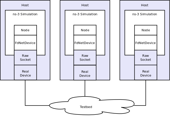
Example Implementation of Testbed Emulation.
You can see that there are separate hosts, each running a subset of a “global” simulation. Instead of an ns-3 channel connecting the hosts, we use real hardware provided by the testbed. This allows ns-3 applications and protocol stacks attached to a simulation node to communicate over real hardware.
We expect the primary use for this configuration will be to generate repeatable experimental results in a real-world network environment that includes all of the ns-3 tracing, logging, visualization and statistics gathering tools.
In what can be viewed as essentially an inverse configuration, we allow “real” machines running native applications and protocol stacks to integrate with an ns-3 simulation. This allows for the simulation of large networks connected to a real machine, and also enables virtualization. A simulation of this kind is shown in the following figure:
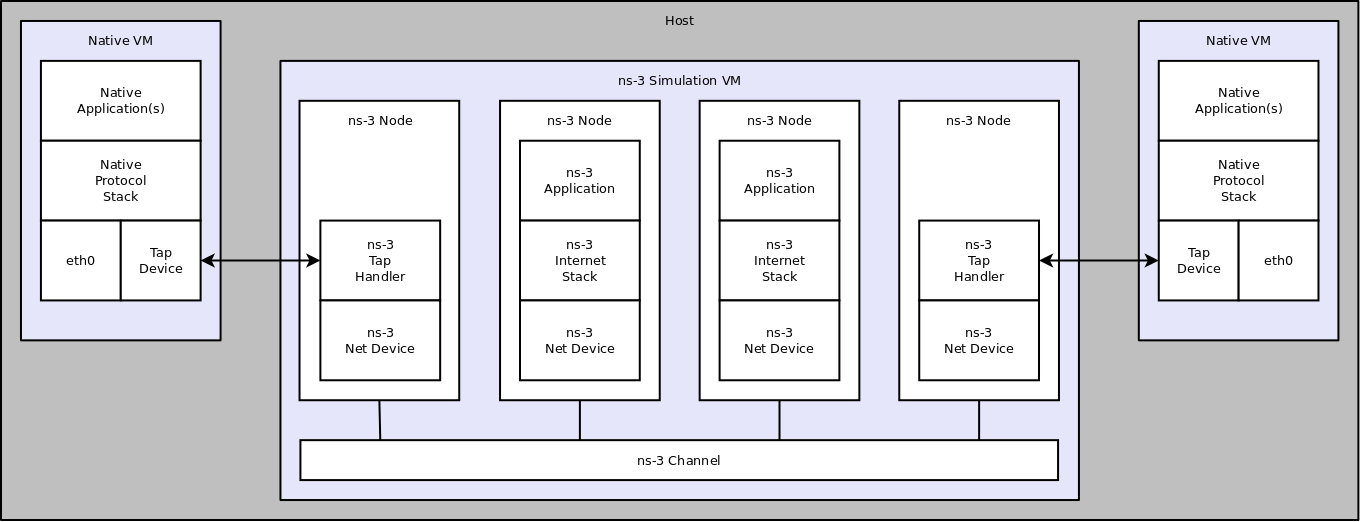
Implementation overview of emulated channel.
Here, you will see that there is a single host with a number of virtual machines running on it. An ns-3 simulation is shown running in the virtual machine shown in the center of the figure. This simulation has a number of nodes with associated ns-3 applications and protocol stacks that are talking to an ns-3 channel through native simulated ns-3 net devices.
There are also two virtual machines shown at the far left and far right of the figure. These VMs are running native (Linux) applications and protocol stacks. The VM is connected into the simulation by a Linux Tap net device. The user-mode handler for the Tap device is instantiated in the simulation and attached to a proxy node that represents the native VM in the simulation. These handlers allow the Tap devices on the native VMs to behave as if they were ns-3 net devices in the simulation VM. This, in turn, allows the native software and protocol suites in the native VMs to believe that they are connected to the simulated ns-3 channel.
We expect the typical use case for this environment will be to analyze the behavior of native applications and protocol suites in the presence of large simulated ns-3 networks.
The basic testbed mode of emulation uses raw sockets. Two other variants (netmap-based and DPDK-based emulation) have been recently added; these make use of more recent network interface cards that make use of directly-mapped memory capabilities to improve packet processing efficiency.
For more details:
File Descriptor NetDevice
The src/fd-net-device module provides the FdNetDevice class,
which is able to read and write traffic using a file descriptor
provided by the user. This file descriptor can be associated to a TAP
device, to a raw socket, to a user space process generating/consuming
traffic, etc.
The user has full freedom to define how external traffic is generated
and ns-3 traffic is consumed.
Different mechanisms to associate a simulation to external traffic can be provided through helper classes. Three specific helpers are provided:
- EmuFdNetDeviceHelper (to associate the ns-3 device with a physical device in the host machine)
- TapFdNetDeviceHelper (to associate the ns-3 device with the file descriptor from a tap device in the host machine)
- PlanteLabFdNetDeviceHelper (to automate the creation of tap devices in PlanetLab nodes, enabling ns-3 simulations that can send and receive traffic though the Internet using PlanetLab resource.
Model Description
The source code for this module lives in the directory src/fd-net-device.
The FdNetDevice is a special type of ns-3 NetDevice that reads traffic to and from a file descriptor. That is, unlike pure simulation NetDevice objects that write frames to and from a simulated channel, this FdNetDevice directs frames out of the simulation to a file descriptor. The file descriptor may be associated to a Linux TUN/TAP device, to a socket, or to a user-space process.
It is up to the user of this device to provide a file descriptor. The type of file descriptor being provided determines what is being modelled. For instance, if the file descriptor provides a raw socket to a WiFi card on the host machine, the device being modelled is a WiFi device.
From the conceptual “top” of the device looking down, it looks to the simulated node like a device supporting a 48-bit IEEE MAC address that can be bridged, supports broadcast, and uses IPv4 ARP or IPv6 Neighbor Discovery, although these attributes can be tuned on a per-use-case basis.
Design
The FdNetDevice implementation makes use of a reader object,
extended from the FdReader class in the ns-3 src/core module,
which manages a separate thread from the main ns-3 execution thread, in order
to read traffic from the file descriptor.
Upon invocation of the StartDevice method, the reader object is initialized
and starts the reading thread.
Before device start, a file descriptor must be previously associated to the
FdNetDevice with the SetFileDescriptor invocation.
The creation and configuration of the file descriptor can be left to a
number of helpers, described in more detail below. When this is done, the
invocation of SetFileDescriptor is responsibility of
the helper and must not be directly invoked by the user.
Upon reading an incoming frame from the file descriptor, the reader
will pass the frame to the ReceiveCallback method, whose
task it is to schedule the reception of the frame by the device as a
ns-3 simulation event. Since the new frame is passed from the reader
thread to the main ns-3 simulation thread, thread-safety issues
are avoided by using the ScheduleWithContext call instead of the
regular Schedule call.
In order to avoid overwhelming the scheduler when the incoming data rate
is too high, a counter is kept with the number of frames that are currently
scheduled to be received by the device. If this counter reaches the value
given by the RxQueueSize attribute in the device, then the new frame will
be dropped silently.
The actual reception of the new frame by the device occurs when the
scheduled FordwarUp method is invoked by the simulator.
This method acts as if a new frame had arrived from a channel attached
to the device. The device then decapsulates the frame, removing any layer 2
headers, and forwards it to upper network stack layers of the node.
The ForwardUp method will remove the frame headers,
according to the frame encapsulation type defined by the EncapsulationMode
attribute, and invoke the receive callback passing an IP packet.
An extra header, the PI header, can be present when the file descriptor is
associated to a TAP device that was created without setting the IFF_NO_PI flag.
This extra header is removed if EncapsulationMode is set to DIXPI value.
In the opposite direction, packets generated inside the simulation that are
sent out through the device, will be passed to the Send method, which
will in turn invoke the SendFrom method. The latter method will add the
necessary layer 2 headers, and simply write the newly created frame to the
file descriptor.
Scope and Limitations
Users of this device are cautioned that there is no flow control across the file descriptor boundary, when using in emulation mode. That is, in a Linux system, if the speed of writing network packets exceeds the ability of the underlying physical device to buffer the packets, backpressure up to the writing application will be applied to avoid local packet loss. No such flow control is provided across the file descriptor interface, so users must be aware of this limitation.
As explained before, the RxQueueSize attribute limits the number of packets that can be pending to be received by the device. Frames read from the file descriptor while the number of pending packets is in its maximum will be silently dropped.
The mtu of the device defaults to the Ethernet II MTU value. However, helpers
are supposed to set the mtu to the right value to reflect the characteristics
of the network interface associated to the file descriptor.
If no helper is used, then the responsibility of setting the correct mtu value
for the device falls back to the user.
The size of the read buffer on the file descriptor reader is set to the
mtu value in the StartDevice method.
The FdNetDevice class currently supports three encapsulation modes, DIX for Ethernet II frames, LLC for 802.2 LLC/SNAP frames, and DIXPI for Ethernet II frames with an additional TAP PI header. This means that traffic traversing the file descriptor is expected to be Ethernet II compatible. IEEE 802.1q (VLAN) tagging is not supported. Attaching an FdNetDevice to a wireless interface is possible as long as the driver provides Ethernet II frames to the socket API. Note that to associate a FdNetDevice to a wireless card in ad-hoc mode, the MAC address of the device must be set to the real card MAC address, else any incoming traffic a fake MAC address will be discarded by the driver.
As mentioned before, three helpers are provided with the fd-net-device module.
Each individual helper (file descriptor type) may have platform
limitations. For instance, threading, real-time simulation mode, and the
ability to create TUN/TAP devices are prerequisites to using the
provided helpers. Support for these modes can be found in the output
of the waf configure step, e.g.:
Threading Primitives          : enabled
Real Time Simulator           : enabled
Emulated Net Device           : enabled
Tap Bridge                    : enabled
It is important to mention that while testing the FdNetDevice we have found
an upper bound limit for TCP throughput when using 1Gb Ethernet links of 60Mbps.
This limit is most likely due to the processing power of the computers involved
in the tests.
Usage
The usage pattern for this type of device is similar to other net devices
with helpers that install to node pointers or node containers.
When using the base FdNetDeviceHelper the user is responsible for
creating and setting the file descriptor by himself.
FdNetDeviceHelper fd;
NetDeviceContainer devices = fd.Install (nodes);

// file descriptor generation
...

device->SetFileDescriptor (fd);
Most commonly a FdNetDevice will be used to interact with the host system. In these cases it is almost certain that the user will want to run in real-time emulation mode, and to enable checksum computations. The typical program statements are as follows:
GlobalValue::Bind ("SimulatorImplementationType", StringValue ("ns3::RealtimeSimulatorImpl"));
GlobalValue::Bind ("ChecksumEnabled", BooleanValue (true));
The easiest way to set up an experiment that interacts with a Linux host
system is to user the Emu and Tap helpers.
Perhaps the most unusual part of these helper implementations
relates to the requirement for executing some of the code with super-user
permissions. Rather than force the user to execute the entire simulation as
root, we provide a small “creator” program that runs as root and does any
required high-permission sockets work. The easiest way to set the right
privileges for the “creator” programs, is by enabling the --enable-sudo
flag when performing waf configure.
We do a similar thing for both the Emu and the Tap devices. The
high-level view is that the CreateFileDescriptor method creates a local interprocess
(Unix) socket, forks, and executes the small creation program. The small
program, which runs as suid root, creates a raw socket and sends back the raw
socket file descriptor over the Unix socket that is passed to it as a parameter.
The raw socket is passed as a control message (sometimes called ancillary data)
of type SCM_RIGHTS.
Helpers
EmuFdNetDeviceHelper
The EmuFdNetDeviceHelper creates a raw socket to an underlying physical device, and provides the socket descriptor to the FdNetDevice. This allows the ns-3 simulation to read frames from and write frames to a network device on the host.
The emulation helper permits to transparently integrate a simulated ns-3 node into a network composed of real nodes.
+----------------------+     +-----------------------+
|         host 1       |     |         host 2        |
+----------------------+     +-----------------------+
|    ns-3 simulation   |     |                       |
+----------------------+     |         Linux         |
|       ns-3 Node      |     |     Network Stack     |
|  +----------------+  |     |   +----------------+  |
|  |    ns-3 TCP    |  |     |   |       TCP      |  |
|  +----------------+  |     |   +----------------+  |
|  |    ns-3 IP     |  |     |   |       IP       |  |
|  +----------------+  |     |   +----------------+  |
|  |   FdNetDevice  |  |     |   |                |  |
|  |    10.1.1.1    |  |     |   |                |  |
|  +----------------+  |     |   +    ETHERNET    +  |
|  |   raw socket   |  |     |   |                |  |
|--+----------------+--|     |   +----------------+  |
|       | eth0 |       |     |        | eth0 |       |
+-------+------+-------+     +--------+------+-------+

        10.1.1.11                     10.1.1.12

            |                            |
            +----------------------------+
This helper replaces the functionality of the EmuNetDevice found in
ns-3 prior to ns-3.17, by bringing this type of device into the common
framework of the FdNetDevice. The EmuNetDevice was deprecated
in favor of this new helper.
The device is configured to perform MAC spoofing to separate simulation network traffic from other network traffic that may be flowing to and from the host.
One can use this helper in a testbed situation where the host on which the simulation is running has a specific interface of interest which drives the testbed hardware. You would also need to set this specific interface into promiscuous mode and provide an appropriate device name to the ns-3 simulation. Additionally, hardware offloading of segmentation and checksums should be disabled.
The helper only works if the underlying interface is up and in promiscuous mode. Packets will be sent out over the device, but we use MAC spoofing. The MAC addresses will be generated (by default) using the Organizationally Unique Identifier (OUI) 00:00:00 as a base. This vendor code is not assigned to any organization and so should not conflict with any real hardware.
It is always up to the user to determine that using these MAC addresses is okay
on your network and won’t conflict with anything else (including another
simulation using such devices) on your network. If you are using the emulated
FdNetDevice configuration in separate simulations,
you must consider global MAC address
assignment issues and ensure that MAC addresses are unique across all
simulations. The emulated net device respects the MAC address provided in the
Address attribute so you can do this manually. For larger simulations, you
may want to set the OUI in the MAC address allocation function.
Before invoking the Install method, the correct device name must be configured
on the helper using the SetDeviceName method. The device name is required to
identify which physical device should be used to open the raw socket.
EmuFdNetDeviceHelper emu;
emu.SetDeviceName (deviceName);
NetDeviceContainer devices = emu.Install (node);
Ptr<NetDevice> device = devices.Get (0);
device->SetAttribute ("Address", Mac48AddressValue (Mac48Address::Allocate ()));
TapFdNetDeviceHelper
A Tap device is a special type of Linux device for which one end of the device appears to the kernel as a virtual net_device, and the other end is provided as a file descriptor to user-space. This file descriptor can be passed to the FdNetDevice. Packets forwarded to the TAP device by the kernel will show up in the FdNetDevice in ns-3.
Users should note that this usage of TAP devices is different than that
provided by the TapBridge NetDevice found in src/tap-bridge.
The model in this helper is as follows:
+-------------------------------------+
|                host                 |
+-------------------------------------+
|    ns-3 simulation   |              |
+----------------------+              |
|      ns-3 Node       |              |
|  +----------------+  |              |
|  |    ns-3 TCP    |  |              |
|  +----------------+  |              |
|  |    ns-3 IP     |  |              |
|  +----------------+  |              |
|  |   FdNetDevice  |  |              |
|--+----------------+--+    +------+  |
|       | TAP  |            | eth0 |  |
|       +------+            +------+  |
|     192.168.0.1               |     |
+-------------------------------|-----+
                                |
                                |
                                ------------ (Internet) -----
In the above, the configuration requires that the host be able to forward traffic generated by the simulation to the Internet.
The model in TapBridge (in another module) is as follows:
+--------+
|  Linux |
|  host  |                    +----------+
| ------ |                    |   ghost  |
|  apps  |                    |   node   |
| ------ |                    | -------- |
|  stack |                    |    IP    |     +----------+
| ------ |                    |   stack  |     |   node   |
|  TAP   |                    |==========|     | -------- |
| device | <----- IPC ------> |   tap    |     |    IP    |
+--------+                    |  bridge  |     |   stack  |
                              | -------- |     | -------- |
                              |   ns-3   |     |   ns-3   |
                              |   net    |     |   net    |
                              |  device  |     |  device  |
                              +----------+     +----------+
                                   ||               ||
                              +---------------------------+
                              |        ns-3 channel       |
                              +---------------------------+
In the above, packets instead traverse ns-3 NetDevices and Channels.
The usage pattern for this example is that the user sets the MAC address and either (or both) the IPv4 and IPv6 addresses and masks on the device, and the PI header if needed. For example:
TapFdNetDeviceHelper helper;
helper.SetDeviceName (deviceName);
helper.SetModePi (modePi);
helper.SetTapIpv4Address (tapIp);
helper.SetTapIpv4Mask (tapMask);
...
helper.Install (node);
PlanetLabFdNetDeviceHelper
PlanetLab is a world wide distributed network testbed composed of nodes connected to the Internet. Running ns-3 simulations in PlanetLab nodes using the PlanetLabFdNetDeviceHelper allows to send simulated traffic generated by ns-3 directly to the Internet. This setup can be useful to validate ns-3 Internet protocols or other future protocols implemented in ns-3.
To run experiments using PlanetLab nodes it is required to have a PlanetLab account. Only members of PlanetLab partner institutions can obtain such accounts ( for more information visit http://www.planet-lab.org/ or http://www.planet-lab.eu ). Once the account is obtained, a PlanetLab slice must be requested in order to conduct experiments. A slice represents an experiment unit related to a group of PlanetLab users, and can be associated to virtual machines in different PlanetLab nodes. Slices can also be customized by adding configuration tags to it (this is done by PlanetLab administrators).
The PlanetLabFdNetDeviceHelper creates TAP devices on PlanetLab nodes using specific PlanetLab mechanisms (i.e. the vsys system), and associates the TAP device to a FdNetDevice in ns-3. The functionality provided by this helper is similar to that provided by the FdTapNetDeviceHelper, except that the underlying mechanisms to create the TAP device are different.
+-------------------------------------+
|         PlanetLab  host             |
+-------------------------------------+
|    ns-3 simulation   |              |
+----------------------+              |
|       ns-3 Node      |              |
|  +----------------+  |              |
|  |    ns-3 TCP    |  |              |
|  +----------------+  |              |
|  |    ns-3 IP     |  |              |
|  +----------------+  |              |
|  |   FdNetDevice  |  |              |
|--+----------------+--+    +------+  |
|       | TAP  |            | eth0 |  |
|       +------+            +------+  |
|     192.168.0.1               |     |
+-------------------------------|-----+
                                |
                                |
                                ------------ (Internet) -----
In order to be able to assign private IPv4 addresses to the TAP devices, account holders must request the vsys_vnet tag to be added to their slice by PlanetLab administrators. The vsys_vnet tag is associated to private network segment and only addresses from this segment can be used in experiments.
The syntax used to create a TAP device with this helper is similar to that used for the previously described helpers:
PlanetLabFdNetDeviceHelper helper;
helper.SetTapIpAddress (tapIp);
helper.SetTapMask (tapMask);
...
helper.Install (node);
PlanetLab nodes have a Fedora based distribution, so ns-3 can be installed following the instructions for ns-3 Linux installation.
Attributes
The FdNetDevice provides a number of attributes:
Address: The MAC address of the deviceStart: The simulation start time to spin up the device threadStop: The simulation start time to stop the device threadEncapsulationMode: Link-layer encapsulation formatRxQueueSize: The buffer size of the read queue on the file descriptor- thread (default of 1000 packets)
Start and Stop do not normally need to be specified unless the
user wants to limit the time during which this device is active.
Address needs to be set to some kind of unique MAC address if the
simulation will be interacting with other real devices somehow using
real MAC addresses. Typical code:
device->SetAttribute ("Address", Mac48AddressValue (Mac48Address::Allocate ()));
Output
Ascii and PCAP tracing is provided similar to the other ns-3 NetDevice types, through the helpers, such as (e.g.):
- ::
- EmuFdNetDeviceHelper emu; NetDeviceContainer devices = emu.Install (node); … emu.EnablePcap (“emu-ping”, device, true);
The standard set of Mac-level NetDevice trace sources is provided.
MaxTx: Trace source triggered when ns-3 provides the device with a new frame to sendMaxTxDrop: Trace source if write to file descriptor failsMaxPromiscRx: Whenever any valid Mac frame is receivedMaxRx: Whenever a valid Mac frame is received for this deviceSniffer: Non-promiscuous packet snifferPromiscSniffer: Promiscuous packet sniffer (for tcpdump-like traces)
Examples
Several examples are provided:
dummy-network.cc: This simple example creates two nodes and interconnects them with a Unix pipe by passing the file descriptors from the socketpair into the FdNetDevice objects of the respective nodes.realtime-dummy-network.cc: Same as dummy-network.cc but uses the real time simulator implementnation instead of the default one.fd2fd-onoff.cc: This example is aimed at measuring the throughput of the FdNetDevice in a pure simulation. For this purpose two FdNetDevices, attached to different nodes but in a same simulation, are connected using a socket pair. TCP traffic is sent at a saturating data rate.fd-emu-onoff.cc: This example is aimed at measuring the throughput of the FdNetDevice when using the EmuFdNetDeviceHelper to attach the simulated device to a real device in the host machine. This is achieved by saturating the channel with TCP traffic.fd-emu-ping.cc: This example uses the EmuFdNetDeviceHelper to send ICMP traffic over a real channel.fd-emu-udp-echo.cc: This example uses the EmuFdNetDeviceHelper to send UDP traffic over a real channel.fd-planetlab-ping.cc: This example shows how to set up an experiment to send ICMP traffic from a PlanetLab node to the Internet.fd-tap-ping.cc: This example uses the TapFdNetDeviceHelper to send ICMP traffic over a real channel.
Netmap NetDevice
The fd-net-device module provides the NetmapNetDevice class, a class derived
from the FdNetDevice which is able to read and write traffic using a netmap file descriptor.
This netmap file descriptor must be associated to a real ethernet device in the host machine.
The NetmapNetDeviceHelper class supports the configuration of a NetmapNetDevice.
netmap is a fast packet processing capability that bypasses the host networking stack and gains direct access to network device. netmap was developed by Luigi Rizzo [Rizzo2012] and is maintained as an open source project on GitHub at https://github.com/luigirizzo/netmap.
The NetmapNetDevice for ns-3 [Imputato2019] was developed by Pasquale Imputato in the 2017-19 timeframe. The use of NetmapNetDevice requires that the
host system has netmap support (and for best performance, the drivers
must support netmap and must be using a netmap-enabled device driver). Users
can expect that emulation support using Netmap will support higher packets
per second than emulation using FdNetDevice with raw sockets (which pass
through the Linux networking kernel).
| [Rizzo2012] | Luigi Rizzo, “netmap: A Novel Framework for Fast Packet I/O”, Proceedings of 2012 USENIX Annual Techincal Conference, June 2012. |
| [Imputato2019] | Pasquale Imputato, Stefano Avallone, Enhancing the fidelity of network emulation through direct access to device buffers, Journal of Network and Computer Applications, Volume 130, 2019, Pages 63-75, (http://www.sciencedirect.com/science/article/pii/S1084804519300220) |
Model Description
Design
Because netmap uses file descriptor based communication to interact with the
real device, the straightforward approach to design a new NetDevice around
netmap is to have it inherit from the existing FdNetDevice and implement
a specialized version of the operations specific to netmap.
The operations that require a specialized implementation are the
initialization, because the NIC has to be put in netmap mode, and the
read/write methods, which have to make use of the netmap API to coordinate
the exchange of packets with the netmap rings.
In the initialization stage, the network device is switched to netmap mode,
so that ns-3 is able to send/receive packets to/from the
real network device by writing/reading them to/from the netmap rings.
Following the design of the FdNetDevice, a separate reading thread is
started during the initialization. The task of the reading thread is
to wait for new incoming packets in the netmap receiver rings, in order
to schedule the events of packet reception. In
the initialization of the NetmapNetDevice, an additional thread,
the sync thread, is started. The sync thread is required because, in order
to reduce the cost of the system calls, netmap does not automatically
transfer a packet written to a slot of the netmap ring to the transmission
ring or to the installed qdisc. It is up to the user process to
periodically request a synchronization of the netmap ring. Therefore,
the purpose of the sync thread is to periodically make a TXSYNC ioctl
request, so that pending packets in the netmap ring are transferred to
the transmission ring, if in native mode, or to the installed qdisc, if in
generic mode. Also, as described further below, the
sync thread is exploited to perform flow control and notify the BQL library
about the
amount of bytes that have been transferred to the network device.
The read method is called by the reading thread to retrieve new incoming packets stored in the netmap receiver ring and pass them to the appropriate ns-3 protocol handler for further processing within the simulator’s network stack. After retrieving packets, the reading thread also synchronizes the netmap receiver ring, so that the retrieved packets can be removed from the netmap receiver ring.
The NetmapNetDevice also specializes the write method, i.e., the method
used to transmit a packet received from the upper layer (the ns-3 traffic
control layer). The write method uses the netmap API to write the packet to a
free slot in the netmap
transmission ring. After writing a packet, the write method checks whether
there is enough room in the netmap transmission ring for another packet.
If not, the NetmapNetDevice stops its queue so that the ns-3 traffic
control layer does not attempt to send a packet that could not be stored in
the netmap transmission ring.
A stopped NetmapNetDevice queue needs to be restarted as soon as some
room is made in the netmap transmission ring. The sync thread can be exploited
for this purpose, given that it periodically synchronizes the netmap
transmission ring. In particular, the sync thread also checks the number of
free slots in the netmap transmission ring in case the NetmapNetDevice
queue is stopped. If the number of free slots exceeds a configurable value,
the sync thread restarts the NetmapNetDevice
queue and wakes the associated ns-3 qdisc. The NetmapNetDevice also supports
BQL: the write method notifies the BQL library of the amount of bytes that
have been written to the netmap transmission ring, while the sync thread
notifies the BQL library of the amount of bytes that have been removed from
the netmap transmission ring and transferred to the NIC since the previous
notification.
Scope and Limitations
The main scope of NetmapNetDevice is to support the flow-control between
the physical device and the upper layer and using at best the computational
resources to process packets. However, the (Linux) system and network
device must support netmap to make use of this feature.
Usage
The installation of netmap itself on a host machine is out of scope for this document. Refer to the netmap GitHub README for instructions.
The ns-3 netmap code has only been tested on Linux; it is not clear whether other operating systems can be supported.
If ns-3 is able to detect the presence of netmap on the system, it will report that:
Netmap emulation FdNetDevice : not enabled
If not, it will report:
Netmap emulation FdNetDevice : not enabled (needs net/netmap_user.h)
To run FdNetDevice-enabled simulations, one must pass the --enable-sudo
option to ./waf configure, or else run the simulations with root
privileges.
Helpers
ns-3 netmap support uses a NetMapNetDeviceHelper helper object to
install the NetmapNetDevice. In other respects, the API and use is similar
to that of the EmuFdNetDeviceHelper.
Attributes
There is one attribute specialized to NetmapNetDevice, named
SyncAndNotifyQueuePeriod. This value takes an integer number of
microseconds, and is used as the period of time after which the device
syncs the netmap ring and notifies queue status. The value should be
close to the interrupt coalescence period of the real device. Users
may want to tune this parameter for their own system; it should be
a compromise between CPU usage and accuracy in the ring sync (if it is
too high, the device goes into starvation and lower throughput occurs).
Output
The NetmapNetDevice does not provide any specialized output, but
supports the FdNetDevice output and traces (such as a promiscuous sniffer
trace).
Examples
Several examples are provided:
fd-emu-onoff.cc: This example is aimed at measuring the throughput of theNetmapNetDevicewhen using theNetmapNetDeviceHelperto attach the simulated device to a real device in the host machine. This is achieved by saturating the channel with TCP or UDP traffic.fd-emu-ping.cc: This example uses theNetmapNetDeviceto send ICMP traffic over a real device.fd-emu-tc.cc: This example configures a router on a machine with two- interfaces in emulated mode through netmap. The aim is to explore different qdiscs behaviours on the backlog of a device emulated bottleneck side.
fd-emu-send.cc: This example builds a node with a device in emulation mode through netmap. The aim is to measure the maximum transmit rate in packets per second (pps) achievable withNetmapNetDeviceon a specific machine.
Note that all the examples run in emulation mode through netmap (with
NetmapNetDevice) and raw socket (with FdNetDevice).
DPDK NetDevice
Data Plane Development Kit (DPDK) is a library hosted by The Linux Foundation to accelerate packet processing workloads (https://www.dpdk.org/).
The DpdkNetDevice class provides the implementation of a network device which uses DPDK’s fast packet processing abilities and bypasses the kernel. This class is included in the src/fd-net-device model. The DpdkNetDevice class inherits the FdNetDevice class and overrides the functions which are required by ns-3 to interact with DPDK environment.
The DpdkNetDevice for ns-3 [Patel2019] was developed by Harsh Patel,
Hrishikesh Hiraskar and Mohit P. Tahiliani. They were supported by Intel
Technology India Pvt. Ltd., Bangalore for this work.
| [Patel2019] | Harsh Patel, Hrishikesh Hiraskar, Mohit P. Tahiliani, “Extending Network Emulation Support in ns-3 using DPDK”, Proceedings of the 2019 Workshop on ns-3, ACM, Pages 17-24, (https://dl.acm.org/doi/abs/10.1145/3321349.3321358) |
Model Description
DpdkNetDevice is a network device which provides network emulation capabilities i.e. to allow simulated nodes to interact with real hosts and vice versa. The main feature of the DpdkNetDevice is that is uses the Environment Abstraction Layer (EAL) provided by DPDK to perform fast packet processing. EAL hides the device specific attributes from the applications and provides an interface via which the applications can interact directly with the Network Interface Card (NIC). This allows ns-3 to send/receive packets directly to/from the NIC without the kernel involvement.
Design
DpdkNetDevice is designed to act as an interface between ns-3 and DPDK environment. There are 3 main phases in the life cycle of DpdkNetDevice:
- Initialization
- Packet Transfer - Read and Write
- Termination
Initialization
DpdkNetDeviceHelper model is responsible for the initialization of DpdkNetDevice. After this, the EAL is initialized, a memory pool is allocated, access to the Ethernet port is obtained and it is initialized, reception (Rx) and transmission (Tx) queues are set up on the port, Rx and Tx buffers are set up and LaunchCore method is called which will launch the HandleRx method to handle reading of packets in burst.
Packet Transfer
DPDK interacts with packet in the form of mbuf, a data structure provided by it, while ns-3 interacts with packets in the form of raw buffer. The packet transfer functions take care of converting DPDK mbufs to ns-3 buffers. The functions are read and write.
- Read:
HandleRxmethod takes care of reading the packets from NIC and transferring them to ns-3 Internet Stack. This function is called byLaunchCoremethod which is launched during initialization. It continuously polls the NIC using DPDK API for packets to read. It reads the mbuf packets in burst from NIC Rx ring, which are placed into Rx buffer upon read. For each mbuf packet in Rx buffer, it then converts it to ns-3 raw buffer and then forwards the packet to ns-3 Internet Stack. - Write:
Writemethod handles transmission of packets. ns-3 provides this packet in the form of a buffer, which is converted to packet mbuf and then placed in the Tx buffer. These packets are then transferred to NIC Tx ring when the Tx buffer is full, from where they will be transmitted by the NIC. However, there might be a scenario where there are not enough packets to fill the Tx buffer. This will lead to stale packet mbufs in buffer. In such cases, theWritefunction schedules a manual flush of these stale packet mbufs to NIC Tx ring, which will occur upon a certain timeout period. The default value of this timeout is set to2 ms.
Termination
When ns-3 is done using DpdkNetDevice, the DpdkNetDevice will stop polling for Rx, free the allocated mbuf packets and then the mbuf pool. Lastly, it will stop the Ethernet device and close the port.
Scope and Limitations
The current implementation supports only one NIC to be bound to DPDK with single Rx and Tx on the NIC. This can be extended to support multiple NICs and multiple Rx/Tx queues simultaneously. Currently there is no support for Jumbo frames, which can be added. Offloading, scheduling features can also be added. Flow control and support for qdisc can be added to provide a more extensive model for network testing.
DPDK Installation
This section contains information on downloading DPDK source code and setting up DPDK for DpdkNetDevice to work.
Is my NIC supported by DPDK?
Check Supported Devices.
Not supported? Use Virtual Machine instead
Install Oracle VM VirtualBox. Create a new VM and install Ubuntu on it. Open settings, create a network adapter with following configuration:
- Attached to: Bridged Adapter
- Name: The host network device you want to use
- In Advanced
- Adapter Type: Intel PRO/1000 MT Server (82545EM) or any other DPDK supported NIC
- Promiscuous Mode: Allow All
- Select Cable Connected
Then rest of the steps are same as follows.
DPDK can be installed in 2 ways:
- Install DPDK on Ubuntu
- Compile DPDK from source
Install DPDK on Ubuntu
To install DPDK on Ubuntu, run the following command:
apt-get install dpdk dpdk-dev libdpdk-dev dpdk-igb-uio-dkms
Ubuntu 20.04 has packaged DPDK v19.11 LTS which is tested with this module and DpdkNetDevice will only be enabled if this version is available.
Compile from Source
To compile DPDK from source, you need to perform the following 4 steps:
1. Download the source
Visit the DPDK Downloads page to download the latest stable source. (This module has been tested with version 19.11 LTS and DpdkNetDevice will only be enabled if this version is available.)
3. Install the source
Refer to Installation for detailed instructions.
For a 64 bit linux machine with gcc, run:
make install T=x86_64-native-linuxapp-gcc DESTDIR=install
4. Export DPDK Environment variables
Export the following environment variables:
- RTE_SDK as the your DPDK source folder.
- RTE_TARGET as the build target directory.
For example:
export RTE_SDK=/home/username/dpdk/dpdk-stable-19.11.1
export RTE_TARGET=x86_64-native-linuxapp-gcc
(Note: In case DPDK is moved, ns-3 needs to be reconfigured using ./waf configure [options])
It is advisable that you export these variables in .bashrc or similar for reusability.
Load DPDK Drivers to kernel
Execute the following:
sudo modprobe uio_pci_generic
sudo modprobe uio
sudo modprobe vfio-pci

sudo modprobe igb_uio # for ubuntu package
# OR
sudo insmod $RTE_SDK/$RTE_TARGET/kmod/igb_uio.ko # for dpdk source
These should be done every time you reboot your system.
Configure hugepages
Refer System Requirements for detailed instructions.
To allocate hugepages at runtime, write a value such as ‘256’ to the following:
echo 256 > /sys/kernel/mm/hugepages/hugepages-2048kB/nr_hugepages
To allocate hugepages at boot time, edit /etc/default/grub, and following to GRUB_CMDLINE_LINUX_DEFAULT:
hugepages=256
We suggest minimum of number of 256 to run our applications. (This is to test an application run at 1 Gbps on a 1 Gbps NIC.) You can use any number of hugepages based on your system capacity and application requirements.
Then update the grub configurations using:
sudo update-grub
OR
sudo update-grub2
You will need to reboot your system in order to see these changes.
To check allocation of hugepages, run:
cat /proc/meminfo | grep HugePages
You will see the number of hugepages allocated, they should be equal to the number you used above.
Once the hugepage memory is reserved (at either runtime or boot time), to make the memory available for DPDK use, perform the following steps:
sudo mkdir /mnt/huge
sudo mount -t hugetlbfs nodev /mnt/huge
The mount point can be made permanent across reboots, by adding the following line to the /etc/fstab file:
nodev /mnt/huge hugetlbfs defaults 0 0
Usage
The status of DPDK support is shown in the output of ./waf configure. If
it is found, a user should see:
DPDK NetDevice : enabled
DpdkNetDeviceHelper class supports the configuration of DpdkNetDevice.
+----------------------+
|         host 1       |
+----------------------+
|   ns-3 simulation    |
+----------------------+
|       ns-3 Node      |
|  +----------------+  |
|  |    ns-3 TCP    |  |
|  +----------------+  |
|  |    ns-3 IP     |  |
|  +----------------+  |
|  |  DpdkNetDevice |  |
|  |    10.1.1.1    |  |
|  +----------------+  |
|  |   raw socket   |  |
|--+----------------+--|
|       | eth0 |       |
+-------+------+-------+

        10.1.1.11

            |
            +-------------- ( Internet ) ----
Initialization of DPDK driver requires initialization of EAL. EAL requires PMD (Poll Mode Driver) Library for using NIC. DPDK supports multiple Poll Mode Drivers and you can use one that works for your NIC. PMD Library can be set via DpdkNetDeviceHelper::SetPmdLibrary, as follows:
DpdkNetDeviceHelper* dpdk = new DpdkNetDeviceHelper ();
dpdk->SetPmdLibrary("librte_pmd_e1000.so");
Also, NIC should be bound to DPDK Driver in order to be used with EAL. The default driver used is uio_pci_generic which supports most of the NICs. You can change it using DpdkNetDeviceHelper::SetDpdkDriver, as follows:
DpdkNetDeviceHelper* dpdk = new DpdkNetDeviceHelper ();
dpdk->SetDpdkDriver("igb_uio");
Attributes
The DpdkNetDevice provides a number of attributes:
TxTimeout- The time to wait before transmitting burst from Tx Buffer (in us). (default -2000) This attribute is only used to flush out buffer in case it is not filled. This attribute can be decrease for low data rate traffic. For high data rate traffic, this attribute needs no change.MaxRxBurst- Size of Rx Burst. (default -64) This attribute can be increased for higher data rates.MaxTxBurst- Size of Tx Burst. (default -64) This attribute can be increased for higher data rates.MempoolCacheSize- Size of mempool cache. (default -256) This attribute can be increased for higher data rates.NbRxDesc- Number of Rx descriptors. (default -1024) This attribute can be increased for higher data rates.NbTxDesc- Number of Tx descriptors. (default -1024) This attribute can be increased for higher data rates.
Note: Default values work well with 1Gbps traffic.
Output
As DpdkNetDevice is inherited from FdNetDevice, all the output methods provided by FdNetDevice can be used directly.
Examples
The following examples are provided:
fd-emu-ping.cc: This example can be configured to use theDpdkNetDeviceto send ICMP traffic bypassing the kernel over a real channel.fd-emu-onoff.cc: This example can be configured to measure the throughput of theDpdkNetDeviceby sending traffic from the simulated node to a real device using thens3::OnOffApplicationwhile leveraging DPDK’s fast packet processing abilities. This is achieved by saturating the channel with TCP/UDP traffic.
Tap NetDevice
The Tap NetDevice can be used to allow a host system or virtual machines to interact with a simulation.
TapBridge Model Overview
The Tap Bridge is designed to integrate “real” internet hosts (or more precisely, hosts that support Tun/Tap devices) into ns-3 simulations. The goal is to make it appear to a “real” host node in that it has an ns-3 net device as a local device. The concept of a “real host” is a bit slippery since the “real host” may actually be virtualized using readily available technologies such as VMware, VirtualBox or OpenVZ.
Since we are, in essence, connecting the inputs and outputs of an ns-3 net device to the inputs and outputs of a Linux Tap net device, we call this arrangement a Tap Bridge.
There are three basic operating modes of this device available to users. Basic functionality is essentially identical, but the modes are different in details regarding how the arrangement is created and configured; and what devices can live on which side of the bridge.
We call these three modes the ConfigureLocal, UseLocal and UseBridge modes. The first “word” in the camel case mode identifier indicates who has the responsibility for creating and configuring the taps. For example, the “Configure” in ConfigureLocal mode indicates that it is the TapBridge that has responsibility for configuring the tap. In UseLocal mode and UseBridge modes, the “Use” prefix indicates that the TapBridge is asked to “Use” an existing configuration.
In other words, in ConfigureLocal mode, the TapBridge has the responsibility for creating and configuring the TAP devices. In UseBridge or UseLocal modes, the user provides a configuration and the TapBridge adapts to that configuration.
TapBridge ConfigureLocal Mode
In the ConfigureLocal mode, the configuration of the tap device is ns-3 configuration-centric. Configuration information is taken from a device in the ns-3 simulation and a tap device matching the ns-3 attributes is automatically created. In this case, a Linux computer is made to appear as if it was directly connected to a simulated ns-3 network.
This is illustrated below:
+--------+
|  Linux |
|  host  |                    +----------+
| ------ |                    |   ghost  |
|  apps  |                    |   node   |
| ------ |                    | -------- |
|  stack |                    |    IP    |     +----------+
| ------ |                    |   stack  |     |   node   |
|  TAP   |                    |==========|     | -------- |
| device | <----- IPC ------> |   tap    |     |    IP    |
+--------+                    |  bridge  |     |   stack  |
                              | -------- |     | -------- |
                              |   ns-3   |     |   ns-3   |
                              |   net    |     |   net    |
                              |  device  |     |  device  |
                              +----------+     +----------+
                                   ||               ||
                              +---------------------------+
                              |        ns-3 channel       |
                              +---------------------------+
In this case, the “ns-3 net device” in the “ghost node” appears as if it were actually replacing the TAP device in the Linux host. The ns-3 simulation creates the TAP device on the underlying Linux OS and configures the IP and MAC addresses of the TAP device to match the values assigned to the simulated ns-3 net device. The “IPC” link shown above is the network tap mechanism in the underlying OS. The whole arrangement acts as a conventional bridge; but a bridge between devices that happen to have the same shared MAC and IP addresses.
Here, the user is not required to provide any configuration information specific to the tap. A tap device will be created and configured by ns-3 according to its defaults, and the tap device will have its name assigned by the underlying operating system according to its defaults.
If the user has a requirement to access the created tap device, he or she may optionally provide a “DeviceName” attribute. In this case, the created OS tap device will be named accordingly.
The ConfigureLocal mode is the default operating mode of the Tap Bridge.
TapBridge UseLocal Mode
The UseLocal mode is quite similar to the ConfigureLocal mode. The significant difference is, as the mode name implies, the TapBridge is going to “Use” an existing tap device previously created and configured by the user. This mode is particularly useful when a virtualization scheme automatically creates tap devices and ns-3 is used to provide simulated networks for those devices.
+--------+
|  Linux |
|  host  |                    +----------+
| ------ |                    |   ghost  |
|  apps  |                    |   node   |
| ------ |                    | -------- |
|  stack |                    |    IP    |     +----------+
| ------ |                    |   stack  |     |   node   |
|  TAP   |                    |==========|     | -------- |
| device | <----- IPC ------> |   tap    |     |    IP    |
| MAC X  |                    |  bridge  |     |   stack  |
+--------+                    | -------- |     | -------- |
                              |   ns-3   |     |   ns-3   |
                              |   net    |     |   net    |
                              |  device  |     |  device  |
                              |  MAC Y   |     |  MAC Z   |
                              +----------+     +----------+
                                   ||               ||
                              +---------------------------+
                              |        ns-3 channel       |
                              +---------------------------+
In this case, the pre-configured MAC address of the “Tap device” (MAC X) will not be the same as that of the bridged “ns-3 net device” (MAC Y) shown in the illustration above. In order to bridge to ns-3 net devices which do not support SendFrom() (especially wireless STA nodes) we impose a requirement that only one Linux device (with one unique MAC address – here X) generates traffic that flows across the IPC link. This is because the MAC addresses of traffic across the IPC link will be “spoofed” or changed to make it appear to Linux and ns-3 that they have the same address. That is, traffic moving from the Linux host to the ns-3 ghost node will have its MAC address changed from X to Y and traffic from the ghost node to the Linux host will have its MAC address changed from Y to X. Since there is a one-to-one correspondence between devices, there may only be one MAC source flowing from the Linux side. This means that Linux bridges with more than one net device added are incompatible with UseLocal mode.
In UseLocal mode, the user is expected to create and configure a tap device completely outside the scope of the ns-3 simulation using something like:
$ sudo tunctl -t tap0
$ sudo ifconfig tap0 hw ether 08:00:2e:00:00:01
$ sudo ifconfig tap0 10.1.1.1 netmask 255.255.255.0 up
To tell the TapBridge what is going on, the user will set either directly into the TapBridge or via the TapBridgeHelper, the “DeviceName” attribute. In the case of the configuration above, the “DeviceName” attribute would be set to “tap0” and the “Mode” attribute would be set to “UseLocal”.
One particular use case for this mode is in the OpenVZ environment. There it is possible to create a Tap device on the “Hardware Node” and move it into a Virtual Private Server. If the TapBridge is able to use an existing tap device it is then possible to avoid the overhead of an OS bridge in that environment.
TapBridge UseBridge Mode
The simplest mode for those familiar with Linux networking is the UseBridge mode. Again, the “Use” prefix indicates that the TapBridge is going to Use an existing configuration. In this case, the TapBridge is going to logically extend a Linux bridge into ns-3.
This is illustrated below:
+---------+
|  Linux  |                             +----------+
| ------- |                             |   ghost  |
|  apps   |                             |   node   |
| ------- |                             | -------- |
|  stack  |                             |    IP    |     +----------+
| ------- | +--------+                  |   stack  |     |   node   |
| Virtual | |  TAP   |                  |==========|     | -------- |
| Device  | | Device | <---- IPC -----> |   tap    |     |    IP    |
+---------+ +--------+                  |  bridge  |     |   stack  |
    ||          ||                      | -------- |     | -------- |
+--------------------+                  |   ns-3   |     |   ns-3   |
| OS (brctl) Bridge  |                  |   net    |     |   net    |
+--------------------+                  |  device  |     |  device  |
                                        +----------+     +----------+
                                             ||               ||
                                        +---------------------------+
                                        |        ns-3 channel       |
                                        +---------------------------+
In this case, a computer running Linux applications, protocols, etc., is connected to a ns-3 simulated network in such a way as to make it appear to the Linux host that the TAP device is a real network device participating in the Linux bridge.
In the ns-3 simulation, a TapBridge is created to match each TAP Device. The name of the TAP Device is assigned to the Tap Bridge using the “DeviceName” attribute. The TapBridge then logically extends the OS bridge to encompass the ns-3 net device.
Since this mode logically extends an OS bridge, there may be many Linux net devices on the non-ns-3 side of the bridge. Therefore, like a net device on any bridge, the ns-3 net device must deal with the possibly of many source addresses. Thus, ns-3 devices must support SendFrom() (NetDevice::SupportsSendFrom() must return true) in order to be configured for use in UseBridge mode.
It is expected that the user will do something like the following to configure the bridge and tap completely outside ns-3:
$ sudo brctl addbr mybridge
$ sudo tunctl -t mytap
$ sudo ifconfig mytap hw ether 00:00:00:00:00:01
$ sudo ifconfig mytap 0.0.0.0 up
$ sudo brctl addif mybridge mytap
$ sudo brctl addif mybridge ...
$ sudo ifconfig mybridge 10.1.1.1 netmask 255.255.255.0 up
To tell the TapBridge what is going on, the user will set either directly into the TapBridge or via the TapBridgeHelper, the “DeviceName” attribute. In the case of the configuration above, the “DeviceName” attribute would be set to “mytap” and the “Mode” attribute would be set to “UseBridge”.
This mode is especially useful in the case of virtualization where the configuration of the virtual hosts may be dictated by another system and not be changeable to suit ns-3. For example, a particular VM scheme may create virtual “vethx” or “vmnetx” devices that appear local to virtual hosts. In order to connect to such systems, one would need to manually create TAP devices on the host system and brigde these TAP devices to the existing (VM) virtual devices. The job of the Tap Bridge in this case is to extend the bridge to join a ns-3 net device.
TapBridge ConfigureLocal Operation
In ConfigureLocal mode, the TapBridge and therefore its associated ns-3 net device appears to the Linux host computer as a network device just like any arbitrary “eth0” or “ath0” might appear. The creation and configuration of the TAP device is done by the ns-3 simulation and no manual configuration is required by the user. The IP addresses, MAC addresses, gateways, etc., for created TAP devices are extracted from the simulation itself by querying the configuration of the ns-3 device and the TapBridge Attributes.
Since the MAC addresses are identical on the Linux side and the ns-3 side, we can use Send() on the ns-3 device which is available on all ns-3 net devices. Since the MAC addresses are identical there is no requirement to hook the promiscuous callback on the receive side. Therefore there are no restrictions on the kinds of net device that are usable in ConfigureLocal mode.
The TapBridge appears to an ns-3 simulation as a channel-less net device. This device must not have an IP address associated with it, but the bridged (ns-3) net device must have an IP address. Be aware that this is the inverse of an ns-3 BridgeNetDevice (or a conventional bridge in general) which demands that its bridge ports not have IP addresses, but allows the bridge device itself to have an IP address.
The host computer will appear in a simulation as a “ghost” node that contains one TapBridge for each NetDevice that is being bridged. From the perspective of a simulation, the only difference between a ghost node and any other node will be the presence of the TapBridge devices. Note however, that the presence of the TapBridge does affect the connectivity of the net device to the IP stack of the ghost node.
Configuration of address information and the ns-3 devices is not changed in any way if a TapBridge is present. A TapBridge will pick up the addressing information from the ns-3 net device to which it is connected (its “bridged” net device) and use that information to create and configure the TAP device on the real host.
The end result of this is a situation where one can, for example, use the standard ping utility on a real host to ping a simulated ns-3 node. If correct routes are added to the internet host (this is expected to be done automatically in future ns-3 releases), the routing systems in ns-3 will enable correct routing of the packets across simulated ns-3 networks. For an example of this, see the example program, tap-wifi-dumbbell.cc in the ns-3 distribution.
The Tap Bridge lives in a kind of a gray world somewhere between a Linux host and an ns-3 bridge device. From the Linux perspective, this code appears as the user mode handler for a TAP net device. In ConfigureLocal mode, this Tap device is automatically created by the ns-3 simulation. When the Linux host writes to one of these automatically created /dev/tap devices, the write is redirected into the TapBridge that lives in the ns-3 world; and from this perspective, the packet write on Linux becomes a packet read in the Tap Bridge. In other words, a Linux process writes a packet to a tap device and this packet is redirected by the network tap mechanism toan ns-3 process where it is received by the TapBridge as a result of a read operation there. The TapBridge then writes the packet to the ns-3 net device to which it is bridged; and therefore it appears as if the Linux host sent a packet directly through an ns-3 net device onto an ns-3 network.
In the other direction, a packet received by the ns-3 net device connected to the Tap Bridge is sent via a receive callback to the TapBridge. The TapBridge then takes that packet and writes it back to the host using the network tap mechanism. This write to the device will appear to the Linux host as if a packet has arrived on a net device; and therefore as if a packet received by the ns-3 net device during a simulation has appeared on a real Linux net device.
The upshot is that the Tap Bridge appears to bridge a tap device on a Linux host in the “real world” to an ns-3 net device in the simulation. Because the TAP device and the bridged ns-3 net device have the same MAC address and the network tap IPC link is not externalized, this particular kind of bridge makes it appear that a ns-3 net device is actually installed in the Linux host.
In order to implement this on the ns-3 side, we need a “ghost node” in the simulation to hold the bridged ns-3 net device and the TapBridge. This node should not actually do anything else in the simulation since its job is simply to make the net device appear in Linux. This is not just arbitrary policy, it is because:
- Bits sent to the TapBridge from higher layers in the ghost node (using the TapBridge Send method) are completely ignored. The TapBridge is not, itself, connected to any network, neither in Linux nor in ns-3. You can never send nor receive data over a TapBridge from the ghost node.
- The bridged ns-3 net device has its receive callback disconnected from the ns-3 node and reconnected to the Tap Bridge. All data received by a bridged device will then be sent to the Linux host and will not be received by the node. From the perspective of the ghost node, you can send over this device but you cannot ever receive.
Of course, if you understand all of the issues you can take control of your own destiny and do whatever you want – we do not actively prevent you from using the ghost node for anything you decide. You will be able to perform typical ns-3 operations on the ghost node if you so desire. The internet stack, for example, must be there and functional on that node in order to participate in IP address assignment and global routing. However, as mentioned above, interfaces talking to any TapBridge or associated bridged net devices will not work completely. If you understand exactly what you are doing, you can set up other interfaces and devices on the ghost node and use them; or take advantage of the operational send side of the bridged devices to create traffic generators. We generally recommend that you treat this node as a ghost of the Linux host and leave it to itself, though.
TapBridge UseLocal Mode Operation
As described in above, the TapBridge acts like a bridge from the “real” world into the simulated ns-3 world. In the case of the ConfigureLocal mode, life is easy since the IP address of the Tap device matches the IP address of the ns-3 device and the MAC address of the Tap device matches the MAC address of the ns-3 device; and there is a one-to-one relationship between the devices.
Things are slightly complicated when a Tap device is externally configured with a different MAC address than the ns-3 net device. The conventional way to deal with this kind of difference is to use promiscuous mode in the bridged device to receive packets destined for the different MAC address and forward them off to Linux. In order to move packets the other way, the conventional solution is SendFrom() which allows a caller to “spoof” or change the source MAC address to match the different Linux MAC address.
We do have a specific requirement to be able to bridge Linux Virtual Machines onto wireless STA nodes. Unfortunately, the 802.11 spec doesn’t provide a good way to implement SendFrom(), so we have to work around that problem.
To this end, we provided the UseLocal mode of the Tap Bridge. This mode allows you approach the problem as if you were creating a bridge with a single net device. A single allowed address on the Linux side is remembered in the TapBridge, and all packets coming from the Linux side are repeated out the ns-3 side using the ns-3 device MAC source address. All packets coming in from the ns-3 side are repeated out the Linux side using the remembered MAC address. This allows us to use Send() on the ns-3 device side which is available on all ns-3 net devices.
UseLocal mode is identical to the ConfigureLocal mode except for the creation and configuration of the tap device and the MAC address spoofing.
TapBridge UseBridge Operation
As described in the ConfigureLocal mode section, when the Linux host writes to one of the /dev/tap devices, the write is redirected into the TapBridge that lives in the ns-3 world. In the case of the UseBridge mode, these packets will need to be sent out on the ns-3 network as if they were sent on a device participating in the Linux bridge. This means calling the SendFrom() method on the bridged device and providing the source MAC address found in the packet.
In the other direction, a packet received by an ns-3 net device is hooked via callback to the TapBridge. This must be done in promiscuous mode since the goal is to bridge the ns-3 net device onto the OS (brctl) bridge of which the TAP device is a part.
For these reasons, only ns-3 net devices that support SendFrom() and have a hookable promiscuous receive callback are allowed to participate in UseBridge mode TapBridge configurations.
Tap Bridge Channel Model
There is no channel model associated with the Tap Bridge. In fact, the intention is make it appear that the real internet host is connected to the channel of the bridged net device.
Tap Bridge Tracing Model
Unlike most ns-3 devices, the TapBridge does not provide any standard trace sources. This is because the bridge is an intermediary that is essentially one function call away from the bridged device. We expect that the trace hooks in the bridged device will be sufficient for most users,
Using the TapBridge
We expect that most users will interact with the TapBridge device through the TapBridgeHelper. Users of other helper classes, such as CSMA or Wifi, should be comfortable with the idioms used there.
Energy Framework
Energy consumption is a key issue for wireless devices, and wireless network researchers often need to investigate the energy consumption at a node or in the overall network while running network simulations in ns-3. This requires ns-3 to support energy consumption modeling. Further, as concepts such as fuel cells and energy scavenging are becoming viable for low power wireless devices, incorporating the effect of these emerging technologies into simulations requires support for modeling diverse energy sources in ns-3. The ns-3 Energy Framework provides the basis for energy consumption, energy source and energy harvesting modeling.
Model Description
The source code for the Energy Framework is currently at: src/energy.
Design
The ns-3 Energy Framework is composed of 3 parts: Energy Source,
Device Energy Model and Energy Harvester. The framework is
implemented into the src/energy/models folder.
Energy Source
The Energy Source represents the power supply on each node. A node can have one or more energy sources, and each energy source can be connected to multiple device energy models. Connecting an energy source to a device energy model implies that the corresponding device draws power from the source. The basic functionality of the Energy Source is to provide energy for devices on the node. When energy is completely drained from the Energy Source, it notifies the devices on node such that each device can react to this event. Further, each node can access the Energy Source Objects for information such as remaining energy or energy fraction (battery level). This enables the implementation of energy aware protocols in ns-3.
In order to model a wide range of power supplies such as batteries, the Energy Source must be able to capture characteristics of these supplies. There are 2 important characteristics or effects related to practical batteries:
- Rate Capacity Effect
- Decrease of battery lifetime when the current draw is higher than the rated value of the battery.
- Recovery Effect
- Increase of battery lifetime when the battery is alternating between discharge and idle states.
In order to incorporate the Rate Capacity Effect, the Energy Source uses current draw from all the devices on the same node to calculate energy consumption. Moreover, multiple Energy Harvesters can be connected to the Energy Source in order to replenish its energy. The Energy Source periodically polls all the devices and energy harvesters on the same node to calculate the total current drain and hence the energy consumption. When a device changes state, its corresponding Device Energy Model will notify the Energy Source of this change and new total current draw will be calculated. Similarly, every Energy Harvester update triggers an update to the connected Energy Source.
The Energy Source base class keeps a list of devices (Device Energy Model objects) and energy harvesters (Energy Harvester objects) that are using the particular Energy Source as power supply. When energy is completely drained, the Energy Source will notify all devices on this list. Each device can then handle this event independently, based on the desired behavior that should be followed in case of power outage.
Device Energy Model
The Device Energy Model is the energy consumption model of a device installed on the node. It is designed to be a state based model where each device is assumed to have a number of states, and each state is associated with a power consumption value. Whenever the state of the device changes, the corresponding Device Energy Model will notify the Energy Source of the new current draw of the device. The Energy Source will then calculate the new total current draw and update the remaining energy.
The Device Energy Model can also be used for devices that do not have finite number of states. For example, in an electric vehicle, the current draw of the motor is determined by its speed. Since the vehicle’s speed can take continuous values within a certain range, it is infeasible to define a set of discrete states of operation. However, by converting the speed value into current directly, the same set of Device Energy Model APIs can still be used.
Energy Harvester
The energy harvester represents the elements that harvest energy from the environment and recharge the Energy Source to which it is connected. The energy harvester includes the complete implementation of the actual energy harvesting device (e.g., a solar panel) and the environment (e.g., the solar radiation). This means that in implementing an energy harvester, the energy contribution of the environment and the additional energy requirements of the energy harvesting device such as the conversion efficiency and the internal power consumption of the device needs to be jointly modeled.
WiFi Radio Energy Model
The WiFi Radio Energy Model is the energy consumption model of a Wifi net device. It provides a state for each of the available states of the PHY layer: Idle, CcaBusy, Tx, Rx, ChannelSwitch, Sleep, Off. Each of such states is associated with a value (in Ampere) of the current draw (see below for the corresponding attribute names). A Wifi Radio Energy Model PHY Listener is registered to the Wifi PHY in order to be notified of every Wifi PHY state transition. At every transition, the energy consumed in the previous state is computed and the energy source is notified in order to update its remaining energy.
The Wifi Tx Current Model gives the possibility to compute the current draw in the transmit state as a function of the nominal tx power (in dBm), as observed in several experimental measurements. To this purpose, the Wifi Radio Energy Model PHY Listener is notified of the nominal tx power used to transmit the current frame and passes such a value to the Wifi Tx Current Model which takes care of updating the current draw in the Tx state. Hence, the energy consumption is correctly computed even if the Wifi Remote Station Manager performs per-frame power control. Currently, a Linear Wifi Tx Current Model is implemented which computes the tx current as a linear function (according to parameters that can be specified by the user) of the nominal tx power in dBm.
The Wifi Radio Energy Model offers the possibility to specify a callback that is invoked when the energy source is depleted. If such a callback is not specified when the Wifi Radio Energy Model Helper is used to install the model on a device, a callback is implicitly made so that the Wifi PHY is put in the OFF mode (hence no frame is transmitted nor received afterwards) when the energy source is depleted. Likewise, it is possible to specify a callback that is invoked when the energy source is recharged (which might occur in case an energy harvester is connected to the energy source). If such a callback is not specified when the Wifi Radio Energy Model Helper is used to install the model on a device, a callback is implicitly made so that the Wifi PHY is resumed from the OFF mode when the energy source is recharged.
Future Work
For Device Energy Models, we are planning to include support for other PHY layer models provided in ns-3 such as WiMAX, and to model the energy consumptions of other non communicating devices, like a generic sensor and a CPU. For Energy Sources, we are planning to included new types of Energy Sources such as Supercapacitor and Nickel-Metal Hydride (Ni-MH) battery. For the Energy Harvesters, we are planning to implement an energy harvester that recharges the energy sources according to the power levels defined in a user customizable dataset of real measurements.
References
| [1] | ns-2 Energy model: http://www.cubinlab.ee.unimelb.edu.au/~jrid/Docs/Manuel-NS2/node204.html |
| [2] | H. Wu, S. Nabar and R. Poovendran. An Energy Framework for the Network Simulator 3 (ns-3). |
| [3] | M. Handy and D. Timmermann. Simulation of mobile wireless networks with accurate modelling of non-linear battery effects. In Proc. of Applied simulation and Modeling (ASM), 2003. |
| [4] | D. N. Rakhmatov and S. B. Vrudhula. An analytical high-level battery model for use in energy management of portable electronic systems. In Proc. of IEEE/ACM International Conference on Computer Aided Design (ICCAD‘01), pages 488-493, November 2001. |
| [5] | D. N. Rakhmatov, S. B. Vrudhula, and D. A. Wallach. Battery lifetime prediction for energy-aware computing. In Proc. of the 2002 International Symposium on Low Power Electronics and Design (ISLPED‘02), pages 154-159, 2002. |
| [6] | C. Tapparello, H. Ayatollahi and W. Heinzelman. Extending the Energy Framework for Network Simulator 3 (ns-3). Workshop on ns-3 (WNS3), Poster Session, Atlanta, GA, USA. May, 2014. |
| [7] | C. Tapparello, H. Ayatollahi and W. Heinzelman. Energy Harvesting Framework for Network Simulator 3 (ns-3). 2nd International Workshop on Energy Neutral Sensing Systems (ENSsys), Memphis, TN, USA. November 6, 2014. |
Usage
The main way that ns-3 users will typically interact with the Energy
Framework is through the helper API and through the publicly visible
attributes of the framework. The helper API is defined in
src/energy/helper/*.h.
In order to use the energy framework, the user must install an Energy Source for the node of interest, the corresponding Device Energy Model for the network devices and, if necessary, the one or more Energy Harvester. Energy Source (objects) are aggregated onto each node by the Energy Source Helper. In order to allow multiple energy sources per node, we aggregate an Energy Source Container rather than directly aggregating a source object.
The Energy Source object keeps a list of Device Energy Model and Energy Harvester objects using the source as power supply. Device Energy Model objects are installed onto the Energy Source by the Device Energy Model Helper, while Energy Harvester object are installed by the Energy Harvester Helper. User can access the Device Energy Model objects through the Energy Source object to obtain energy consumption information of individual devices. Moreover, the user can access to the Energy Harvester objects in order to gather information regarding the current harvestable power and the total energy harvested by the harvester.
Examples
The example directories, src/examples/energy and
examples/energy, contain some basic code that shows how to set up
the framework.
Helpers
Energy Source Helper
Base helper class for Energy Source objects, this helper Aggregates Energy Source object onto a node. Child implementation of this class creates the actual Energy Source object.
Device Energy Model Helper
Base helper class for Device Energy Model objects, this helper attaches Device Energy Model objects onto Energy Source objects. Child implementation of this class creates the actual Device Energy Model object.
Energy Harvesting Helper
Base helper class for Energy Harvester objects, this helper attaches Energy Harvester objects onto Energy Source objects. Child implementation of this class creates the actual Energy Harvester object.
Attributes
Attributes differ between Energy Sources, Devices Energy Models and Energy Harvesters implementations, please look at the specific child class for details.
Basic Energy Source
BasicEnergySourceInitialEnergyJ: Initial energy stored in basic energy source.BasicEnergySupplyVoltageV: Initial supply voltage for basic energy source.PeriodicEnergyUpdateInterval: Time between two consecutive periodic energy updates.
RV Battery Model
RvBatteryModelPeriodicEnergyUpdateInterval: RV battery model sampling interval.RvBatteryModelOpenCircuitVoltage: RV battery model open circuit voltage.RvBatteryModelCutoffVoltage: RV battery model cutoff voltage.RvBatteryModelAlphaValue: RV battery model alpha value.RvBatteryModelBetaValue: RV battery model beta value.RvBatteryModelNumOfTerms: The number of terms of the infinite sum for estimating battery level.
WiFi Radio Energy Model
IdleCurrentA: The default radio Idle current in Ampere.CcaBusyCurrentA: The default radio CCA Busy State current in Ampere.TxCurrentA: The radio Tx current in Ampere.RxCurrentA: The radio Rx current in Ampere.SwitchingCurrentA: The default radio Channel Switch current in Ampere.SleepCurrentA: The radio Sleep current in Ampere.TxCurrentModel: A pointer to the attached tx current model.
Basic Energy Harvester
PeriodicHarvestedPowerUpdateInterval: Time between two consecutive periodic updates of the harvested power.HarvestablePower: Random variables that represents the amount of power that is provided by the energy harvester.
Tracing
Traced values differ between Energy Sources, Devices Energy Models and Energy Harvesters implementations, please look at the specific child class for details.
Basic Energy Source
RemainingEnergy: Remaining energy at BasicEnergySource.
RV Battery Model
RvBatteryModelBatteryLevel: RV battery model battery level.RvBatteryModelBatteryLifetime: RV battery model battery lifetime.
WiFi Radio Energy Model
TotalEnergyConsumption: Total energy consumption of the radio device.
Basic Energy Harvester
HarvestedPower: Current power provided by the BasicEnergyHarvester.TotalEnergyHarvested: Total energy harvested by the BasicEnergyHarvester.
Validation
Comparison of the Energy Framework against actual devices have not been performed. Current implementation of the Energy Framework is checked numerically for computation errors. The RV battery model is validated by comparing results with what was presented in the original RV battery model paper.
Flow Monitor
Model Description
The source code for the new module lives in the directory src/flow-monitor.
The Flow Monitor module goal is to provide a flexible system to measure the performance of network protocols. The module uses probes, installed in network nodes, to track the packets exchanged by the nodes, and it will measure a number of parameters. Packets are divided according to the flow they belong to, where each flow is defined according to the probe’s characteristics (e.g., for IP, a flow is defined as the packets with the same {protocol, source (IP, port), destination (IP, port)} tuple.
The statistics are collected for each flow can be exported in XML format. Moreover, the user can access the probes directly to request specific stats about each flow.
Design
Flow Monitor module is designed in a modular way. It can be extended by subclassing
ns3::FlowProbe and ns3::FlowClassifier.
Typically, a subclass of ns3::FlowProbe works by listening to the appropriate
class Traces, and then uses its own ns3::FlowClassifier subclass to classify
the packets passing though each node.
Each Probe can try to listen to other classes traces (e.g., ns3::Ipv4FlowProbe
will try to use any ns3::NetDevice trace named TxQueue/Drop) but this
is something that the user should not rely into blindly, because the trace is not
guaranteed to be in every type of ns3::NetDevice. As an example,
CsmaNetDevice and PointToPointNetDevice have a TxQueue/Drop trace, while
WiFiNetDevice does not.
The full module design is described in [FlowMonitor]
Scope and Limitations
At the moment, probes and classifiers are available only for IPv4 and IPv6.
IPv4 and IPv6 probes will classify packets in four points:
- When a packet is sent (SendOutgoing IPv[4,6] traces)
- When a packet is forwarded (UnicastForward IPv[4,6] traces)
- When a packet is received (LocalDeliver IPv[4,6] traces)
- When a packet is dropped (Drop IPv[4,6] traces)
Since the packets are tracked at IP level, any retransmission caused by L4 protocols (e.g., TCP) will be seen by the probe as a new packet.
A Tag will be added to the packet (ns3::Ipv[4,6]FlowProbeTag). The tag will carry
basic packet’s data, useful for the packet’s classification.
It must be underlined that only L4 (TCP, UDP) packets are, so far, classified. Moreover, only unicast packets will be classified. These limitations may be removed in the future.
The data collected for each flow are:
- timeFirstTxPacket: when the first packet in the flow was transmitted;
- timeLastTxPacket: when the last packet in the flow was transmitted;
- timeFirstRxPacket: when the first packet in the flow was received by an end node;
- timeLastRxPacket: when the last packet in the flow was received;
- delaySum: the sum of all end-to-end delays for all received packets of the flow;
- jitterSum: the sum of all end-to-end delay jitter (delay variation) values for all received packets of the flow, as defined in RFC 3393;
- txBytes, txPackets: total number of transmitted bytes / packets for the flow;
- rxBytes, rxPackets: total number of received bytes / packets for the flow;
- lostPackets: total number of packets that are assumed to be lost (not reported over 10 seconds);
- timesForwarded: the number of times a packet has been reportedly forwarded;
- delayHistogram, jitterHistogram, packetSizeHistogram: histogram versions for the delay, jitter, and packet sizes, respectively;
- packetsDropped, bytesDropped: the number of lost packets and bytes, divided according to the loss reason code (defined in the probe).
It is worth pointing out that the probes measure the packet bytes including IP headers. The L2 headers are not included in the measure.
These stats will be written in XML form upon request (see the Usage section).
The “lost” packets problem
At the end of a simulation, Flow Monitor could report about “lost” packets, i.e., packets that Flow Monitor have lost track of.
It is important to keep in mind that Flow Monitor records the packets statistics by intercepting them at a given network level - let’s say at IP level. When the simulation ends, any packet queued for transmission below the IP level will be considered as lost.
It is strongly suggested to consider this point when using Flow Monitor. The user can choose to:
- Ignore the lost packets (if their number is a statistically irrelevant quantity), or
- Stop the Applications before the actual Simulation End time, leaving enough time between the two for the queued packets to be processed.
The second method is the suggested one. Usually a few seconds are enough (the exact value depends on the network type).
It is important to stress that “lost” packets could be anywhere in the network, and could count toward the received packets or the dropped ones. Ideally, their number should be zero or a minimal fraction of the other ones, i.e., they should be “statistically irrelevant”.
References
| [FlowMonitor] |
|
Usage
The module usage is extremely simple. The helper will take care of about everything.
The typical use is:
// Flow monitor
Ptr<FlowMonitor> flowMonitor;
FlowMonitorHelper flowHelper;
flowMonitor = flowHelper.InstallAll();

-yourApplicationsContainer-.Stop (Seconds (stop_time));;
Simulator::Stop (Seconds(stop_time+cleanup_time));
Simulator::Run ();

flowMonitor->SerializeToXmlFile("NameOfFile.xml", true, true);
the SerializeToXmlFile () function 2nd and 3rd parameters are used respectively to
activate/deactivate the histograms and the per-probe detailed stats.
Other possible alternatives can be found in the Doxygen documentation, while
cleanup_time is the time needed by in-flight packets to reach their destinations.
Helpers
The helper API follows the pattern usage of normal helpers. Through the helper you can install the monitor in the nodes, set the monitor attributes, and print the statistics.
One important thing is: the ns3::FlowMonitorHelper must be instantiated only
once in the main.
Attributes
The module provides the following attributes in ns3::FlowMonitor:
- MaxPerHopDelay (Time, default 10s): The maximum per-hop delay that should be considered;
- StartTime (Time, default 0s): The time when the monitoring starts;
- DelayBinWidth (double, default 0.001): The width used in the delay histogram;
- JitterBinWidth (double, default 0.001): The width used in the jitter histogram;
- PacketSizeBinWidth (double, default 20.0): The width used in the packetSize histogram;
- FlowInterruptionsBinWidth (double, default 0.25): The width used in the flowInterruptions histogram;
- FlowInterruptionsMinTime (double, default 0.5): The minimum inter-arrival time that is considered a flow interruption.
Output
The main model output is an XML formatted report about flow statistics. An example is:
<?xml version="1.0" ?>
<FlowMonitor>
  <FlowStats>
  <Flow flowId="1" timeFirstTxPacket="+0.0ns" timeFirstRxPacket="+20067198.0ns" timeLastTxPacket="+2235764408.0ns" timeLastRxPacket="+2255831606.0ns" delaySum="+138731526300.0ns" jitterSum="+1849692150.0ns" lastDelay="+20067198.0ns" txBytes="2149400" rxBytes="2149400" txPackets="3735" rxPackets="3735" lostPackets="0" timesForwarded="7466">
  </Flow>
  </FlowStats>
  <Ipv4FlowClassifier>
  <Flow flowId="1" sourceAddress="10.1.3.1" destinationAddress="10.1.2.2" protocol="6" sourcePort="49153" destinationPort="50000" />
  </Ipv4FlowClassifier>
  <Ipv6FlowClassifier>
  </Ipv6FlowClassifier>
  <FlowProbes>
  <FlowProbe index="0">
    <FlowStats  flowId="1" packets="3735" bytes="2149400" delayFromFirstProbeSum="+0.0ns" >
    </FlowStats>
  </FlowProbe>
  <FlowProbe index="2">
    <FlowStats  flowId="1" packets="7466" bytes="2224020" delayFromFirstProbeSum="+199415389258.0ns" >
    </FlowStats>
  </FlowProbe>
  <FlowProbe index="4">
    <FlowStats  flowId="1" packets="3735" bytes="2149400" delayFromFirstProbeSum="+138731526300.0ns" >
    </FlowStats>
  </FlowProbe>
  </FlowProbes>
</FlowMonitor>
The output was generated by a TCP flow from 10.1.3.1 to 10.1.2.2.
It is worth noticing that the index 2 probe is reporting more packets and more bytes than the other probes. That’s a perfectly normal behaviour, as packets are fragmented at IP level in that node.
It should also be observed that the receiving node’s probe (index 4) doesn’t count the fragments, as the reassembly is done before the probing point.
Examples
The examples are located in src/flow-monitor/examples.
Moreover, the following examples use the flow-monitor module:
- examples/matrix-topology/matrix-topology.cc
- examples/routing/manet-routing-compare.cc
- examples/routing/simple-global-routing.cc
- examples/tcp/tcp-variants-comparison.cc
- examples/wireless/multirate.cc
- examples/wireless/wifi-hidden-terminal.cc
Troubleshooting
Do not define more than one ns3::FlowMonitorHelper in the simulation.
Validation
The paper in the references contains a full description of the module validation against a test network.
Tests are provided to ensure the Histogram correct functionality.
Internet Models (IP, TCP, Routing, UDP, Internet Applications)
Internet Stack
Internet stack aggregation
A bare class Node is not very useful as-is; other objects must be
aggregated to it to provide useful node functionality.
The ns-3 source code directory src/internet provides implementation
of TCP/IPv4- and IPv6-related components. These include IPv4, ARP, UDP, TCP,
IPv6, Neighbor Discovery, and other related protocols.
Internet Nodes are not subclasses of class Node; they are simply Nodes that have
had a bunch of IP-related objects aggregated to them. They can be put together
by hand, or via a helper function InternetStackHelper::Install ()
which does the following to all nodes passed in as arguments:
void
InternetStackHelper::Install (Ptr<Node> node) const
{
  if (m_ipv4Enabled)
    {
      /* IPv4 stack */
      if (node->GetObject<Ipv4> () != 0)
        {
          NS_FATAL_ERROR ("InternetStackHelper::Install (): Aggregating "
                          "an InternetStack to a node with an existing Ipv4 object");
          return;
        }

      CreateAndAggregateObjectFromTypeId (node, "ns3::ArpL3Protocol");
      CreateAndAggregateObjectFromTypeId (node, "ns3::Ipv4L3Protocol");
      CreateAndAggregateObjectFromTypeId (node, "ns3::Icmpv4L4Protocol");
      // Set routing
      Ptr<Ipv4> ipv4 = node->GetObject<Ipv4> ();
      Ptr<Ipv4RoutingProtocol> ipv4Routing = m_routing->Create (node);
      ipv4->SetRoutingProtocol (ipv4Routing);
    }

  if (m_ipv6Enabled)
    {
      /* IPv6 stack */
      if (node->GetObject<Ipv6> () != 0)
        {
          NS_FATAL_ERROR ("InternetStackHelper::Install (): Aggregating "
                          "an InternetStack to a node with an existing Ipv6 object");
          return;
        }

      CreateAndAggregateObjectFromTypeId (node, "ns3::Ipv6L3Protocol");
      CreateAndAggregateObjectFromTypeId (node, "ns3::Icmpv6L4Protocol");
      // Set routing
      Ptr<Ipv6> ipv6 = node->GetObject<Ipv6> ();
      Ptr<Ipv6RoutingProtocol> ipv6Routing = m_routingv6->Create (node);
      ipv6->SetRoutingProtocol (ipv6Routing);

      /* register IPv6 extensions and options */
      ipv6->RegisterExtensions ();
      ipv6->RegisterOptions ();
    }

  if (m_ipv4Enabled || m_ipv6Enabled)
    {
      /* UDP and TCP stacks */
      CreateAndAggregateObjectFromTypeId (node, "ns3::UdpL4Protocol");
      node->AggregateObject (m_tcpFactory.Create<Object> ());
      Ptr<PacketSocketFactory> factory = CreateObject<PacketSocketFactory> ();
      node->AggregateObject (factory);
    }
}
Where multiple implementations exist in ns-3 (TCP, IP routing), these objects are added by a factory object (TCP) or by a routing helper (m_routing).
Note that the routing protocol is configured and set outside this function. By default, the following protocols are added:
void InternetStackHelper::Initialize ()
{
  SetTcp ("ns3::TcpL4Protocol");
  Ipv4StaticRoutingHelper staticRouting;
  Ipv4GlobalRoutingHelper globalRouting;
  Ipv4ListRoutingHelper listRouting;
  Ipv6ListRoutingHelper listRoutingv6;
  Ipv6StaticRoutingHelper staticRoutingv6;
  listRouting.Add (staticRouting, 0);
  listRouting.Add (globalRouting, -10);
  listRoutingv6.Add (staticRoutingv6, 0);
  SetRoutingHelper (listRouting);
  SetRoutingHelper (listRoutingv6);
}
By default, IPv4 and IPv6 are enabled.
Internet Node structure
An IP-capable Node (an ns-3 Node augmented by aggregation to have one or more IP stacks) has the following internal structure.
Layer-3 protocols
At the lowest layer, sitting above the NetDevices, are the “layer 3” protocols,
including IPv4, IPv6, ARP and so on. The class
Ipv4L3Protocol is an implementation class whose public interface is
typically class Ipv4, but the
Ipv4L3Protocol public API is also used internally at present.
In class Ipv4L3Protocol, one method described below is Receive ():
/**
  * Lower layer calls this method after calling L3Demux::Lookup
  * The ARP subclass needs to know from which NetDevice this
  * packet is coming to:
  *    - implement a per-NetDevice ARP cache
  *    - send back arp replies on the right device
  */
void Receive( Ptr<NetDevice> device, Ptr<const Packet> p, uint16_t protocol,
const Address &from, const Address &to, NetDevice::PacketType packetType);
First, note that the Receive () function has a matching signature to the
ReceiveCallback in the class Node. This function pointer is
inserted into the Node’s protocol handler when AddInterface () is called.
The actual registration is done
with a statement such as follows:
RegisterProtocolHandler ( MakeCallback (&Ipv4Protocol::Receive, ipv4),
                          Ipv4L3Protocol::PROT_NUMBER, 0);
The Ipv4L3Protocol object is aggregated to the Node; there is only one such
Ipv4L3Protocol object. Higher-layer protocols that have a packet to send down to
the Ipv4L3Protocol object can call GetObject<Ipv4L3Protocol> () to obtain a
pointer, as follows:
Ptr<Ipv4L3Protocol> ipv4 = m_node->GetObject<Ipv4L3Protocol> ();
if (ipv4 != 0)
  {
    ipv4->Send (packet, saddr, daddr, PROT_NUMBER);
  }
This class nicely demonstrates two techniques we exploit in ns-3 to bind objects together: callbacks, and object aggregation.
Once IPv4 routing has determined that a packet is for the local node, it forwards it up the stack. This is done with the following function:
void
Ipv4L3Protocol::LocalDeliver (Ptr<const Packet> packet, Ipv4Header const&ip, uint32_t iif)
The first step is to find the right Ipv4L4Protocol object, based on IP protocol
number. For instance, TCP is registered in the demux as protocol number 6.
Finally, the Receive() function on the Ipv4L4Protocol (such as
TcpL4Protocol::Receive is called.
We have not yet introduced the class Ipv4Interface. Basically, each NetDevice is
paired with an IPv4 representation of such device. In Linux, this class
Ipv4Interface roughly corresponds to the struct in_device; the
main purpose is to provide address-family specific information (addresses) about
an interface.
All the classes have appropriate traces in order to track sent, received and lost packets. The users is encouraged to use them so to find out if (and where) a packet is dropped. A common mistake is to forget the effects of local queues when sending packets, e.g., the ARP queue. This can be particularly puzzling when sending jumbo packets or packet bursts using UDP. The ARP cache pending queue is limited (3 datagrams) and IP packets might be fragmented, easily overfilling the ARP cache queue size. In those cases it is useful to increase the ARP cache pending size to a proper value, e.g.:
Config::SetDefault ("ns3::ArpCache::PendingQueueSize", UintegerValue (MAX_BURST_SIZE/L2MTU*3));
The IPv6 implementation follows a similar architecture. Dual-stacked nodes (one with support for both IPv4 and IPv6) will allow an IPv6 socket to receive IPv4 connections as a standard dual-stacked system does. A socket bound and listening to an IPv6 endpoint can receive an IPv4 connection and will return the remote address as an IPv4-mapped address. Support for the IPV6_V6ONLY socket option does not currently exist.
Layer-4 protocols and sockets
We next describe how the transport protocols, sockets, and applications tie together. In summary, each transport protocol implementation is a socket factory. An application that needs a new socket
For instance, to create a UDP socket, an application would use a code snippet such as the following:
Ptr<Udp> udpSocketFactory = GetNode ()->GetObject<Udp> ();
Ptr<Socket> m_socket = socketFactory->CreateSocket ();
m_socket->Bind (m_local_address);
...
The above will query the node to get a pointer to its UDP socket factory, will
create one such socket, and will use the socket with an API similar to the
C-based sockets API, such as Connect () and Send (). The address passed
to the Bind (), Connect (), or Send () functions may be a
Ipv4Address, Ipv6Address, or Address.
If a Address is passed in and contains anything other than
a Ipv4Address or Ipv6Address, these functions will
return an error. The Bind (void) and Bind6 (void) functions bind to
“0.0.0.0” and “::” respectively.
The socket can also be bound to a specific NetDevice though the
BindToNetDevice (Ptr<NetDevice> netdevice) function.
BindToNetDevice (Ptr<NetDevice> netdevice) will bind the socket
to “0.0.0.0” and “::” (equivalent to calling Bind () and Bind6 (),
unless the socket has been already bound to a specific address.
Summarizing, the correct sequence is:
 Ptr<Udp> udpSocketFactory = GetNode ()->GetObject<Udp> ();
 Ptr<Socket> m_socket = socketFactory->CreateSocket ();
 m_socket->BindToNetDevice (n_netDevice);
...
or:
Ptr<Udp> udpSocketFactory = GetNode ()->GetObject<Udp> ();
Ptr<Socket> m_socket = socketFactory->CreateSocket ();
m_socket->Bind (m_local_address);
m_socket->BindToNetDevice (n_netDevice);
...
The following raises an error:
Ptr<Udp> udpSocketFactory = GetNode ()->GetObject<Udp> ();
Ptr<Socket> m_socket = socketFactory->CreateSocket ();
m_socket->BindToNetDevice (n_netDevice);
m_socket->Bind (m_local_address);
...
See the chapter on ns-3 sockets for more information.
We have described so far a socket factory (e.g. class Udp) and a socket,
which may be specialized (e.g., class UdpSocket). There are a few
more key objects that relate to the specialized task of demultiplexing a packet
to one or more receiving sockets. The key object in this task is class
Ipv4EndPointDemux. This demultiplexer stores objects of class
Ipv4EndPoint. This class holds the addressing/port tuple (local
port, local address, destination port, destination address) associated with the
socket, and a receive callback. This receive callback has a receive function
registered by the socket. The Lookup () function to Ipv4EndPointDemux
returns a list of Ipv4EndPoint objects (there may be a list since more than one
socket may match the packet). The layer-4 protocol copies the packet to each
Ipv4EndPoint and calls its ForwardUp () method, which then calls the
Receive () function registered by the socket.
An issue that arises when working with the sockets API on real systems is the need to manage the reading from a socket, using some type of I/O (e.g., blocking, non-blocking, asynchronous, …). ns-3 implements an asynchronous model for socket I/O; the application sets a callback to be notified of received data ready to be read, and the callback is invoked by the transport protocol when data is available. This callback is specified as follows:
void Socket::SetRecvCallback (Callback<void, Ptr<Socket>,
                              Ptr<Packet>,
                              const Address&> receivedData);
The data being received is conveyed in the Packet data buffer. An example
usage is in class PacketSink:
m_socket->SetRecvCallback (MakeCallback(&PacketSink::HandleRead, this));
To summarize, internally, the UDP implementation is organized as follows:
- a
UdpImplclass that implements the UDP socket factory functionality - a
UdpL4Protocolclass that implements the protocol logic that is socket-independent - a
UdpSocketImplclass that implements socket-specific aspects of UDP - a class called
Ipv4EndPointthat stores the addressing tuple (local port, local address, destination port, destination address) associated with the socket, and a receive callback for the socket.
IP-capable node interfaces
Many of the implementation details, or internal objects themselves, of IP-capable Node objects are not exposed at the simulator public API. This allows for different implementations; for instance, replacing the native ns-3 models with ported TCP/IP stack code.
The C++ public APIs of all of these objects is found in the src/network
directory, including principally:
address.hsocket.hnode.hpacket.h
These are typically base class objects that implement the default values used in
the implementation, implement access methods to get/set state variables, host
attributes, and implement publicly-available methods exposed to clients such as
CreateSocket.
Example path of a packet
These two figures show an example stack trace of how packets flow through the Internet Node objects.
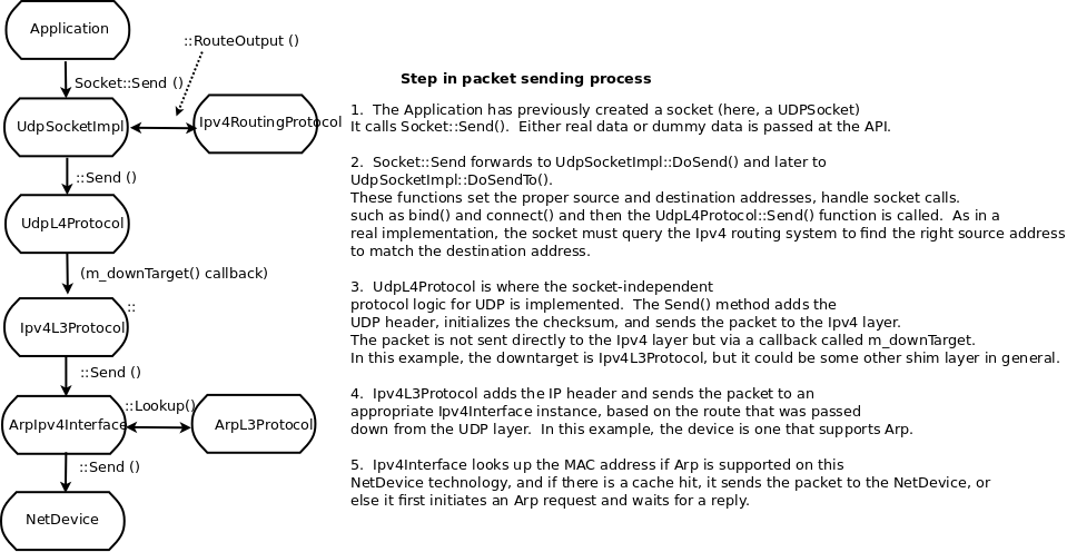
Send path of a packet.
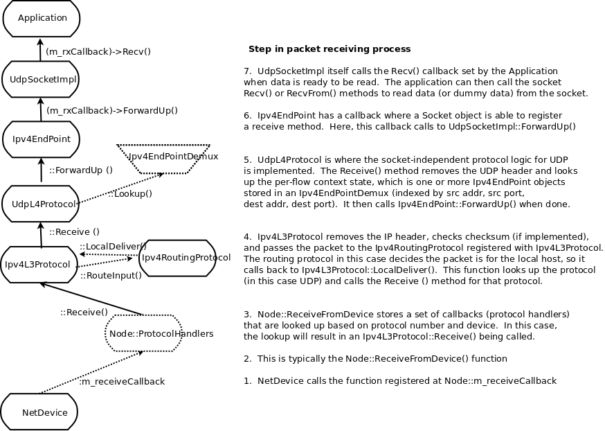
Receive path of a packet.
IPv4
This chapter describes the ns-3 IPv4 address assignment and basic components tracking.
IPv4 addresses assignment
In order to use IPv4 on a network, the first thing to do is assigning IPv4 addresses.
Any IPv4-enabled ns-3 node will have at least one NetDevice: the ns3::LoopbackNetDevice.
The loopback device address is 127.0.0.1.
All the other NetDevices will have one (or more) IPv4 addresses.
Note that, as today, ns-3 does not have a NAT module, and it does not follows the rules about filtering private addresses (RFC 1918): 10.0.0.0/8, 172.16.0.0/12, and 192.168.0.0/16. These addresses are routed as any other address. This behaviour could change in the future.
IPv4 global addresses can be:
- manually assigned
- assigned though DHCP
ns-3 can use both methods, and it’s quite important to understand the implications of both.
Manually assigned IPv4 addresses
This is probably the easiest and most used method. As an example:
Ptr<Node> n0 = CreateObject<Node> ();
Ptr<Node> n1 = CreateObject<Node> ();
NodeContainer net (n0, n1);
CsmaHelper csma;
NetDeviceContainer ndc = csma.Install (net);

NS_LOG_INFO ("Assign IPv4 Addresses.");
Ipv4AddressHelper ipv4;
ipv4.SetBase (Ipv4Address ("192.168.1.0"), NetMask ("/24"));
Ipv4InterfaceContainer ic = ipv4.Assign (ndc);
This method will add two global IPv4 addresses to the nodes.
Note that the addresses are assigned in sequence. As a consequence, the first Node / NetDevice will have “192.168.1.1”, the second “192.168.1.2” and so on.
It is possible to repeat the above to assign more than one address to a node.
However, due to the Ipv4AddressHelper singleton nature, one should first assign all the
addresses of a network, then change the network base (SetBase), then do a new assignment.
Alternatively, it is possible to assign a specific address to a node:
Ptr<Node> n0 = CreateObject<Node> ();
NodeContainer net (n0);
CsmaHelper csma;
NetDeviceContainer ndc = csma.Install (net);

NS_LOG_INFO ("Specifically Assign an IPv4 Address.");
Ipv4AddressHelper ipv4;
Ptr<NetDevice> device = ndc.Get (0);
Ptr<Node> node = device->GetNode ();
Ptr<Ipv4> ipv4proto = node->GetObject<Ipv4> ();
int32_t ifIndex = 0;
ifIndex = ipv4proto->GetInterfaceForDevice (device);
Ipv4InterfaceAddress ipv4Addr = Ipv4InterfaceAddress (Ipv4Address ("192.168.1.42"), NetMask ("/24"));
ipv4proto->AddAddress (ifIndex, ipv4Addr);
DHCP assigned IPv4 addresses
DHCP is available in the internet-apps module. In order to use DHCP you have to have a
DhcpServer application in a node (the DHC server node) and a DhcpClient application in
each of the nodes. Note that it not necessary that all the nodes in a subnet use DHCP. Some
nodes can have static addresses.
All the DHCP setup is performed though the DhcpHelper class. A complete example is in
src/internet-apps/examples/dhcp-example.cc.
Further info about the DHCP functionalities can be found in the internet-apps model documentation.
Tracing in the IPv4 Stack
The internet stack provides a number of trace sources in its various protocol implementations. These trace sources can be hooked using your own custom trace code, or you can use our helper functions in some cases to arrange for tracing to be enabled.
Tracing in ARP
ARP provides two trace hooks, one in the cache, and one in the layer three protocol. The trace accessor in the cache is given the name “Drop.” When a packet is transmitted over an interface that requires ARP, it is first queued for transmission in the ARP cache until the required MAC address is resolved. There are a number of retries that may be done trying to get the address, and if the maximum retry count is exceeded the packet in question is dropped by ARP. The single trace hook in the ARP cache is called,
- If an outbound packet is placed in the ARP cache pending address resolution and no resolution can be made within the maximum retry count, the outbound packet is dropped and this trace is fired;
A second trace hook lives in the ARP L3 protocol (also named “Drop”) and may be called for a number of reasons.
- If an ARP reply is received for an entry that is not waiting for a reply, the ARP reply packet is dropped and this trace is fired;
- If an ARP reply is received for a non-existent entry, the ARP reply packet is dropped and this trace is fired;
- If an ARP cache entry is in the DEAD state (has timed out) and an ARP reply packet is received, the reply packet is dropped and this trace is fired.
- Each ARP cache entry has a queue of pending packets. If the size of the queue is exceeded, the outbound packet is dropped and this trace is fired.
Tracing in IPv4
The IPv4 layer three protocol provides three trace hooks. These are the “Tx” (ns3::Ipv4L3Protocol::m_txTrace), “Rx” (ns3::Ipv4L3Protocol::m_rxTrace) and “Drop” (ns3::Ipv4L3Protocol::m_dropTrace) trace sources.
The “Tx” trace is fired in a number of situations, all of which indicate that a given packet is about to be sent down to a given ns3::Ipv4Interface.
- In the case of a packet destined for the broadcast address, the Ipv4InterfaceList is iterated and for every interface that is up and can fragment the packet or has a large enough MTU to transmit the packet, the trace is hit. See ns3::Ipv4L3Protocol::Send.
- In the case of a packet that needs routing, the “Tx” trace may be fired just before a packet is sent to the interface appropriate to the default gateway. See ns3::Ipv4L3Protocol::SendRealOut.
- Also in the case of a packet that needs routing, the “Tx” trace may be fired just before a packet is sent to the outgoing interface appropriate to the discovered route. See ns3::Ipv4L3Protocol::SendRealOut.
The “Rx” trace is fired when a packet is passed from the device up to the ns3::Ipv4L3Protocol::Receive function.
- In the receive function, the Ipv4InterfaceList is iterated, and if the Ipv4Interface corresponding to the receiving device is fount to be in the UP state, the trace is fired.
The “Drop” trace is fired in any case where the packet is dropped (in both the transmit and receive paths).
- In the ns3::Ipv4Interface::Receive function, the packet is dropped and the drop trace is hit if the interface corresponding to the receiving device is in the DOWN state.
- Also in the ns3::Ipv4Interface::Receive function, the packet is dropped and the drop trace is hit if the checksum is found to be bad.
- In ns3::Ipv4L3Protocol::Send, an outgoing packet bound for the broadcast address is dropped and the “Drop” trace is fired if the “don’t fragment” bit is set and fragmentation is available and required.
- Also in ns3::Ipv4L3Protocol::Send, an outgoing packet destined for the broadcast address is dropped and the “Drop” trace is hit if fragmentation is not available and is required (MTU < packet size).
- In the case of a broadcast address, an outgoing packet is cloned for each outgoing interface. If any of the interfaces is in the DOWN state, the “Drop” trace event fires with a reference to the copied packet.
- In the case of a packet requiring a route, an outgoing packet is dropped and the “Drop” trace event fires if no route to the remote host is found.
- In ns3::Ipv4L3Protocol::SendRealOut, an outgoing packet being routed is dropped and the “Drop” trace is fired if the “don’t fragment” bit is set and fragmentation is available and required.
- Also in ns3::Ipv4L3Protocol::SendRealOut, an outgoing packet being routed is dropped and the “Drop” trace is hit if fragmentation is not available and is required (MTU < packet size).
- An outgoing packet being routed is dropped and the “Drop” trace event fires if the required Ipv4Interface is in the DOWN state.
- If a packet is being forwarded, and the TTL is exceeded (see ns3::Ipv4L3Protocol::DoForward), the packet is dropped and the “Drop” trace event is fired.
Explicit Congestion Notification (ECN) bits
- In IPv4, ECN bits are the last 2 bits in TOS field and occupy 14th and 15th bits in the header.
- The IPv4 header class defines an EcnType enum with all four ECN codepoints (ECN_NotECT, ECN_ECT1, ECN_ECT0, ECN_CE) mentioned in RFC 3168, and also a setter and getter method to handle ECN values in the TOS field.
Ipv4QueueDiscItem
The traffic control sublayer in ns-3 handles objects of class
QueueDiscItem which are used to hold an ns3::Packet and an ns3::Header.
This is done to facilitate the marking of packets for Explicit
Congestion Notification. The Mark () method is implemented in
Ipv4QueueDiscItem. It returns true if marking the packet is successful, i.e.,
it successfully sets the CE bit in the IPv4 header. The Mark () method
will return false, however, if the IPv4 header indicates the ECN_NotECT
codepoint.
RFC 6621 duplicate packet detection
To support mesh network protocols over broadcast-capable networks (e.g. Wi-Fi),
it is useful to have support for duplicate packet detection and filtering,
since nodes in a network may receive multiple copies of flooded multicast
packets arriving on different paths. The Ipv4L3Protocol model in ns-3
has a model for hash-based duplicate packet detection (DPD) based on
Section 6.2.2 of (RFC 6621). The model, disabled by default, must be
enabled by setting EnableRFC6621 to true. A second attribute,
DuplicateExpire, sets the expiration delay for erasing the cache entry
of a packet in the duplicate cache; the delay value defaults to 1ms.
IPv6
This chapter describes the ns-3 IPv6 model capabilities and limitations along with its usage and examples.
IPv6 model description
The IPv6 model is loosely patterned after the Linux implementation; the implementation is not complete as some features of IPv6 are not of much interest to simulation studies, and some features of IPv6 are simply not modeled yet in ns-3.
The base class Ipv6
defines a generic API, while the class Ipv6L3Protocol is the actual class
implementing the protocol. The actual classes used by the IPv6 stack are located mainly
in the directory src/internet.
The implementation of IPv6 is contained in the following files:
src/internet/model/icmpv6-header.{cc,h}
src/internet/model/icmpv6-l4-protocol.{cc,h}
src/internet/model/ipv6.{cc,h}
src/internet/model/ipv6-address-generator.{cc,h}
src/internet/model/ipv6-autoconfigured-prefix.{cc,h}
src/internet/model/ipv6-end-point.{cc,h}
src/internet/model/ipv6-end-point-demux.{cc,h}
src/internet/model/ipv6-extension.{cc,h}
src/internet/model/ipv6-extension-demux.{cc,h}
src/internet/model/ipv6-extension-header.{cc,h}
src/internet/model/ipv6-header.{cc,h}
src/internet/model/ipv6-interface.{cc,h}
src/internet/model/ipv6-interface-address.{cc,h}
src/internet/model/ipv6-l3-protocol.{cc,h}
src/internet/model/ipv6-list-routing.{cc,h}
src/internet/model/ipv6-option.{cc,h}
src/internet/model/ipv6-option-demux.{cc,h}
src/internet/model/ipv6-option-header.{cc,h}
src/internet/model/ipv6-packet-info-tag.{cc,h}
src/internet/model/ipv6-pmtu-cache.{cc,h}
src/internet/model/ipv6-raw-socket-factory.{cc,h}
src/internet/model/ipv6-raw-socket-factory-impl.{cc,h}
src/internet/model/ipv6-raw-socket-impl.{cc,h}
src/internet/model/ipv6-route.{cc,h}
src/internet/model/ipv6-routing-protocol.{cc,h}
src/internet/model/ipv6-routing-table-entry.{cc,h}
src/internet/model/ipv6-static-routing.{cc,h}
src/internet/model/ndisc-cache.{cc,h}
src/network/utils/inet6-socket-address.{cc,h}
src/network/utils/ipv6-address.{cc,h}
Also some helpers are involved with IPv6:
src/internet/helper/internet-stack-helper.{cc,h}
src/internet/helper/ipv6-address-helper.{cc,h}
src/internet/helper/ipv6-interface-container.{cc,h}
src/internet/helper/ipv6-list-routing-helper.{cc,h}
src/internet/helper/ipv6-routing-helper.{cc,h}
src/internet/helper/ipv6-static-routing-helper.{cc,h}
The model files can be roughly divided into:
- protocol models (e.g., ipv6, ipv6-l3-protocol, icmpv6-l4-protocol, etc.)
- routing models (i.e., anything with ‘routing’ in its name)
- sockets and interfaces (e.g., ipv6-raw-socket, ipv6-interface, ipv6-end-point, etc.)
- address-related things
- headers, option headers, extension headers, etc.
- accessory classes (e.g., ndisc-cache)
Usage
The following description is based on using the typical helpers found in the example code.
IPv6 does not need to be activated in a node. it is automatically added to the available protocols once the Internet Stack is installed.
In order to not install IPv6 along with IPv4, it is possible to use
ns3::InternetStackHelper method SetIpv6StackInstall (bool enable)
before installing the InternetStack in the nodes.
Note that to have an IPv6-only network (i.e., to not install the IPv4 stack in a node)
one should use ns3::InternetStackHelper method SetIpv4StackInstall (bool enable)
before the stack installation.
As an example, in the following code node 0 will have both IPv4 and IPv6, node 1 only only IPv6 and node 2 only IPv4:
NodeContainer n;
n.Create (3);

InternetStackHelper internet;
InternetStackHelper internetV4only;
InternetStackHelper internetV6only;

internetV4only.SetIpv6StackInstall (false);
internetV6only.SetIpv4StackInstall (false);

internet.Install (n.Get (0));
internetV6only.Install (n.Get (1));
internetV4only.Install (n.Get (2));
IPv6 addresses assignment
In order to use IPv6 on a network, the first thing to do is assigning IPv6 addresses.
Any IPv6-enabled ns-3 node will have at least one NetDevice: the ns3::LoopbackNetDevice.
The loopback device address is ::1.
All the other NetDevices will have one or more IPv6 addresses:
- One link-local address:
fe80::interface ID, whereinterface IDis derived from the NetDevice MAC address. - Zero or more global addresses, e.g.,
2001:db8::1.
Typically the first address on an interface will be the link-local one, with the global address(es) being the following ones.
IPv6 global addresses might be:
- manually assigned
- auto-generated
ns-3 can use both methods, and it’s quite important to understand the implications of both.
Manually assigned IPv6 addresses
This is probably the easiest and most used method. As an example:
Ptr<Node> n0 = CreateObject<Node> ();
Ptr<Node> n1 = CreateObject<Node> ();
NodeContainer net (n0, n1);
CsmaHelper csma;
NetDeviceContainer ndc = csma.Install (net);

NS_LOG_INFO ("Assign IPv6 Addresses.");
Ipv6AddressHelper ipv6;
ipv6.SetBase (Ipv6Address ("2001:db8::"), Ipv6Prefix (64));
Ipv6InterfaceContainer ic = ipv6.Assign (ndc);
This method will add two global IPv6 addresses to the nodes. Note that, as usual for IPv6, all the nodes will also have a link-local address. Typically the first address on an interface will be the link-local one, with the global address(es) being the following ones.
Note that the global addresses will be derived from the MAC address. As a consequence, expect
to have addresses similar to 2001:db8::200:ff:fe00:1.
It is possible to repeat the above to assign more than one global address to a node.
However, due to the Ipv6AddressHelper singleton nature, one should first assign all the
addresses of a network, then change the network base (SetBase), then do a new assignment.
Alternatively, it is possible to assign a specific address to a node:
Ptr<Node> n0 = CreateObject<Node> ();
NodeContainer net (n0);
CsmaHelper csma;
NetDeviceContainer ndc = csma.Install (net);

NS_LOG_INFO ("Specifically Assign an IPv6 Address.");
Ipv6AddressHelper ipv6;
Ptr<NetDevice> device = ndc.Get (0);
Ptr<Node> node = device->GetNode ();
Ptr<Ipv6> ipv6proto = node->GetObject<Ipv6> ();
int32_t ifIndex = 0;
ifIndex = ipv6proto->GetInterfaceForDevice (device);
Ipv6InterfaceAddress ipv6Addr = Ipv6InterfaceAddress (Ipv6Address ("2001:db8:f00d:cafe::42"), Ipv6Prefix (64));
ipv6proto->AddAddress (ifIndex, ipv6Addr);
Auto-generated IPv6 addresses
This is accomplished by relying on the RADVD protocol, implemented by the class
Radvd. A helper class is available, which can be used to ease the most
common tasks, e.g., setting up a prefix on an interface, if it is announced periodically,
and if the router is the default router for that interface.
A fine grain configuration is possible though the RadvdInterface class, which
allows to setup every parameter of the announced router advertisement on a given interface.
It is worth mentioning that the configurations must be set up before installing the application in the node.
Upon using this method, the nodes will acquire dynamically (i.e., during the simulation) one (or more) global address(es) according to the RADVD configuration. These addresses will be bases on the RADVD announced prefix and the node’s EUI-64.
Examples of RADVD use are shown in examples/ipv6/radvd.cc
and examples/ipv6/radvd-two-prefix.cc.
Note that the router (i.e., the node with Radvd) will have to have a global address,
while the nodes using the auto-generated addresses (SLAAC) will have to have a link-local address.
This is accomplished using Ipv6AddressHelper::AssignWithoutAddress, e.g.:
Ipv6AddressHelper ipv6;
NetDeviceContainer tmp;
tmp.Add (d1.Get (0)); /* n0 */
Ipv6InterfaceContainer iic1 = ipv6.AssignWithoutAddress (tmp); /* n0 interface */
While IPv6 real nodes will use randomly generated addresses to protect privacy, ns-3 does NOT have this capability. This feature haven’t been so far considered as interesting for simulation.
Networks with and without the onlink property
IPv6 adds the concept of “on-link” for addresses and prefixes. Simplifying the concept, a network with the on-link property behaves roughly as IPv4: a node will assume that any address belonging to the on-link prefix is reachable on the link, so it uses Neighbor Discovery Protocol (NDP) to find the MAC address corresponding to the IPv6 address. If the prefix is not marked as “on-link”, then any packet is sent to the default router.
Radvd can announce prefixes that have the on-link flag not set. Moreover, it is possible
to add an address to a node without setting the on-link property for the prefix used in the address.
The function to use is Ipv6AddressHelper::AssignWithoutOnLink.
Duplicate Address Detection (DAD)
Nodes will perform DAD (it can be disabled using an Icmpv6L4Protocol attribute).
Upon receiving a DAD, however, nodes will not react to it. As is: DAD reaction is
incomplete so far.
The main reason relies on the missing random-generated address capability. Moreover,
since ns-3 nodes will usually be well-behaving, there shouldn’t be any Duplicate Address.
This might be changed in the future, so as to avoid issues with real-world
integrated simulations.
Explicit Congestion Notification (ECN) bits in IPv6
- In IPv6, ECN bits are the last 2 bits of the Traffic class and occupy 10th and 11th bit in the header.
- The IPv6 header class defines an EcnType enum with all four ECN codepoints (ECN_NotECT, ECN_ECT1, ECN_ECT0, ECN_CE) mentioned in RFC 3168, and also a setter and getter method to handle ECN values in the Traffic Class field.
Ipv6QueueDiscItem
The traffic control sublayer in ns-3 handles objects of class
QueueDiscItem which are used to hold an ns3::Packet and an ns3::Header.
This is done to facilitate the marking of packets for Explicit
Congestion Notification. The Mark () method is implemented in
Ipv6QueueDiscItem. It returns true if marking the packet is successful, i.e.,
it successfully sets the CE bit in the IPv6 header. The Mark () method
will return false, however, if the IPv6 header indicates the ECN_NotECT
codepoint.
Host and Router behaviour in IPv6 and ns-3
In IPv6 there is a clear distinction between routers and hosts. As one might expect, routers can forward packets from an interface to another interface, while hosts drop packets not directed to them.
Unfortunately, forwarding is not the only thing affected by this distinction, and forwarding itself might be fine-tuned, e.g., to forward packets incoming from an interface and drop packets from another interface.
In ns-3 a node is configured to be an host by default. There are two main ways to change this behaviour:
- Using
ns3::Ipv6InterfaceContainerSetForwarding(uint32_t i, bool router) whereiis the interface index in the container. - Changing the
ns3::Ipv6attributeIpForward.
Either one can be used during the simulation.
A fine-grained setup can be accomplished by using ns3::Ipv6Interface SetForwarding (bool forward);
which allows to change the behaviour on a per-interface-basis.
Note that the node-wide configuration only serves as a convenient method to enable/disable the
ns3::Ipv6Interface specific setting. An Ipv6Interface added to a node
with forwarding enabled will be set to be forwarding as well.
This is really important when a node has interfaces added during the simulation.
According to the ns3::Ipv6Interface forwarding state, the following happens:
- Forwarding OFF
- The node will NOT reply to Router Solicitation
- The node will react to Router Advertisement
- The node will periodically send Router Solicitation
- Routing protocols MUST DROP packets not directed to the node
- Forwarding ON
- The node will reply to Router Solicitation
- The node will NOT react to Router Advertisement
- The node will NOT send Router Solicitation
- Routing protocols MUST forward packets
The behaviour is matching ip-sysctl.txt (http://www.kernel.org/doc/Documentation/networking/ip-sysctl.txt) with the difference that it’s not possible to override the behaviour using esoteric settings (e.g., forwarding but accept router advertisements, accept_ra=2, or forwarding but send router solicitations forwarding=2).
Consider carefully the implications of packet forwarding. As an example, a node will NOT send ICMPv6 PACKET_TOO_BIG messages from an interface with forwarding off. This is completely normal, as the Routing protocol will drop the packet before attempting to forward it.
Helpers
Typically the helpers used in IPv6 setup are:
ns3::InternetStackHelperns3::Ipv6AddressHelperns3::Ipv6InterfaceContainer
The use is almost identical to the corresponding IPv4 case, e.g.:
NodeContainer n;
n.Create (4);

NS_LOG_INFO ("Create IPv6 Internet Stack");
InternetStackHelper internetv6;
internetv6.Install (n);

NS_LOG_INFO ("Create channels.");
CsmaHelper csma;
NetDeviceContainer d = csma.Install (n);

NS_LOG_INFO ("Create networks and assign IPv6 Addresses.");
Ipv6AddressHelper ipv6;
ipv6.SetBase (Ipv6Address ("2001:db8::"), Ipv6Prefix (64));
Ipv6InterfaceContainer iic = ipv6.Assign (d);
Additionally, a common task is to enable forwarding on one of the nodes and to setup a default route toward it in the other nodes, e.g.:
iic.SetForwarding (0, true);
iic.SetDefaultRouteInAllNodes (0);
This will enable forwarding on the node 0 and will setup a default route in
ns3::Ipv6StaticRouting on all the other nodes. Note that this
requires that Ipv6StaticRouting is present in the nodes.
The IPv6 routing helpers enable the user to perform specific tasks on the particular routing algorithm and to print the routing tables.
Attributes
Many classes in the ns-3 IPv6 implementation contain attributes. The most useful ones are:
ns3::Ipv6
- IpForward, boolean, default false. Globally enable or disable IP forwarding for all current and future IPv6 devices.
- MtuDiscover, boolean, default true. If disabled, every interface will have its MTU set to 1280 bytes.
ns3::Ipv6L3Protocol
- DefaultTtl, uint8_t, default 64. The TTL value set by default on all outgoing packets generated on this node.
- SendIcmpv6Redirect, boolean, default true. Send the ICMPv6 Redirect when appropriate.
ns3::Icmpv6L4Protocol
- DAD, boolean, default true. Always do DAD (Duplicate Address Detection) check.
ns3::NdiscCache
- UnresolvedQueueSize, uint32_t, default 3. Size of the queue for packets pending an NA reply.
Output
The IPv6 stack provides some useful trace sources:
ns3::Ipv6L3Protocol
- Tx, Send IPv6 packet to outgoing interface.
- Rx, Receive IPv6 packet from incoming interface.
- Drop, Drop IPv6 packet.
ns3::Ipv6Extension
- Drop, Drop IPv6 packet.
The latest trace source is generated when a packet contains an unknown option blocking its processing.
Mind that ns3::NdiscCache could drop packets as well, and they are not logged
in a trace source (yet). This might generate some confusion in the sent/received packets counters.
Advanced Usage
IPv6 maximum transmission unit (MTU) and fragmentation
ns-3 NetDevices define the MTU according to the L2 simulated Device. IPv6 requires that the minimum MTU is 1280 bytes, so all NetDevices are required to support at least this MTU. This is the link-MTU.
In order to support different MTUs in a source-destination path, ns-3 IPv6 model can perform fragmentation. This can be either triggered by receiving a packet bigger than the link-MTU from the L4 protocols (UDP, TCP, etc.), or by receiving an ICMPv6 PACKET_TOO_BIG message. The model mimics RFC 1981, with the following notable exceptions:
- L4 protocols are not informed of the Path MTU change
- TCP can not change its Segment Size according to the Path-MTU.
Both limitations are going to be removed in due time.
The Path-MTU cache is currently based on the source-destination IPv6 addresses. Further classifications (e.g., flow label) are possible but not yet implemented.
The Path-MTU default validity time is 10 minutes. After the cache entry expiration, the Path-MTU information is removed and the next packet will (eventually) trigger a new ICMPv6 PACKET_TOO_BIG message. Note that 1) this is consistent with the RFC specification and 2) L4 protocols are responsible for retransmitting the packets.
Examples
The examples for IPv6 are in the directory examples/ipv6. These examples focus on
the most interesting IPv6 peculiarities, such as fragmentation, redirect and so on.
Moreover, most TCP and UDP examples located in examples/udp, examples/tcp, etc.
have a command-line option to use IPv6 instead of IPv4.
Troubleshooting
There are just a few pitfalls to avoid while using ns-3 IPv6.
Routing loops
Since the only (so far) routing scheme available for IPv6 is ns3::Ipv6StaticRouting,
default router have to be setup manually. When there are two or more routers in a network
(e.g., node A and node B), avoid using the helper function SetDefaultRouteInAllNodes
for more than one router.
The consequence would be to install a default route to B in A and a default route pointing to A in B, generating a loop.
Global address leakage
Remember that addresses in IPv6 are global by definition. When using IPv6 with an emulation ns-3 capability, avoid at all costs address leakage toward the global Internet. It is advisable to setup an external firewall to prevent leakage.
2001:DB8::/32 addresses
IPv6 standard (RFC 3849) defines the 2001:DB8::/32 address class for the documentation.
This manual uses this convention. The addresses in this class are, however, only usable in
a document, and routers should discard them.
Validation
The IPv6 protocols has not yet been extensively validated against real implementations. The actual tests involve mainly performing checks of the .pcap trace files with Wireshark, and the results are positive.
Routing overview
ns-3 is intended to support traditional routing approaches and protocols, support ports of open source routing implementations, and facilitate research into unorthodox routing techniques. The overall routing architecture is described below in Routing architecture. Users who wish to just read about how to configure global routing for wired topologies can read Global centralized routing. Unicast routing protocols are described in Unicast routing. Multicast routing is documented in Multicast routing.
Routing architecture
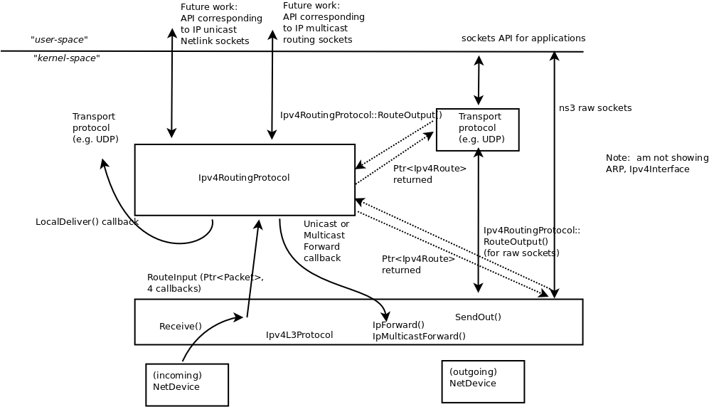
Overview of routing
Overview of routing shows the overall routing architecture for Ipv4. The key objects are Ipv4L3Protocol, Ipv4RoutingProtocol(s) (a class to which all routing/forwarding has been delegated from Ipv4L3Protocol), and Ipv4Route(s).
Ipv4L3Protocol must have at least one Ipv4RoutingProtocol added to it at simulation setup time. This is done explicitly by calling Ipv4::SetRoutingProtocol ().
The abstract base class Ipv4RoutingProtocol () declares a minimal interface, consisting of two methods: RouteOutput () and RouteInput (). For packets traveling outbound from a host, the transport protocol will query Ipv4 for the Ipv4RoutingProtocol object interface, and will request a route via Ipv4RoutingProtocol::RouteOutput (). A Ptr to Ipv4Route object is returned. This is analogous to a dst_cache entry in Linux. The Ipv4Route is carried down to the Ipv4L3Protocol to avoid a second lookup there. However, some cases (e.g. Ipv4 raw sockets) will require a call to RouteOutput() directly from Ipv4L3Protocol.
For packets received inbound for forwarding or delivery, the following steps occur. Ipv4L3Protocol::Receive() calls Ipv4RoutingProtocol::RouteInput(). This passes the packet ownership to the Ipv4RoutingProtocol object. There are four callbacks associated with this call:
- LocalDeliver
- UnicastForward
- MulticastForward
- Error
The Ipv4RoutingProtocol must eventually call one of these callbacks for each packet that it takes responsibility for. This is basically how the input routing process works in Linux.
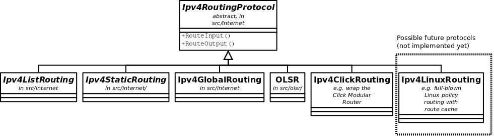
Ipv4Routing specialization.
This overall architecture is designed to support different routing approaches, including (in the future) a Linux-like policy-based routing implementation, proactive and on-demand routing protocols, and simple routing protocols for when the simulation user does not really care about routing.
Ipv4Routing specialization. illustrates how multiple routing protocols derive from this base class. A class Ipv4ListRouting (implementation class Ipv4ListRoutingImpl) provides the existing list routing approach in ns-3. Its API is the same as base class Ipv4Routing except for the ability to add multiple prioritized routing protocols (Ipv4ListRouting::AddRoutingProtocol(), Ipv4ListRouting::GetRoutingProtocol()).
The details of these routing protocols are described below in Unicast routing. For now, we will first start with a basic unicast routing capability that is intended to globally build routing tables at simulation time t=0 for simulation users who do not care about dynamic routing.
Unicast routing
The following unicast routing protocols are defined for IPv4 and IPv6:
- classes Ipv4ListRouting and Ipv6ListRouting (used to store a prioritized list of routing protocols)
- classes Ipv4StaticRouting and Ipv6StaticRouting (covering both unicast and multicast)
- class Ipv4GlobalRouting (used to store routes computed by the global route manager, if that is used)
- class Ipv4NixVectorRouting (a more efficient version of global routing that stores source routes in a packet header field)
- class Rip - the IPv4 RIPv2 protocol (RFC 2453)
- class RipNg - the IPv6 RIPng protocol (RFC 2080)
- IPv4 Optimized Link State Routing (OLSR) (a MANET protocol defined in RFC 3626)
- IPv4 Ad Hoc On Demand Distance Vector (AODV) (a MANET protocol defined in RFC 3561)
- IPv4 Destination Sequenced Distance Vector (DSDV) (a MANET protocol)
- IPv4 Dynamic Source Routing (DSR) (a MANET protocol)
In the future, this architecture should also allow someone to implement a Linux-like implementation with routing cache, or a Click modular router, but those are out of scope for now.
Ipv[4,6]ListRouting
This section describes the current default ns-3 Ipv[4,6]RoutingProtocol. Typically, multiple routing protocols are supported in user space and coordinate to write a single forwarding table in the kernel. Presently in ns-3, the implementation instead allows for multiple routing protocols to build/keep their own routing state, and the IP implementation will query each one of these routing protocols (in some order determined by the simulation author) until a route is found.
We chose this approach because it may better facilitate the integration of disparate routing approaches that may be difficult to coordinate the writing to a single table, approaches where more information than destination IP address (e.g., source routing) is used to determine the next hop, and on-demand routing approaches where packets must be cached.
Ipv[4,6]ListRouting::AddRoutingProtocol
Classes Ipv4ListRouting and Ipv6ListRouting provides a pure virtual function declaration for the method that allows one to add a routing protocol:
void AddRoutingProtocol (Ptr<Ipv4RoutingProtocol> routingProtocol,
                         int16_t priority);

void AddRoutingProtocol (Ptr<Ipv6RoutingProtocol> routingProtocol,
                         int16_t priority);
These methods are implemented respectively by class Ipv4ListRoutingImpl and by class Ipv6ListRoutingImpl in the internet module.
The priority variable above governs the priority in which the routing protocols are inserted. Notice that it is a signed int. By default in ns-3, the helper classes will instantiate a Ipv[4,6]ListRoutingImpl object, and add to it an Ipv[4,6]StaticRoutingImpl object at priority zero. Internally, a list of Ipv[4,6]RoutingProtocols is stored, and and the routing protocols are each consulted in decreasing order of priority to see whether a match is found. Therefore, if you want your Ipv4RoutingProtocol to have priority lower than the static routing, insert it with priority less than 0; e.g.:
Ptr<MyRoutingProtocol> myRoutingProto = CreateObject<MyRoutingProtocol> ();
listRoutingPtr->AddRoutingProtocol (myRoutingProto, -10);
Upon calls to RouteOutput() or RouteInput(), the list routing object will search the list of routing protocols, in priority order, until a route is found. Such routing protocol will invoke the appropriate callback and no further routing protocols will be searched.
Global centralized routing
Global centralized routing is sometimes called “God” routing; it is a special implementation that walks the simulation topology and runs a shortest path algorithm, and populates each node’s routing tables. No actual protocol overhead (on the simulated links) is incurred with this approach. It does have a few constraints:
- Wired only: It is not intended for use in wireless networks.
- Unicast only: It does not do multicast.
- Scalability: Some users of this on large topologies (e.g. 1000 nodes) have noticed that the current implementation is not very scalable. The global centralized routing will be modified in the future to reduce computations and runtime performance.
Presently, global centralized IPv4 unicast routing over both point-to-point and shared (CSMA) links is supported.
By default, when using the ns-3 helper API and the default InternetStackHelper, global routing capability will be added to the node, and global routing will be inserted as a routing protocol with lower priority than the static routes (i.e., users can insert routes via Ipv4StaticRouting API and they will take precedence over routes found by global routing).
Global Unicast Routing API
The public API is very minimal. User scripts include the following:
#include "ns3/internet-module.h"
If the default InternetStackHelper is used, then an instance of global routing will be aggregated to each node. After IP addresses are configured, the following function call will cause all of the nodes that have an Ipv4 interface to receive forwarding tables entered automatically by the GlobalRouteManager:
Ipv4GlobalRoutingHelper::PopulateRoutingTables ();
Note: A reminder that the wifi NetDevice will work but does not take any wireless effects into account. For wireless, we recommend OLSR dynamic routing described below.
It is possible to call this function again in the midst of a simulation using the following additional public function:
Ipv4GlobalRoutingHelper::RecomputeRoutingTables ();
which flushes the old tables, queries the nodes for new interface information, and rebuilds the routes.
For instance, this scheduling call will cause the tables to be rebuilt at time 5 seconds:
Simulator::Schedule (Seconds (5),
                     &Ipv4GlobalRoutingHelper::RecomputeRoutingTables);
There are two attributes that govern the behavior. The first is Ipv4GlobalRouting::RandomEcmpRouting. If set to true, packets are randomly routed across equal-cost multipath routes. If set to false (default), only one route is consistently used. The second is Ipv4GlobalRouting::RespondToInterfaceEvents. If set to true, dynamically recompute the global routes upon Interface notification events (up/down, or add/remove address). If set to false (default), routing may break unless the user manually calls RecomputeRoutingTables() after such events. The default is set to false to preserve legacy ns-3 program behavior.
Global Routing Implementation
This section is for those readers who care about how this is implemented. A singleton object (GlobalRouteManager) is responsible for populating the static routes on each node, using the public Ipv4 API of that node. It queries each node in the topology for a “globalRouter” interface. If found, it uses the API of that interface to obtain a “link state advertisement (LSA)” for the router. Link State Advertisements are used in OSPF routing, and we follow their formatting.
It is important to note that all of these computations are done before packets are flowing in the network. In particular, there are no overhead or control packets being exchanged when using this implementation. Instead, this global route manager just walks the list of nodes to build the necessary information and configure each node’s routing table.
The GlobalRouteManager populates a link state database with LSAs gathered from the entire topology. Then, for each router in the topology, the GlobalRouteManager executes the OSPF shortest path first (SPF) computation on the database, and populates the routing tables on each node.
The quagga (http://www.quagga.net) OSPF implementation was used as the basis for the routing computation logic. One benefit of following an existing OSPF SPF implementation is that OSPF already has defined link state advertisements for all common types of network links:
- point-to-point (serial links)
- point-to-multipoint (Frame Relay, ad hoc wireless)
- non-broadcast multiple access (ATM)
- broadcast (Ethernet)
Therefore, we think that enabling these other link types will be more straightforward now that the underlying OSPF SPF framework is in place.
Presently, we can handle IPv4 point-to-point, numbered links, as well as shared broadcast (CSMA) links. Equal-cost multipath is also supported. Although wireless link types are supported by the implementation, note that due to the nature of this implementation, any channel effects will not be considered and the routing tables will assume that every node on the same shared channel is reachable from every other node (i.e. it will be treated like a broadcast CSMA link).
The GlobalRouteManager first walks the list of nodes and aggregates a GlobalRouter interface to each one as follows:
typedef std::vector < Ptr<Node> >::iterator Iterator;
for (Iterator i = NodeList::Begin (); i != NodeList::End (); i++)
  {
    Ptr<Node> node = *i;
    Ptr<GlobalRouter> globalRouter = CreateObject<GlobalRouter> (node);
    node->AggregateObject (globalRouter);
  }
This interface is later queried and used to generate a Link State Advertisement for each router, and this link state database is fed into the OSPF shortest path computation logic. The Ipv4 API is finally used to populate the routes themselves.
RIP and RIPng
The RIPv2 protocol for IPv4 is described in the RFC 2453, and it consolidates a number of improvements over the base protocol defined in RFC 1058.
This IPv6 routing protocol (RFC 2080) is the evolution of the well-known RIPv1 (see RFC 1058 and RFC 1723) routing protocol for IPv4.
The protocols are very simple, and are normally suitable for flat, simple network topologies.
RIPv1, RIPv2, and RIPng have the very same goals and limitations. In particular, RIP considers any route with a metric equal or greater than 16 as unreachable. As a consequence, the maximum number of hops is the network must be less than 15 (the number of routers is not set). Users are encouraged to read RFC 2080 and RFC 1058 to fully understand RIP behaviour and limitations.
Routing convergence
RIP uses a Distance-Vector algorithm, and routes are updated according to the Bellman-Ford algorithm (sometimes known as Ford-Fulkerson algorithm). The algorithm has a convergence time of O(|V|*|E|) where |V| and |E| are the number of vertices (routers) and edges (links) respectively. It should be stressed that the convergence time is the number of steps in the algorithm, and each step is triggered by a message. Since Triggered Updates (i.e., when a route is changed) have a 1-5 seconds cooldown, the topology can require some time to be stabilized.
Users should be aware that, during routing tables construction, the routers might drop packets. Data traffic should be sent only after a time long enough to allow RIP to build the network topology. Usually 80 seconds should be enough to have a suboptimal (but working) routing setup. This includes the time needed to propagate the routes to the most distant router (16 hops) with Triggered Updates.
If the network topology is changed (e.g., a link is broken), the recovery time might be quite high, and it might be even higher than the initial setup time. Moreover, the network topology recovery is affected by the Split Horizoning strategy.
The examples examples/routing/ripng-simple-network.cc and
examples/routing/rip-simple-network.cc
shows both the network setup and network recovery phases.
Split Horizoning
Split Horizon is a strategy to prevent routing instability. Three options are possible:
- No Split Horizon
- Split Horizon
- Poison Reverse
In the first case, routes are advertised on all the router’s interfaces. In the second case, routers will not advertise a route on the interface from which it was learned. Poison Reverse will advertise the route on the interface from which it was learned, but with a metric of 16 (infinity). For a full analysis of the three techniques, see RFC 1058, section 2.2.
The examples are based on the network topology described in the RFC, but it does not show the effect described there.
The reason are the Triggered Updates, together with the fact that when a router invalidates a route, it will immediately propagate the route unreachability, thus preventing most of the issues described in the RFC.
However, with complex topologies, it is still possible to have route instability phenomena similar to the one described in the RFC after a link failure. As a consequence, all the considerations about Split Horizon remains valid.
Default routes
RIP protocol should be installed only on routers. As a consequence, nodes will not know what is the default router.
To overcome this limitation, users should either install the default route manually (e.g., by resorting to Ipv4StaticRouting or Ipv6StaticRouting), or by using RADVd (in case of IPv6). RADVd is available in ns-3 in the Applications module, and it is strongly suggested.
Protocol parameters and options
The RIP ns-3 implementations allow to change all the timers associated with route updates and routes lifetime.
Moreover, users can change the interface metrics on a per-node basis.
The type of Split Horizoning (to avoid routes back-propagation) can be selected on a per-node basis, with the choices being “no split horizon”, “split horizon” and “poison reverse”. See RFC 2080 for further details, and RFC 1058 for a complete discussion on the split horizoning strategies.
Moreover, it is possible to use a non-standard value for Link Down Value (i.e., the value after which a link is considered down). The default is value is 16.
Limitations
There is no support for the Next Hop option (RFC 2080, Section 2.1.1). The Next Hop option is useful when RIP is not being run on all of the routers on a network. Support for this option may be considered in the future.
There is no support for CIDR prefix aggregation. As a result, both routing tables and route advertisements may be larger than necessary. Prefix aggregation may be added in the future.
Other routing protocols
Other routing protocols documentation can be found under the respective modules sections, e.g.:
- AODV
- Click
- DSDV
- DSR
- NixVectorRouting
- OLSR
- etc.
Multicast routing
The following function is used to add a static multicast route to a node:
void
Ipv4StaticRouting::AddMulticastRoute (Ipv4Address origin,
                                      Ipv4Address group,
                                      uint32_t inputInterface,
                                      std::vector<uint32_t> outputInterfaces);
A multicast route must specify an origin IP address, a multicast group and an input network interface index as conditions and provide a vector of output network interface indices over which packets matching the conditions are sent.
Typically there are two main types of multicast routes:
- Routes used during forwarding, and
- Routes used in the originator node.
In the first case all the conditions must be explicitly provided.
In the second case, the route is equivalent to a unicast route, and must be added through Ipv4StaticRouting::AddHostRouteTo.
Another command sets the default multicast route:
void
Ipv4StaticRouting::SetDefaultMulticastRoute (uint32_t outputInterface);
This is the multicast equivalent of the unicast version SetDefaultRoute. We tell the routing system what to do in the case where a specific route to a destination multicast group is not found. The system forwards packets out the specified interface in the hope that “something out there” knows better how to route the packet. This method is only used in initially sending packets off of a host. The default multicast route is not consulted during forwarding – exact routes must be specified using AddMulticastRoute for that case.
Since we’re basically sending packets to some entity we think may know better what to do, we don’t pay attention to “subtleties” like origin address, nor do we worry about forwarding out multiple interfaces. If the default multicast route is set, it is returned as the selected route from LookupStatic irrespective of origin or multicast group if another specific route is not found.
Finally, a number of additional functions are provided to fetch and remove multicast routes:
uint32_t GetNMulticastRoutes (void) const;

Ipv4MulticastRoute *GetMulticastRoute (uint32_t i) const;

Ipv4MulticastRoute *GetDefaultMulticastRoute (void) const;

bool RemoveMulticastRoute (Ipv4Address origin,
                           Ipv4Address group,
                           uint32_t inputInterface);

void RemoveMulticastRoute (uint32_t index);
TCP models in ns-3
This chapter describes the TCP models available in ns-3.
Overview of support for TCP
ns-3 was written to support multiple TCP implementations. The implementations
inherit from a few common header classes in the src/network directory, so that
user code can swap out implementations with minimal changes to the scripts.
There are three important abstract base classes:
- class
TcpSocket: This is defined insrc/internet/model/tcp-socket.{cc,h}. This class exists for hosting TcpSocket attributes that can be reused across different implementations. For instance, the attributeInitialCwndcan be used for any of the implementations that derive from classTcpSocket. - class
TcpSocketFactory: This is used by the layer-4 protocol instance to create TCP sockets of the right type. - class
TcpCongestionOps: This supports different variants of congestion control– a key topic of simulation-based TCP research.
There are presently two active and one legacy implementations of TCP available for ns-3.
- a natively implemented TCP for ns-3
- support for kernel implementations via Direct Code Execution (DCE)
- (legacy) support for kernel implementations for the Network Simulation Cradle (NSC)
NSC is no longer actively supported; it requires use of gcc-5 or gcc-4.9, and only covers up to Linux kernel version 2.6.29.
Direct Code Execution is also limited in its support for newer kernels; at present, only Linux kernel 4.4 is supported. However, the TCP implementations in kernel 4.4 can still be used for ns-3 validation or for specialized simulation use cases.
It should also be mentioned that various ways of combining virtual machines with ns-3 makes available also some additional TCP implementations, but those are out of scope for this chapter.
ns-3 TCP
In brief, the native ns-3 TCP model supports a full bidirectional TCP with connection setup and close logic. Several congestion control algorithms are supported, with CUBIC the default, and NewReno, Westwood, Hybla, HighSpeed, Vegas, Scalable, Veno, Binary Increase Congestion Control (BIC), Yet Another HighSpeed TCP (YeAH), Illinois, H-TCP, Low Extra Delay Background Transport (LEDBAT), TCP Low Priority (TCP-LP), Data Center TCP (DCTCP) and Bottleneck Bandwidth and RTT (BBR) also supported. The model also supports Selective Acknowledgements (SACK), Proportional Rate Reduction (PRR) and Explicit Congestion Notification (ECN). Multipath-TCP is not yet supported in the ns-3 releases.
Model history
Until the ns-3.10 release, ns-3 contained a port of the TCP model from GTNetS, developed initially by George Riley and ported to ns-3 by Raj Bhattacharjea. This implementation was substantially rewritten by Adriam Tam for ns-3.10. In 2015, the TCP module was redesigned in order to create a better environment for creating and carrying out automated tests. One of the main changes involves congestion control algorithms, and how they are implemented.
Before the ns-3.25 release, a congestion control was considered as a stand-alone TCP
through an inheritance relation: each congestion control (e.g. TcpNewReno) was
a subclass of TcpSocketBase, reimplementing some inherited methods. The
architecture was redone to avoid this inheritance,
by making each congestion control a separate class, and defining an interface
to exchange important data between TcpSocketBase and the congestion modules.
The Linux tcp_congestion_ops interface was used as the design reference.
Along with congestion control, Fast Retransmit and Fast Recovery algorithms have been modified; in previous releases, these algorithms were delegated to TcpSocketBase subclasses. Starting from ns-3.25, they have been merged inside TcpSocketBase. In future releases, they can be extracted as separate modules, following the congestion control design.
As of the ns-3.31 release, the default initial window was set to 10 segments (in previous releases, it was set to 1 segment). This aligns with current Linux default, and is discussed further in RFC 6928.
In the ns-3.32 release, the default recovery algorithm was set to Proportional Rate Reduction (PRR) from the classic ack-clocked Fast Recovery algorithm.
In the ns-3.34 release, the default congestion control algorithm was set to CUBIC from NewReno.
Acknowledgments
As mentioned above, ns-3 TCP has had multiple authors and maintainers over the years. Several publications exist on aspects of ns-3 TCP, and users of ns-3 TCP are requested to cite one of the applicable papers when publishing new work.
A general reference on the current architecture is found in the following paper:
- Maurizio Casoni, Natale Patriciello, Next-generation TCP for ns-3 simulator, Simulation Modelling Practice and Theory, Volume 66, 2016, Pages 81-93. (http://www.sciencedirect.com/science/article/pii/S1569190X15300939)
For an academic peer-reviewed paper on the SACK implementation in ns-3, please refer to:
- Natale Patriciello. 2017. A SACK-based Conservative Loss Recovery Algorithm for ns-3 TCP: a Linux-inspired Proposal. In Proceedings of the Workshop on ns-3 (WNS3 ‘17). ACM, New York, NY, USA, 1-8. (https://dl.acm.org/citation.cfm?id=3067666)
Usage
In many cases, usage of TCP is set at the application layer by telling the ns-3 application which kind of socket factory to use.
Using the helper functions defined in src/applications/helper and
src/network/helper, here is how one would create a TCP receiver:
// Create a packet sink on the star "hub" to receive these packets
uint16_t port = 50000;
Address sinkLocalAddress(InetSocketAddress (Ipv4Address::GetAny (), port));
PacketSinkHelper sinkHelper ("ns3::TcpSocketFactory", sinkLocalAddress);
ApplicationContainer sinkApp = sinkHelper.Install (serverNode);
sinkApp.Start (Seconds (1.0));
sinkApp.Stop (Seconds (10.0));
Similarly, the below snippet configures OnOffApplication traffic source to use TCP:
// Create the OnOff applications to send TCP to the server
OnOffHelper clientHelper ("ns3::TcpSocketFactory", Address ());
The careful reader will note above that we have specified the TypeId of an
abstract base class TcpSocketFactory. How does the script tell
ns-3 that it wants the native ns-3 TCP vs. some other one? Well, when
internet stacks are added to the node, the default TCP implementation that is
aggregated to the node is the ns-3 TCP. This can be overridden as we show
below when using Network Simulation Cradle. So, by default, when using the ns-3
helper API, the TCP that is aggregated to nodes with an Internet stack is the
native ns-3 TCP.
To configure behavior of TCP, a number of parameters are exported through the
ns-3 attribute system. These are documented in the Doxygen for class
TcpSocket. For example, the maximum segment size is a
settable attribute.
To set the default socket type before any internet stack-related objects are created, one may put the following statement at the top of the simulation program:
Config::SetDefault ("ns3::TcpL4Protocol::SocketType", StringValue ("ns3::TcpNewReno"));
For users who wish to have a pointer to the actual socket (so that
socket operations like Bind(), setting socket options, etc. can be
done on a per-socket basis), Tcp sockets can be created by using the
Socket::CreateSocket() method. The TypeId passed to CreateSocket()
must be of type ns3::SocketFactory, so configuring the underlying
socket type must be done by twiddling the attribute associated with the
underlying TcpL4Protocol object. The easiest way to get at this would be
through the attribute configuration system. In the below example,
the Node container “n0n1” is accessed to get the zeroth element, and a socket is
created on this node:
// Create and bind the socket...
TypeId tid = TypeId::LookupByName ("ns3::TcpNewReno");
Config::Set ("/NodeList/*/$ns3::TcpL4Protocol/SocketType", TypeIdValue (tid));
Ptr<Socket> localSocket =
  Socket::CreateSocket (n0n1.Get (0), TcpSocketFactory::GetTypeId ());
Above, the “*” wild card for node number is passed to the attribute configuration system, so that all future sockets on all nodes are set to NewReno, not just on node ‘n0n1.Get (0)’. If one wants to limit it to just the specified node, one would have to do something like:
// Create and bind the socket...
TypeId tid = TypeId::LookupByName ("ns3::TcpNewReno");
std::stringstream nodeId;
nodeId << n0n1.Get (0)->GetId ();
std::string specificNode = "/NodeList/" + nodeId.str () + "/$ns3::TcpL4Protocol/SocketType";
Config::Set (specificNode, TypeIdValue (tid));
Ptr<Socket> localSocket =
  Socket::CreateSocket (n0n1.Get (0), TcpSocketFactory::GetTypeId ());
Once a TCP socket is created, one will want to follow conventional socket logic and either connect() and send() (for a TCP client) or bind(), listen(), and accept() (for a TCP server). Please note that applications usually create the sockets they use automatically, and so is not straightforward to connect directly to them using pointers. Please refer to the source code of your preferred application to discover how and when it creates the socket.
TCP Socket interaction and interface with Application layer
In the following there is an analysis on the public interface of the TCP socket, and how it can be used to interact with the socket itself. An analysis of the callback fired by the socket is also carried out. Please note that, for the sake of clarity, we will use the terminology “Sender” and “Receiver” to clearly divide the functionality of the socket. However, in TCP these two roles can be applied at the same time (i.e. a socket could be a sender and a receiver at the same time): our distinction does not lose generality, since the following definition can be applied to both sockets in case of full-duplex mode.
TCP state machine (for commodity use)
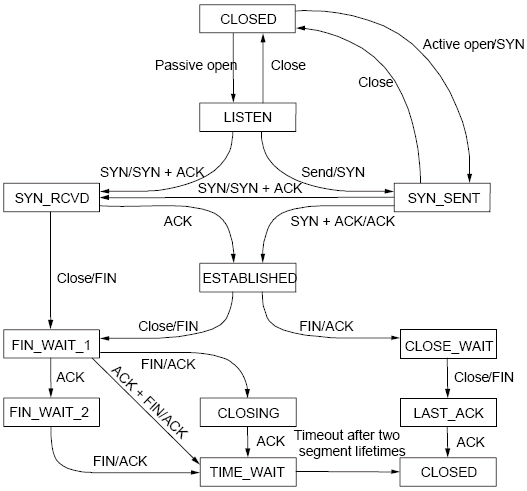
TCP State machine
In ns-3 we are fully compliant with the state machine depicted in Figure TCP State machine.
Public interface for receivers (e.g. servers receiving data)
- Bind()
- Bind the socket to an address, or to a general endpoint. A general endpoint is an endpoint with an ephemeral port allocation (that is, a random port allocation) on the 0.0.0.0 IP address. For instance, in current applications, data senders usually binds automatically after a Connect() over a random port. Consequently, the connection will start from this random port towards the well-defined port of the receiver. The IP 0.0.0.0 is then translated by lower layers into the real IP of the device.
- Bind6()
- Same as Bind(), but for IPv6.
- BindToNetDevice()
- Bind the socket to the specified NetDevice, creating a general endpoint.
- Listen()
- Listen on the endpoint for an incoming connection. Please note that this function can be called only in the TCP CLOSED state, and transit in the LISTEN state. When an incoming request for connection is detected (i.e. the other peer invoked Connect()) the application will be signaled with the callback NotifyConnectionRequest (set in SetAcceptCallback() beforehand). If the connection is accepted (the default behavior, when the associated callback is a null one) the Socket will fork itself, i.e. a new socket is created to handle the incoming data/connection, in the state SYN_RCVD. Please note that this newly created socket is not connected anymore to the callbacks on the “father” socket (e.g. DataSent, Recv); the pointer of the newly created socket is provided in the Callback NotifyNewConnectionCreated (set beforehand in SetAcceptCallback), and should be used to connect new callbacks to interesting events (e.g. Recv callback). After receiving the ACK of the SYN-ACK, the socket will set the congestion control, move into ESTABLISHED state, and then notify the application with NotifyNewConnectionCreated.
- ShutdownSend()
- Signal a termination of send, or in other words prevents data from being added to the buffer. After this call, if buffer is already empty, the socket will send a FIN, otherwise FIN will go when buffer empties. Please note that this is useful only for modeling “Sink” applications. If you have data to transmit, please refer to the Send() / Close() combination of API.
- GetRxAvailable()
- Get the amount of data that could be returned by the Socket in one or multiple call to Recv or RecvFrom. Please use the Attribute system to configure the maximum available space on the receiver buffer (property “RcvBufSize”).
- Recv()
- Grab data from the TCP socket. Please remember that TCP is a stream socket, and it is allowed to concatenate multiple packets into bigger ones. If no data is present (i.e. GetRxAvailable returns 0) an empty packet is returned. Set the callback RecvCallback through SetRecvCallback() in order to have the application automatically notified when some data is ready to be read. It’s important to connect that callback to the newly created socket in case of forks.
- RecvFrom()
- Same as Recv, but with the source address as parameter.
Public interface for senders (e.g. clients uploading data)
- Connect()
- Set the remote endpoint, and try to connect to it. The local endpoint should be set before this call, or otherwise an ephemeral one will be created. The TCP then will be in the SYN_SENT state. If a SYN-ACK is received, the TCP will setup the congestion control, and then call the callback ConnectionSucceeded.
- GetTxAvailable()
- Return the amount of data that can be stored in the TCP Tx buffer. Set this property through the Attribute system (“SndBufSize”).
- Send()
- Send the data into the TCP Tx buffer. From there, the TCP rules will decide if, and when, this data will be transmitted. Please note that, if the tx buffer has enough data to fill the congestion (or the receiver) window, dynamically varying the rate at which data is injected in the TCP buffer does not have any noticeable effect on the amount of data transmitted on the wire, that will continue to be decided by the TCP rules.
- SendTo()
- Same as Send().
- Close()
- Terminate the local side of the connection, by sending a FIN (after all data in the tx buffer has been transmitted). This does not prevent the socket in receiving data, and employing retransmit mechanism if losses are detected. If the application calls Close() with unread data in its rx buffer, the socket will send a reset. If the socket is in the state SYN_SENT, CLOSING, LISTEN, FIN_WAIT_2, or LAST_ACK, after that call the application will be notified with NotifyNormalClose(). In other cases, the notification is delayed (see NotifyNormalClose()).
Public callbacks
These callbacks are called by the TCP socket to notify the application of interesting events. We will refer to these with the protected name used in socket.h, but we will provide the API function to set the pointers to these callback as well.
- NotifyConnectionSucceeded: SetConnectCallback, 1st argument
- Called in the SYN_SENT state, before moving to ESTABLISHED. In other words, we have sent the SYN, and we received the SYN-ACK: the socket prepares the sequence numbers, sends the ACK for the SYN-ACK, tries to send out more data (in another segment) and then invokes this callback. After this callback, it invokes the NotifySend callback.
- NotifyConnectionFailed: SetConnectCallback, 2nd argument
- Called after the SYN retransmission count goes to 0. SYN packet is lost multiple times, and the socket gives up.
- NotifyNormalClose: SetCloseCallbacks, 1st argument
- A normal close is invoked. A rare case is when we receive an RST segment (or a segment with bad flags) in normal states. All other cases are: - The application tries to Connect() over an already connected socket - Received an ACK for the FIN sent, with or without the FIN bit set (we are in LAST_ACK) - The socket reaches the maximum amount of retries in retransmitting the SYN (*) - We receive a timeout in the LAST_ACK state - Upon entering the TIME_WAIT state, before waiting the 2*Maximum Segment Lifetime seconds to finally deallocate the socket.
- NotifyErrorClose: SetCloseCallbacks, 2nd argument
- Invoked when we send an RST segment (for whatever reason) or we reached the maximum amount of data retries.
- NotifyConnectionRequest: SetAcceptCallback, 1st argument
- Invoked in the LISTEN state, when we receive a SYN. The return value indicates if the socket should accept the connection (return true) or should ignore it (return false).
- NotifyNewConnectionCreated: SetAcceptCallback, 2nd argument
- Invoked when from SYN_RCVD the socket passes to ESTABLISHED, and after setting up the congestion control, the sequence numbers, and processing the incoming ACK. If there is some space in the buffer, NotifySend is called shortly after this callback. The Socket pointer, passed with this callback, is the newly created socket, after a Fork().
- NotifyDataSent: SetDataSentCallback
- The Socket notifies the application that some bytes have been transmitted on the IP level. These bytes could still be lost in the node (traffic control layer) or in the network.
- NotifySend: SetSendCallback
- Invoked if there is some space in the tx buffer when entering the ESTABLISHED state (e.g. after the ACK for SYN-ACK is received), after the connection succeeds (e.g. after the SYN-ACK is received) and after each new ACK (i.e. that advances SND.UNA).
- NotifyDataRecv: SetRecvCallback
- Called when in the receiver buffer there are in-order bytes, and when in FIN_WAIT_1 or FIN_WAIT_2 the socket receive a in-sequence FIN (that can carry data).
Congestion Control Algorithms
Here follows a list of supported TCP congestion control algorithms. For an academic paper on many of these congestion control algorithms, see http://dl.acm.org/citation.cfm?id=2756518 .
NewReno
NewReno algorithm introduces partial ACKs inside the well-established Reno algorithm. This and other modifications are described in RFC 6582. We have two possible congestion window increment strategy: slow start and congestion avoidance. Taken from RFC 5681:
During slow start, a TCP increments cwnd by at most SMSS bytes for each ACK received that cumulatively acknowledges new data. Slow start ends when cwnd exceeds ssthresh (or, optionally, when it reaches it, as noted above) or when congestion is observed. While traditionally TCP implementations have increased cwnd by precisely SMSS bytes upon receipt of an ACK covering new data, we RECOMMEND that TCP implementations increase cwnd, per Equation (1), where N is the number of previously unacknowledged bytes acknowledged in the incoming ACK.
(1)
During congestion avoidance, cwnd is incremented by roughly 1 full-sized segment per round-trip time (RTT), and for each congestion event, the slow start threshold is halved.
CUBIC
CUBIC (class TcpCubic) is the default TCP congestion control
in Linux, macOS (since 2014), and Microsoft Windows (since 2017).
CUBIC has two main differences with respect to
a more classic TCP congestion control such as NewReno. First, during the
congestion avoidance phase, the window size grows according to a cubic
function (concave, then convex) with the latter convex portion designed
to allow for bandwidth probing. Second, a hybrid slow start (HyStart)
algorithm uses observations of delay increases in the slow start
phase of window growth to try to exit slow start before window growth
causes queue overflow.
CUBIC is documented in RFC 8312, and the ns-3 implementation is based on the RFC more so than the Linux implementation, although the Linux 4.4 kernel implementation (through the Direct Code Execution environment) has been used to validate the behavior and is fairly well aligned (see below section on validation).
Linux Reno
TCP Linux Reno (class TcpLinuxReno) is designed to provide a
Linux-like implementation of
TCP NewReno. The implementation of class TcpNewReno in ns-3
follows RFC standards, and increases cwnd more conservatively than does Linux Reno.
Linux Reno modifies slow start and congestion avoidance algorithms to
increase cwnd based on the number of bytes being acknowledged by each
arriving ACK, rather than by the number of ACKs that arrive. Another major
difference in implementation is that Linux maintains the congestion window
in units of segments, while the RFCs define the congestion window in units of
bytes.
In slow start phase, on each incoming ACK at the TCP sender side cwnd is increased by the number of previously unacknowledged bytes ACKed by the incoming acknowledgment. In contrast, in ns-3 NewReno, cwnd is increased by one segment per acknowledgment. In standards terminology, this difference is referred to as Appropriate Byte Counting (RFC 3465); Linux follows Appropriate Byte Counting while ns-3 NewReno does not.
(2)
(3)
In congestion avoidance phase, the number of bytes that have been ACKed at the TCP sender side are stored in a ‘bytes_acked’ variable in the TCP control block. When ‘bytes_acked’ becomes greater than or equal to the value of the cwnd, ‘bytes_acked’ is reduced by the value of cwnd. Next, cwnd is incremented by a full-sized segment (SMSS). In contrast, in ns-3 NewReno, cwnd is increased by (1/cwnd) with a rounding off due to type casting into int.
if (m_cWndCnt >= w)
 {
   uint32_t delta = m_cWndCnt / w;

   m_cWndCnt -= delta * w;
   tcb->m_cWnd += delta * tcb->m_segmentSize;
   NS_LOG_DEBUG ("Subtracting delta * w from m_cWndCnt " << delta * w);
 }

:label: linuxrenocongavoid
if (segmentsAcked > 0)
 {
   double adder = static_cast<double> (tcb->m_segmentSize * tcb->m_segmentSize) / tcb->m_cWnd.Get ();
   adder = std::max (1.0, adder);
   tcb->m_cWnd += static_cast<uint32_t> (adder);
   NS_LOG_INFO ("In CongAvoid, updated to cwnd " << tcb->m_cWnd <<
                " ssthresh " << tcb->m_ssThresh);
 }

:label: newrenocongavoid
So, there are two main difference between the TCP Linux Reno and TCP NewReno in ns-3: 1) In TCP Linux Reno, delayed acknowledgement configuration does not affect congestion window growth, while in TCP NewReno, delayed acknowledgments cause a slower congestion window growth. 2) In congestion avoidance phase, the arithmetic for counting the number of segments acked and deciding when to increment the cwnd is different for TCP Linux Reno and TCP NewReno.
Following graphs shows the behavior of window growth in TCP Linux Reno and TCP NewReno with delayed acknowledgement of 2 segments:
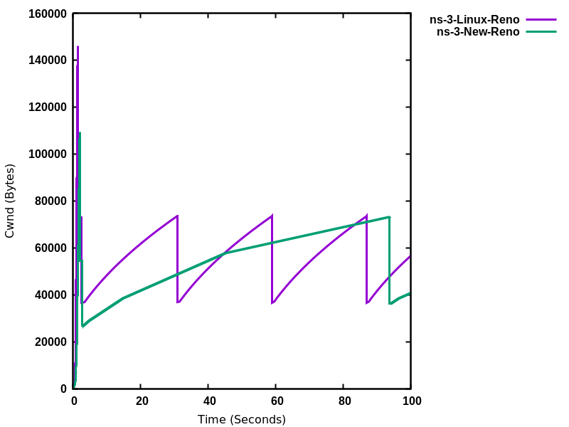
ns-3 TCP NewReno vs. ns-3 TCP Linux Reno
HighSpeed
TCP HighSpeed is designed for high-capacity channels or, in general, for TCP connections with large congestion windows. Conceptually, with respect to the standard TCP, HighSpeed makes the cWnd grow faster during the probing phases and accelerates the cWnd recovery from losses. This behavior is executed only when the window grows beyond a certain threshold, which allows TCP HighSpeed to be friendly with standard TCP in environments with heavy congestion, without introducing new dangers of congestion collapse.
Mathematically:
(4)
The function a() is calculated using a fixed RTT the value 100 ms (the lookup table for this function is taken from RFC 3649). For each congestion event, the slow start threshold is decreased by a value that depends on the size of the slow start threshold itself. Then, the congestion window is set to such value.
(5)
The lookup table for the function b() is taken from the same RFC. More information at: http://dl.acm.org/citation.cfm?id=2756518
Hybla
The key idea behind TCP Hybla is to obtain for long RTT connections the same instantaneous transmission rate of a reference TCP connection with lower RTT. With analytical steps, it is shown that this goal can be achieved by modifying the time scale, in order for the throughput to be independent from the RTT. This independence is obtained through the use of a coefficient rho.
This coefficient is used to calculate both the slow start threshold and the congestion window when in slow start and in congestion avoidance, respectively.
More information at: http://dl.acm.org/citation.cfm?id=2756518
Westwood
Westwood and Westwood+ employ the AIAD (Additive Increase/Adaptive Decrease)· congestion control paradigm. When a congestion episode happens,· instead of halving the cwnd, these protocols try to estimate the network’s bandwidth and use the estimated value to adjust the cwnd.· While Westwood performs the bandwidth sampling every ACK reception,· Westwood+ samples the bandwidth every RTT.
More information at: http://dl.acm.org/citation.cfm?id=381704 and http://dl.acm.org/citation.cfm?id=2512757
Vegas
TCP Vegas is a pure delay-based congestion control algorithm implementing a proactive scheme that tries to prevent packet drops by maintaining a small backlog at the bottleneck queue. Vegas continuously samples the RTT and computes the actual throughput a connection achieves using Equation (6) and compares it with the expected throughput calculated in Equation (7). The difference between these 2 sending rates in Equation (8) reflects the amount of extra packets being queued at the bottleneck.
(6)
(7)
(8)
To avoid congestion, Vegas linearly increases/decreases its congestion window to ensure the diff value falls between the two predefined thresholds, alpha and beta. diff and another threshold, gamma, are used to determine when Vegas should change from its slow-start mode to linear increase/decrease mode. Following the implementation of Vegas in Linux, we use 2, 4, and 1 as the default values of alpha, beta, and gamma, respectively, but they can be modified through the Attribute system.
More information at: http://dx.doi.org/10.1109/49.464716
Scalable
Scalable improves TCP performance to better utilize the available bandwidth of a highspeed wide area network by altering NewReno congestion window adjustment algorithm. When congestion has not been detected, for each ACK received in an RTT, Scalable increases its cwnd per:
(9)
Following Linux implementation of Scalable, we use 50 instead of 100 to account for delayed ACK.
On the first detection of congestion in a given RTT, cwnd is reduced based on the following equation:
(10)
More information at: http://dl.acm.org/citation.cfm?id=956989
Veno
TCP Veno enhances Reno algorithm for more effectively dealing with random packet loss in wireless access networks by employing Vegas’s method in estimating the backlog at the bottleneck queue to distinguish between congestive and non-congestive states.
The backlog (the number of packets accumulated at the bottleneck queue) is calculated using Equation (11):
(11)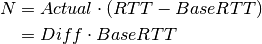
where:
(12)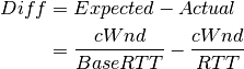
Veno makes decision on cwnd modification based on the calculated N and its predefined threshold beta.
Specifically, it refines the additive increase algorithm of Reno so that the connection can stay longer in the stable state by incrementing cwnd by 1/cwnd for every other new ACK received after the available bandwidth has been fully utilized, i.e. when N exceeds beta. Otherwise, Veno increases its cwnd by 1/cwnd upon every new ACK receipt as in Reno.
In the multiplicative decrease algorithm, when Veno is in the non-congestive state, i.e. when N is less than beta, Veno decrements its cwnd by only 1/5 because the loss encountered is more likely a corruption-based loss than a congestion-based. Only when N is greater than beta, Veno halves its sending rate as in Reno.
More information at: http://dx.doi.org/10.1109/JSAC.2002.807336
BIC
BIC (class TcpBic) is a predecessor of TCP CUBIC.
In TCP BIC the congestion control problem is viewed as a search
problem. Taking as a starting point the current window value
and as a target point the last maximum window value
(i.e. the cWnd value just before the loss event) a binary search
technique can be used to update the cWnd value at the midpoint between
the two, directly or using an additive increase strategy if the distance from
the current window is too large.
This way, assuming a no-loss period, the congestion window logarithmically approaches the maximum value of cWnd until the difference between it and cWnd falls below a preset threshold. After reaching such a value (or the maximum window is unknown, i.e. the binary search does not start at all) the algorithm switches to probing the new maximum window with a ‘slow start’ strategy.
If a loss occur in either these phases, the current window (before the loss) can be treated as the new maximum, and the reduced (with a multiplicative decrease factor Beta) window size can be used as the new minimum.
More information at: http://ieeexplore.ieee.org/xpl/articleDetails.jsp?arnumber=1354672
YeAH
YeAH-TCP (Yet Another HighSpeed TCP) is a heuristic designed to balance various requirements of a state-of-the-art congestion control algorithm:
- fully exploit the link capacity of high BDP networks while inducing a small number of congestion events
- compete friendly with Reno flows
- achieve intra and RTT fairness
- robust to random losses
- achieve high performance regardless of buffer size
YeAH operates between 2 modes: Fast and Slow mode. In the Fast mode when the queue occupancy is small and the network congestion level is low, YeAH increments its congestion window according to the aggressive HSTCP rule. When the number of packets in the queue grows beyond a threshold and the network congestion level is high, YeAH enters its Slow mode, acting as Reno with a decongestion algorithm. YeAH employs Vegas’ mechanism for calculating the backlog as in Equation (13). The estimation of the network congestion level is shown in Equation (14).
(13)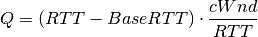
(14)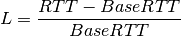
To ensure TCP friendliness, YeAH also implements an algorithm to detect the presence of legacy Reno flows. Upon the receipt of 3 duplicate ACKs, YeAH decreases its slow start threshold according to Equation (15) if it’s not competing with Reno flows. Otherwise, the ssthresh is halved as in Reno:
(15)
More information: http://www.csc.lsu.edu/~sjpark/cs7601/4-YeAH_TCP.pdf
Illinois
TCP Illinois is a hybrid congestion control algorithm designed for high-speed networks. Illinois implements a Concave-AIMD (or C-AIMD) algorithm that uses packet loss as the primary congestion signal to determine the direction of window update and queueing delay as the secondary congestion signal to determine the amount of change.
The additive increase and multiplicative decrease factors (denoted as alpha and beta, respectively) are functions of the current average queueing delay da as shown in Equations (16) and (17). To improve the protocol robustness against sudden fluctuations in its delay sampling, Illinois allows the increment of alpha to alphaMax only if da stays below d1 for a some (theta) amount of time.
(16)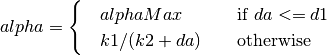
(17)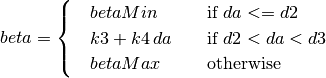
where the calculations of k1, k2, k3, and k4 are shown in the following:
(18)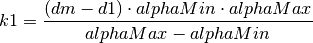
(19)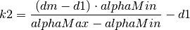
(20)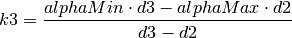
(21)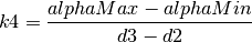
Other parameters include da (the current average queueing delay), and Ta (the average RTT, calculated as sumRtt / cntRtt in the implementation) and Tmin (baseRtt in the implementation) which is the minimum RTT ever seen. dm is the maximum (average) queueing delay, and Tmax (maxRtt in the implementation) is the maximum RTT ever seen.
(22)
(23)
(24)
Illinois only executes its adaptation of alpha and beta when cwnd exceeds a threshold called winThresh. Otherwise, it sets alpha and beta to the base values of 1 and 0.5, respectively.
Following the implementation of Illinois in the Linux kernel, we use the following default parameter settings:
- alphaMin = 0.3 (0.1 in the Illinois paper)
- alphaMax = 10.0
- betaMin = 0.125
- betaMax = 0.5
- winThresh = 15 (10 in the Illinois paper)
- theta = 5
- eta1 = 0.01
- eta2 = 0.1
- eta3 = 0.8
More information: http://www.doi.org/10.1145/1190095.1190166
H-TCP
H-TCP has been designed for high BDP (Bandwidth-Delay Product) paths. It is
a dual mode protocol. In normal conditions, it works like traditional TCP
with the same rate of increment and decrement for the congestion window.
However, in high BDP networks, when it finds no congestion on the path
after deltal seconds, it increases the window size based on the alpha
function in the following:
(25)
where deltal is a threshold in seconds for switching between the modes and
delta is the elapsed time from the last congestion. During congestion,
it reduces the window size by multiplying by beta function provided
in the reference paper. The calculated throughput between the last two
consecutive congestion events is considered for beta calculation.
The transport TcpHtcp can be selected in the program
examples/tcp/tcp-variants-comparison.cc to perform an experiment with H-TCP,
although it is useful to increase the bandwidth in this example (e.g.
to 20 Mb/s) to create a higher BDP link, such as
./waf --run "tcp-variants-comparison --transport_prot=TcpHtcp --bandwidth=20Mbps --duration=10"
More information (paper): http://www.hamilton.ie/net/htcp3.pdf
More information (Internet Draft): https://tools.ietf.org/html/draft-leith-tcp-htcp-06
LEDBAT
Low Extra Delay Background Transport (LEDBAT) is an experimental delay-based congestion control algorithm that seeks to utilize the available bandwidth on an end-to-end path while limiting the consequent increase in queueing delay on that path. LEDBAT uses changes in one-way delay measurements to limit congestion that the flow itself induces in the network.
As a first approximation, the LEDBAT sender operates as shown below:
On receipt of an ACK:
- ::
- currentdelay = acknowledgement.delay basedelay = min (basedelay, currentdelay) queuingdelay = currentdelay - basedelay offtarget = (TARGET - queuingdelay) / TARGET cWnd += GAIN * offtarget * bytesnewlyacked * MSS / cWnd
TARGET is the maximum queueing delay that LEDBAT itself may introduce in the
network, and GAIN determines the rate at which the cwnd responds to changes in
queueing delay; offtarget is a normalized value representing the difference between
the measured current queueing delay and the predetermined TARGET delay. offtarget can
be positive or negative; consequently, cwnd increases or decreases in proportion to
offtarget.
Following the recommendation of RFC 6817, the default values of the parameters are:
- TargetDelay = 100
- baseHistoryLen = 10
- noiseFilterLen = 4
- Gain = 1
To enable LEDBAT on all TCP sockets, the following configuration can be used:
Config::SetDefault ("ns3::TcpL4Protocol::SocketType", TypeIdValue (TcpLedbat::GetTypeId ()));
To enable LEDBAT on a chosen TCP socket, the following configuration can be used:
Config::Set ("$ns3::NodeListPriv/NodeList/1/$ns3::TcpL4Protocol/SocketType", TypeIdValue (TcpLedbat::GetTypeId ()));
The following unit tests have been written to validate the implementation of LEDBAT:
- LEDBAT should operate same as NewReno during slow start
- LEDBAT should operate same as NewReno if timestamps are disabled
- Test to validate cwnd increment in LEDBAT
In comparison to RFC 6817, the scope and limitations of the current LEDBAT implementation are:
- It assumes that the clocks on the sender side and receiver side are synchronised
- In line with Linux implementation, the one-way delay is calculated at the sender side by using the timestamps option in TCP header
- Only the MIN function is used for noise filtering
More information about LEDBAT is available in RFC 6817: https://tools.ietf.org/html/rfc6817
TCP-LP
TCP-Low Priority (TCP-LP) is a delay based congestion control protocol in which the low priority data utilizes only the excess bandwidth available on an end-to-end path. TCP-LP uses one way delay measurements as an indicator of congestion as it does not influence cross-traffic in the reverse direction.
On receipt of an ACK:

where owdMin and owdMax are the minimum and maximum one way delays experienced throughout the connection, LP_WITHIN_INF indicates if TCP-LP is in inference phase or not
More information (paper): http://cs.northwestern.edu/~akuzma/rice/doc/TCP-LP.pdf
Data Center TCP (DCTCP)
DCTCP, specified in RFC 8257 and implemented in Linux, is a TCP congestion control algorithm for data center networks. It leverages Explicit Congestion Notification (ECN) to provide more fine-grained congestion feedback to the end hosts, and is intended to work with routers that implement a shallow congestion marking threshold (on the order of a few milliseconds) to achieve high throughput and low latency in the datacenter. However, because DCTCP does not react in the same way to notification of congestion experienced, there are coexistence (fairness) issues between it and legacy TCP congestion controllers, which is why it is recommended to only be used in controlled networking environments such as within data centers.
DCTCP extends the Explicit Congestion Notification signal to estimate the fraction of bytes that encounter congestion, rather than simply detecting that the congestion has occurred. DCTCP then scales the congestion window based on this estimate. This approach achieves high burst tolerance, low latency, and high throughput with shallow-buffered switches.
- Receiver functionality: If CE is observed in the IP header of an incoming packet at the TCP receiver, the receiver sends congestion notification to the sender by setting ECE in TCP header. This processing is different from standard receiver ECN processing which sets and holds the ECE bit for every ACK until it observes a CWR signal from the TCP sender.
- Sender functionality: The sender makes use of the modified receiver
ECE semantics to maintain an estimate of the fraction of packets marked
(
 ) by using the exponential weighted moving average (EWMA) as
shown below:
) by using the exponential weighted moving average (EWMA) as
shown below:

In the above EWMA:
- g is the estimation gain (between 0 and 1)
- F is the fraction of packets marked in current RTT.
For send windows in which at least one ACK was received with ECE set, the sender should respond by reducing the congestion window as follows, once for every window of data:

Following the recommendation of RFC 8257, the default values of the parameters are:
To enable DCTCP on all TCP sockets, the following configuration can be used:
Config::SetDefault ("ns3::TcpL4Protocol::SocketType", TypeIdValue (TcpDctcp::GetTypeId ()));
To enable DCTCP on a selected node, one can set the “SocketType” attribute on the TcpL4Protocol object of that node to the TcpDctcp TypeId.
The ECN is enabled automatically when DCTCP is used, even if the user has not explicitly enabled it.
DCTCP depends on a simple queue management algorithm in routers / switches to mark packets. The current implementation of DCTCP in ns-3 can use RED with a simple configuration to achieve the behavior of desired queue management algorithm.
To configure RED router for DCTCP:
Config::SetDefault ("ns3::RedQueueDisc::UseEcn", BooleanValue (true));
Config::SetDefault ("ns3::RedQueueDisc::QW", DoubleValue (1.0));
Config::SetDefault ("ns3::RedQueueDisc::MinTh", DoubleValue (16));
Config::SetDefault ("ns3::RedQueueDisc::MaxTh", DoubleValue (16));
There is also the option, when running CoDel or FqCoDel, to enable ECN on the queue and to set the “CeThreshold” value to a low value such as 1ms. The following example uses CoDel:
Config::SetDefault ("ns3::CoDelQueueDisc::UseEcn", BooleanValue (true));
Config::SetDefault ("ns3::CoDelQueueDisc::CeThreshold", TimeValue (MilliSeconds (1)));
The following unit tests have been written to validate the implementation of DCTCP:
- ECT flags should be set for SYN, SYN+ACK, ACK and data packets for DCTCP traffic
- ECT flags should not be set for SYN, SYN+ACK and pure ACK packets, but should be set on data packets for ECN enabled traditional TCP flows
- ECE should be set only when CE flags are received at receiver and even if sender doesn’t send CWR, receiver should not send ECE if it doesn’t receive packets with CE flags
An example program, examples/tcp/tcp-validation.cc, can be used to
experiment with DCTCP for long-running flows with different bottleneck
link bandwidth, base RTTs, and queuing disciplines. A variant of this
program has also been run using the ns-3 Direct Code Execution
environment using DCTCP from Linux kernel 4.4, and the results were
compared against ns-3 results.
An example program based on an experimental topology found in the original
DCTCP SIGCOMM paper is provided in examples/tcp/dctcp-example.cc.
This example uses a simple topology consisting of forty DCTCP senders
and receivers and two ECN-enabled switches to examine throughput,
fairness, and queue delay properties of the network.
This implementation was tested extensively against a version of DCTCP in the Linux kernel version 4.4 using the ns-3 direct code execution (DCE) environment. Some differences were noted:
- Linux maintains its congestion window in segments and not bytes, and the arithmetic is not floating point, so small differences in the evolution of congestion window have been observed.
- Linux uses pacing, where packets to be sent are paced out at regular intervals. However, if at any instant the number of segments that can be sent are less than two, Linux does not pace them and instead sends them back-to-back. Currently, ns-3 paces out all packets eligible to be sent in the same manner.
More information about DCTCP is available in the RFC 8257: https://tools.ietf.org/html/rfc8257
BBR
BBR (class TcpBbr) is a congestion control algorithm that
regulates the sending rate by deriving an estimate of the bottleneck’s
available bandwidth and RTT of the path. It seeks to operate at an optimal
point where sender experiences maximum delivery rate with minimum RTT. It
creates a network model comprising maximum delivery rate with minimum RTT
observed so far, and then estimates BDP (maximum bandwidth * minimum RTT)
to control the maximum amount of inflight data. BBR controls congestion by
limiting the rate at which packets are sent. It caps the cwnd to one BDP
and paces out packets at a rate which is adjusted based on the latest estimate
of delivery rate. BBR algorithm is agnostic to packet losses and ECN marks.
pacing_gain controls the rate of sending data and cwnd_gain controls the amount of data to send.
The following is a high level overview of BBR congestion control algorithm:
- On receiving an ACK:
- rtt = now - packet.sent_time update_minimum_rtt (rtt) delivery_rate = estimate_delivery_rate (packet) update_maximum_bandwidth (delivery_rate)
- After transmitting a data packet:
bdp = max_bandwidth * min_rtt if (cwnd * bdp < inflight)
return- if (now > nextSendTime)
- {
- transmit (packet) nextSendTime = now + packet.size / (pacing_gain * max_bandwidth)
}
- else
- return
Schedule (nextSendTime, Send)
To enable BBR on all TCP sockets, the following configuration can be used:
Config::SetDefault ("ns3::TcpL4Protocol::SocketType", TypeIdValue (TcpBbr::GetTypeId ()));
To enable BBR on a chosen TCP socket, the following configuration can be used (note that an appropriate Node ID must be used instead of 1):
Config::Set ("$ns3::NodeListPriv/NodeList/1/$ns3::TcpL4Protocol/SocketType", TypeIdValue (TcpBbr::GetTypeId ()));
The ns-3 implementation of BBR is based on its Linux implementation. Linux 5.4 kernel implementation has been used to validate the behavior of ns-3 implementation of BBR (See below section on Validation).
In addition, the following unit tests have been written to validate the implementation of BBR in ns-3:
- BBR should enable (if not already done) TCP pacing feature.
- Test to validate the values of pacing_gain and cwnd_gain in different phases
of BBR.
An example program, examples/tcp/tcp-bbr-example.cc, is provided to experiment with BBR for one long running flow. This example uses a simple topology consisting of one sender, one receiver and two routers to examine congestion window, throughput and queue control. A program similar to this has been run using the Network Stack Tester (NeST) using BBR from Linux kernel 5.4, and the results were compared against ns-3 results.
More information about BBR is available in the following Internet Draft: https://tools.ietf.org/html/draft-cardwell-iccrg-bbr-congestion-control-00
More information about Delivery Rate Estimation is in the following draft: https://tools.ietf.org/html/draft-cheng-iccrg-delivery-rate-estimation-00
For an academic peer-reviewed paper on the BBR implementation in ns-3, please refer to:
- Vivek Jain, Viyom Mittal and Mohit P. Tahiliani. “Design and Implementation of TCP BBR in ns-3.” In Proceedings of the 10th Workshop on ns-3, pp. 16-22. 2018. (https://dl.acm.org/doi/abs/10.1145/3199902.3199911)
Support for Explicit Congestion Notification (ECN)
ECN provides end-to-end notification of network congestion without dropping packets. It uses two bits in the IP header: ECN Capable Transport (ECT bit) and Congestion Experienced (CE bit), and two bits in the TCP header: Congestion Window Reduced (CWR) and ECN Echo (ECE).
More information is available in RFC 3168: https://tools.ietf.org/html/rfc3168
The following ECN states are declared in src/internet/model/tcp-socket-state.h
typedef enum
  {
    ECN_DISABLED = 0, //!< ECN disabled traffic
    ECN_IDLE,         //!< ECN is enabled but currently there is no action pertaining to ECE or CWR to be taken
    ECN_CE_RCVD,      //!< Last packet received had CE bit set in IP header
    ECN_SENDING_ECE,  //!< Receiver sends an ACK with ECE bit set in TCP header
    ECN_ECE_RCVD,     //!< Last ACK received had ECE bit set in TCP header
    ECN_CWR_SENT      //!< Sender has reduced the congestion window, and sent a packet with CWR bit set in TCP header. This is used for tracing.
  } EcnStates_t;
Current implementation of ECN is based on RFC 3168 and is referred as Classic ECN.
The following enum represents the mode of ECN:
typedef enum
  {
    ClassicEcn,  //!< ECN functionality as described in RFC 3168.
    DctcpEcn,    //!< ECN functionality as described in RFC 8257. Note: this mode is specific to DCTCP.
  } EcnMode_t;
The following are some important ECN parameters:
// ECN parameters
EcnMode_t              m_ecnMode {ClassicEcn}; //!< ECN mode
UseEcn_t               m_useEcn {Off};         //!< Socket ECN capability
Enabling ECN
By default, support for ECN is disabled in TCP sockets. To enable, change
the value of the attribute ns3::TcpSocketBase::UseEcn to On.
Following are supported values for the same, this functionality is aligned with
Linux: https://www.kernel.org/doc/Documentation/networking/ip-sysctl.txt
typedef enum
  {
    Off        = 0,   //!< Disable
    On         = 1,   //!< Enable
    AcceptOnly = 2,   //!< Enable only when the peer endpoint is ECN capable
  } UseEcn_t;
For example:
Config::SetDefault ("ns3::TcpSocketBase::UseEcn", StringValue ("On"))
ECN negotiation
ECN capability is negotiated during the three-way TCP handshake:
- Sender sends SYN + CWR + ECE
if (m_useEcn == UseEcn_t::On)
  {
    SendEmptyPacket (TcpHeader::SYN | TcpHeader::ECE | TcpHeader::CWR);
  }
else
  {
    SendEmptyPacket (TcpHeader::SYN);
  }
m_ecnState = ECN_DISABLED;
- Receiver sends SYN + ACK + ECE
if (m_useEcn != UseEcn_t::Off && (tcpHeader.GetFlags () & (TcpHeader::CWR | TcpHeader::ECE)) == (TcpHeader::CWR | TcpHeader::ECE))
  {
    SendEmptyPacket (TcpHeader::SYN | TcpHeader::ACK |TcpHeader::ECE);
    m_ecnState = ECN_IDLE;
  }
else
  {
    SendEmptyPacket (TcpHeader::SYN | TcpHeader::ACK);
    m_ecnState = ECN_DISABLED;
  }
- Sender sends ACK
if (m_useEcn != UseEcn_t::Off &&  (tcpHeader.GetFlags () & (TcpHeader::CWR | TcpHeader::ECE)) == (TcpHeader::ECE))
  {
    m_ecnState = ECN_IDLE;
  }
else
  {
    m_ecnState = ECN_DISABLED;
  }
Once the ECN-negotiation is successful, the sender sends data packets with ECT bits set in the IP header.
Note: As mentioned in Section 6.1.1 of RFC 3168, ECT bits should not be set during ECN negotiation. The ECN negotiation implemented in ns-3 follows this guideline.
ECN State Transitions
- Initially both sender and receiver have their m_ecnState set as ECN_DISABLED
- Once the ECN negotiation is successful, their states are set to ECN_IDLE
- The receiver’s state changes to ECN_CE_RCVD when it receives a packet with CE bit set. The state then moves to ECN_SENDING_ECE when the receiver sends an ACK with ECE set. This state is retained until a CWR is received , following which, the state changes to ECN_IDLE.
- When the sender receives an ACK with ECE bit set from receiver, its state is set as ECN_ECE_RCVD
- The sender’s state changes to ECN_CWR_SENT when it sends a packet with CWR bit set. It remains in this state until an ACK with valid ECE is received (i.e., ECE is received for a packet that belongs to a new window), following which, its state changes to ECN_ECE_RCVD.
RFC 3168 compliance
Based on the suggestions provided in RFC 3168, the following behavior has been implemented:
- Pure ACK packets should not have the ECT bit set (Section 6.1.4).
- In the current implementation, the sender only sends ECT(0) in the IP header.
- The sender should should reduce the congestion window only once in each window (Section 6.1.2).
- The receiver should ignore the CE bits set in a packet arriving out of window (Section 6.1.5).
- The sender should ignore the ECE bits set in the packet arriving out of window (Section 6.1.2).
Open issues
The following issues are yet to be addressed:
- Retransmitted packets should not have the CWR bit set (Section 6.1.5).
- Despite the congestion window size being 1 MSS, the sender should reduce its congestion window by half when it receives a packet with the ECE bit set. The sender must reset the retransmit timer on receiving the ECN-Echo packet when the congestion window is one. The sending TCP will then be able to send a new packet only when the retransmit timer expires (Section 6.1.2).
- Support for separately handling the enabling of ECN on the incoming and outgoing TCP sessions (e.g. a TCP may perform ECN echoing but not set the ECT codepoints on its outbound data segments).
Support for Dynamic Pacing
TCP pacing refers to the sender-side practice of scheduling the transmission of a burst of eligible TCP segments across a time interval such as a TCP RTT, to avoid or reduce bursts. Historically, TCP used the natural ACK clocking mechanism to pace segments, but some network paths introduce aggregation (bursts of ACKs arriving) or ACK thinning, either of which disrupts ACK clocking. Some latency-sensitive congestion controls under development (Prague, BBR) require pacing to operate effectively.
Until recently, the state of the art in Linux was to support pacing in one of two ways:
- fq/pacing with sch_fq
- TCP internal pacing
The presentation by Dumazet and Cheng at IETF 88 summarizes: https://www.ietf.org/proceedings/88/slides/slides-88-tcpm-9.pdf
The first option was most often used when offloading (TSO) was enabled and when the sch_fq scheduler was used at the traffic control (qdisc) sublayer. In this case, TCP was responsible for setting the socket pacing rate, but the qdisc sublayer would enforce it. When TSO was enabled, the kernel would break a large burst into smaller chunks, with dynamic sizing based on the pacing rate, and hand off the segments to the fq qdisc for pacing.
The second option was used if sch_fq was not enabled; TCP would be responsible for internally pacing.
In 2018, Linux switched to an Early Departure Model (EDM): https://lwn.net/Articles/766564/.
TCP pacing in Linux was added in kernel 3.12, and authors chose to allow a pacing rate of 200% against the current rate, to allow probing for optimal throughput even during slow start phase. Some refinements were added in https://git.kernel.org/pub/scm/linux/kernel/git/torvalds/linux.git/commit/?id=43e122b014c9, in which Google reported that it was better to apply a different ratio (120%) in Congestion Avoidance phase. Furthermore, authors found that after cwnd reduction, it was helpful to become more conservative and switch to the conservative ratio (120%) as soon as cwnd >= ssthresh/2, as the initial ramp up (when ssthresh is infinite) still allows doubling cwnd every other RTT. Linux also does not pace the initial window (IW), typically 10 segments in practice.
Linux has also been observed to not pace if the number of eligible segments to be sent is exactly two; they will be sent back to back. If three or more, the first two are sent immediately, and additional segments are paced at the current pacing rate.
In ns-3, the model is as follows. There is no TSO/sch_fq model; only internal pacing according to current Linux policy.
Pacing may be enabled for any TCP congestion control, and a maximum pacing rate can be set. Furthermore, dynamic pacing is enabled for all TCP variants, according to the following guidelines.
- Pacing of the initial window (IW) is not done by default but can be separately enabled.
- Pacing of the initial slow start, after IW, is done according to the pacing rate of 200% of the current rate, to allow for window growth This pacing rate can be configured to a different value than 200%.
- Pacing of congestion avoidance phase is done at a pacing rate of 120% of current rate. This can be configured to a different value than 120%.
- Pacing of subsequent slow start is done according to the following heuristic. If cwnd < ssthresh/2, such as after a timeout or idle period, pace at the slow start rate (200%). Otherwise, pace at the congestion avoidance rate.
Dynamic pacing is demonstrated by the example program examples/tcp/tcp-pacing.cc.
Validation
The following tests are found in the src/internet/test directory. In
general, TCP tests inherit from a class called TcpGeneralTest,
which provides common operations to set up test scenarios involving TCP
objects. For more information on how to write new tests, see the
section below on Writing TCP tests.
- tcp: Basic transmission of string of data from client to server
- tcp-bytes-in-flight-test: TCP correctly estimates bytes in flight under loss conditions
- tcp-cong-avoid-test: TCP congestion avoidance for different packet sizes
- tcp-datasentcb: Check TCP’s ‘data sent’ callback
- tcp-endpoint-bug2211-test: A test for an issue that was causing stack overflow
- tcp-fast-retr-test: Fast Retransmit testing
- tcp-header: Unit tests on the TCP header
- tcp-highspeed-test: Unit tests on the HighSpeed congestion control
- tcp-htcp-test: Unit tests on the H-TCP congestion control
- tcp-hybla-test: Unit tests on the Hybla congestion control
- tcp-vegas-test: Unit tests on the Vegas congestion control
- tcp-veno-test: Unit tests on the Veno congestion control
- tcp-scalable-test: Unit tests on the Scalable congestion control
- tcp-bic-test: Unit tests on the BIC congestion control
- tcp-yeah-test: Unit tests on the YeAH congestion control
- tcp-illinois-test: Unit tests on the Illinois congestion control
- tcp-ledbat-test: Unit tests on the LEDBAT congestion control
- tcp-lp-test: Unit tests on the TCP-LP congestion control
- tcp-dctcp-test: Unit tests on the DCTCP congestion control
- tcp-bbr-test: Unit tests on the BBR congestion control
- tcp-option: Unit tests on TCP options
- tcp-pkts-acked-test: Unit test the number of time that PktsAcked is called
- tcp-rto-test: Unit test behavior after a RTO occurs
- tcp-rtt-estimation-test: Check RTT calculations, including retransmission cases
- tcp-slow-start-test: Check behavior of slow start
- tcp-timestamp: Unit test on the timestamp option
- tcp-wscaling: Unit test on the window scaling option
- tcp-zero-window-test: Unit test persist behavior for zero window conditions
- tcp-close-test: Unit test on the socket closing: both receiver and sender have to close their socket when all bytes are transferred
- tcp-ecn-test: Unit tests on Explicit Congestion Notification
- tcp-pacing-test: Unit tests on dynamic TCP pacing rate
Several tests have dependencies outside of the internet module, so they
are located in a system test directory called src/test/ns3tcp. Three
of these six tests involve use of the Network Simulation Cradle, and are
disabled if NSC is not enabled in the build.
- ns3-tcp-cwnd: Check to see that ns-3 TCP congestion control works against liblinux2.6.26.so implementation
- ns3-tcp-interoperability: Check to see that ns-3 TCP interoperates with liblinux2.6.26.so implementation
- ns3-tcp-loss: Check behavior of ns-3 TCP upon packet losses
- nsc-tcp-loss: Check behavior of NSC TCP upon packet losses
- ns3-tcp-no-delay: Check that ns-3 TCP Nagle’s algorithm works correctly and that it can be disabled
- ns3-tcp-socket: Check that ns-3 TCP successfully transfers an application data write of various sizes
- ns3-tcp-state: Check the operation of the TCP state machine for several cases
Several TCP validation test results can also be found in the wiki page describing this implementation.
The ns-3 implementation of TCP Linux Reno was validated against the NewReno implementation of Linux kernel 4.4.0 using ns-3 Direct Code Execution (DCE). DCE is a framework which allows the users to run kernel space protocol inside ns-3 without changing the source code.
In this validation, cwnd traces of DCE Linux reno were compared to those of
ns-3 Linux Reno and NewReno for a delayed acknowledgement configuration of 1
segment (in the ns-3 implementation; Linux does not allow direct configuration
of this setting). It can be observed that cwnd traces for ns-3 Linux Reno are
closely overlapping with DCE reno, while
for ns-3 NewReno there was deviation in the congestion avoidance phase.
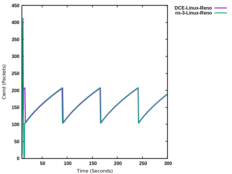
DCE Linux Reno vs. ns-3 Linux Reno
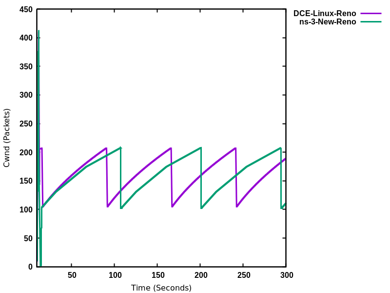
DCE Linux Reno vs. ns-3 NewReno
The difference in the cwnd in the early stage of this flow is because of the way cwnd is plotted. As ns-3 provides a trace source for cwnd, an ns-3 Linux Reno cwnd simple is obtained every time the cwnd value changes, whereas for DCE Linux Reno, the kernel does not have a corresponding trace source. Instead, we use the “ss” command of the Linux kernel to obtain cwnd values. The “ss” samples cwnd at an interval of 0.5 seconds.
Figure DCTCP throughput for 10ms/50Mbps bottleneck, 1ms CE threshold shows a long-running file transfer using DCTCP over a 50 Mbps bottleneck (running CoDel queue disc with a 1ms CE threshold setting) with a 10 ms base RTT. The figure shows that DCTCP reaches link capacity very quickly and stays there for the duration with minimal change in throughput. In contrast, Figure DCTCP throughput for 80ms/50Mbps bottleneck, 1ms CE threshold plots the throughput for the same configuration except with an 80 ms base RTT. In this case, the DCTCP exits slow start early and takes a long time to build the flow throughput to the bottleneck link capacity. DCTCP is not intended to be used at such a large base RTT, but this figure highlights the sensitivity to RTT (and can be reproduced using the Linux implementation).
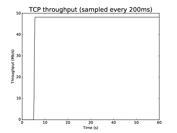
DCTCP throughput for 10ms/50Mbps bottleneck, 1ms CE threshold
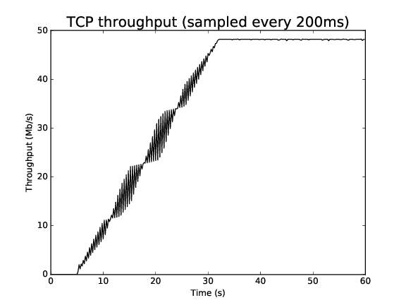
DCTCP throughput for 80ms/50Mbps bottleneck, 1ms CE threshold
Similar to DCTCP, TCP CUBIC has been tested against the Linux kernel version 4.4 implementation. Figure CUBIC cwnd evolution for 50ms/50Mbps bottleneck, no ECN compares the congestion window evolution between ns-3 and Linux for a single flow operating over a 50 Mbps link with 50 ms base RTT and the CoDel AQM. Some differences can be observed between the peak of slow start window growth (ns-3 exits slow start earlier due to its HyStart implementation), and the window growth is a bit out-of-sync (likely due to different implementations of the algorithm), but the cubic concave/convex window pattern, and the signs of TCP CUBIC fast convergence algorithm (alternating patterns of cubic and concave window growth) can be observed. The ns-3 congestion window is maintained in bytes (unlike Linux which uses segments) but has been normalized to segments for these plots. Figure CUBIC cwnd evolution for 50ms/50Mbps bottleneck, with ECN displays the outcome of a similar scenario but with ECN enabled throughout.
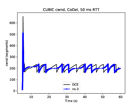
CUBIC cwnd evolution for 50ms/50Mbps bottleneck, no ECN

CUBIC cwnd evolution for 50ms/50Mbps bottleneck, with ECN
TCP ECN operation is tested in the ARED and RED tests that are documented in the traffic-control module documentation.
Like DCTCP and TCP CUBIC, the ns-3 implementation of TCP BBR was validated against the BBR implementation of Linux kernel 5.4 using Network Stack Tester (NeST). NeST is a python package which allows the users to emulate kernel space protocols using Linux network namespaces. Figure Congestion window evolution: ns-3 BBR vs. Linux BBR (using NeST) compares the congestion window evolution between ns-3 and Linux for a single flow operating over a 10 Mbps link with 10 ms base RTT and FIFO queue discipline.
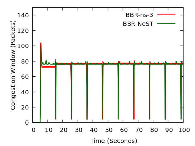
Congestion window evolution: ns-3 BBR vs. Linux BBR (using NeST)
It can be observed that the congestion window traces for ns-3 BBR closely overlap with Linux BBR. The periodic drops in congestion window every 10 seconds depict the PROBE_RTT phase of the BBR algorithm. In this phase, BBR algorithm keeps the congestion window fixed to 4 segments.
The example program, examples/tcp-bbr-example.cc has been used to obtain the congestion window curve shown in Figure Congestion window evolution: ns-3 BBR vs. Linux BBR (using NeST). The detailed instructions to reproduce ns-3 plot and NeST plot can be found at: https://github.com/mohittahiliani/BBR-Validation
Writing a new congestion control algorithm
Writing (or porting) a congestion control algorithms from scratch (or from other systems) is a process completely separated from the internals of TcpSocketBase.
All operations that are delegated to a congestion control are contained in the class TcpCongestionOps. It mimics the structure tcp_congestion_ops of Linux, and the following operations are defined:
virtual std::string GetName () const;
virtual uint32_t GetSsThresh (Ptr<const TcpSocketState> tcb, uint32_t bytesInFlight);
virtual void IncreaseWindow (Ptr<TcpSocketState> tcb, uint32_t segmentsAcked);
virtual void PktsAcked (Ptr<TcpSocketState> tcb, uint32_t segmentsAcked,const Time& rtt);
virtual Ptr<TcpCongestionOps> Fork ();
virtual void CwndEvent (Ptr<TcpSocketState> tcb, const TcpSocketState::TcpCaEvent_t event);
The most interesting methods to write are GetSsThresh and IncreaseWindow. The latter is called when TcpSocketBase decides that it is time to increase the congestion window. Much information is available in the Transmission Control Block, and the method should increase cWnd and/or ssThresh based on the number of segments acked.
GetSsThresh is called whenever the socket needs an updated value of the slow start threshold. This happens after a loss; congestion control algorithms are then asked to lower such value, and to return it.
PktsAcked is used in case the algorithm needs timing information (such as RTT), and it is called each time an ACK is received.
CwndEvent is used in case the algorithm needs the state of socket during different congestion window event.
TCP SACK and non-SACK
To avoid code duplication and the effort of maintaining two different versions of the TCP core, namely RFC 6675 (TCP-SACK) and RFC 5681 (TCP congestion control), we have merged RFC 6675 in the current code base. If the receiver supports the option, the sender bases its retransmissions over the received SACK information. However, in the absence of that option, the best it can do is to follow the RFC 5681 specification (on Fast Retransmit/Recovery) and employing NewReno modifications in case of partial ACKs.
A similar concept is used in Linux with the function tcp_add_reno_sack. Our implementation resides in the TcpTxBuffer class that implements a scoreboard through two different lists of segments. TcpSocketBase actively uses the API provided by TcpTxBuffer to query the scoreboard; please refer to the Doxygen documentation (and to in-code comments) if you want to learn more about this implementation.
For an academic peer-reviewed paper on the SACK implementation in ns-3, please refer to https://dl.acm.org/citation.cfm?id=3067666.
Loss Recovery Algorithms
The following loss recovery algorithms are supported in ns-3 TCP. The current default (as of ns-3.32 release) is Proportional Rate Reduction (PRR), while the default for ns-3.31 and earlier was Classic Recovery.
Classic Recovery
Classic Recovery refers to the combination of NewReno algorithm described in RFC 6582 along with SACK based loss recovery algorithm mentioned in RFC 6675. SACK based loss recovery is used when sender and receiver support SACK options. In the case when SACK options are disabled, the NewReno modification handles the recovery.
At the start of recovery phase the congestion window is reduced diffently for NewReno and SACK based recovery. For NewReno the reduction is done as given below:

For SACK based recovery, this is done as follows:

While in the recovery phase, the congestion window is inflated by segmentSize on arrival of every ACK when NewReno is used. The congestion window is kept same when SACK based loss recovery is used.
Proportional Rate Reduction
Proportional Rate Reduction (PRR) is a loss recovery algorithm described in RFC 6937 and currently used in Linux. The design of PRR helps in avoiding excess window adjustments and aims to keep the congestion window as close as possible to ssThresh.
PRR updates the congestion window by comparing the values of bytesInFlight and ssThresh. If the value of bytesInFlight is greater than ssThresh, congestion window is updated as shown below:


where RecoverFS is the value of bytesInFlight at the start of recovery phase,
prrDelivered is the total bytes delivered during recovery phase,
prrOut is the total bytes sent during recovery phase and
sndcnt represents the number of bytes to be sent in response to each ACK.
Otherwise, the congestion window is updated by either using Conservative Reduction Bound (CRB) or Slow Start Reduction Bound (SSRB) with SSRB being the default Reduction Bound. Each Reduction Bound calculates a maximum data sending limit. For CRB, the limit is calculated as shown below:

For SSRB, it is calculated as:

where DeliveredData represets the total number of bytes delivered to the
receiver as indicated by the current ACK and MSS is the maximum segment size.
After limit calculation, the cWnd is updated as given below:

More information (paper): https://dl.acm.org/citation.cfm?id=2068832
More information (RFC): https://tools.ietf.org/html/rfc6937
Adding a new loss recovery algorithm in ns-3
Writing (or porting) a loss recovery algorithms from scratch (or from other systems) is a process completely separated from the internals of TcpSocketBase.
All operations that are delegated to a loss recovery are contained in the class TcpRecoveryOps and are given below:
virtual std::string GetName () const;
virtual void EnterRecovery (Ptr<const TcpSocketState> tcb, uint32_t unAckDataCount,
                            bool isSackEnabled, uint32_t dupAckCount,
                            uint32_t bytesInFlight, uint32_t lastDeliveredBytes);
virtual void DoRecovery (Ptr<const TcpSocketState> tcb, uint32_t unAckDataCount,
                         bool isSackEnabled, uint32_t dupAckCount,
                         uint32_t bytesInFlight, uint32_t lastDeliveredBytes);
virtual void ExitRecovery (Ptr<TcpSocketState> tcb, uint32_t bytesInFlight);
virtual void UpdateBytesSent (uint32_t bytesSent);
virtual Ptr<TcpRecoveryOps> Fork ();
EnterRecovery is called when packet loss is detected and recovery is triggered. While in recovery phase, each time when an ACK arrives, DoRecovery is called which performs the necessary congestion window changes as per the recovery algorithm. ExitRecovery is called just prior to exiting recovery phase in order to perform the required congestion window ajustments. UpdateBytesSent is used to keep track of bytes sent and is called whenever a data packet is sent during recovery phase.
Delivery Rate Estimation
Current TCP implementation measures the approximate value of the delivery rate of inflight data based on Delivery Rate Estimation.
As high level idea, keep in mind that the algorithm keeps track of 2 variables:
- delivered: Total amount of data delivered so far.
- deliveredStamp: Last time delivered was updated.
When a packet is transmitted, the value of delivered (d0) and deliveredStamp (t0) is stored in its respective TcpTxItem.
When an acknowledgement comes for this packet, the value of delivered and deliveredStamp is updated to d1 and t1 in the same TcpTxItem.
After processing the acknowledgement, the rate sample is calculated and then passed to a congestion avoidance algorithm:

The implementation to estimate delivery rate is a joint work between TcpTxBuffer and TcpRateOps. For more information, please take a look at their Doxygen documentation.
The implementation follows the Internet draft (Delivery Rate Estimation): https://tools.ietf.org/html/draft-cheng-iccrg-delivery-rate-estimation-00
Current limitations
- TcpCongestionOps interface does not contain every possible Linux operation
Writing TCP tests
The TCP subsystem supports automated test cases on both socket functions and congestion control algorithms. To show how to write tests for TCP, here we explain the process of creating a test case that reproduces the Bug #1571.
The bug concerns the zero window situation, which happens when the receiver cannot handle more data. In this case, it advertises a zero window, which causes the sender to pause transmission and wait for the receiver to increase the window.
The sender has a timer to periodically check the receiver’s window: however, in modern TCP implementations, when the receiver has freed a “significant” amount of data, the receiver itself sends an “active” window update, meaning that the transmission could be resumed. Nevertheless, the sender timer is still necessary because window updates can be lost.
Note
During the text, we will assume some knowledge about the general design of the TCP test infrastructure, which is explained in detail into the Doxygen documentation. As a brief summary, the strategy is to have a class that sets up a TCP connection, and that calls protected members of itself. In this way, subclasses can implement the necessary members, which will be called by the main TcpGeneralTest class when events occur. For example, after processing an ACK, the method ProcessedAck will be invoked. Subclasses interested in checking some particular things which must have happened during an ACK processing, should implement the ProcessedAck method and check the interesting values inside the method. To get a list of available methods, please check the Doxygen documentation.
We describe the writing of two test cases, covering both situations: the sender’s zero-window probing and the receiver “active” window update. Our focus will be on dealing with the reported problems, which are:
- an ns-3 receiver does not send “active” window update when its receive buffer is being freed;
- even if the window update is artificially crafted, the transmission does not resume.
However, other things should be checked in the test:
- Persistent timer setup
- Persistent timer teardown if rWnd increases
To construct the test case, one first derives from the TcpGeneralTest class:
The code is the following:
TcpZeroWindowTest::TcpZeroWindowTest (const std::string &desc)
   : TcpGeneralTest (desc)
{
}
Then, one should define the general parameters for the TCP connection, which will be one-sided (one node is acting as SENDER, while the other is acting as RECEIVER):
- Application packet size set to 500, and 20 packets in total (meaning a stream of 10k bytes)
- Segment size for both SENDER and RECEIVER set to 500 bytes
- Initial slow start threshold set to UINT32_MAX
- Initial congestion window for the SENDER set to 10 segments (5000 bytes)
- Congestion control: NewReno
We have also to define the link properties, because the above definition does not work for every combination of propagation delay and sender application behavior.
- Link one-way propagation delay: 50 ms
- Application packet generation interval: 10 ms
- Application starting time: 20 s after the starting point
To define the properties of the environment (e.g. properties which should be set before the object creation, such as propagation delay) one next implements the method ConfigureEnvironment:
void
TcpZeroWindowTest::ConfigureEnvironment ()
{
  TcpGeneralTest::ConfigureEnvironment ();
  SetAppPktCount (20);
  SetMTU (500);
  SetTransmitStart (Seconds (2.0));
  SetPropagationDelay (MilliSeconds (50));
}
For other properties, set after the object creation, one can use ConfigureProperties (). The difference is that some values, such as initial congestion window or initial slow start threshold, are applicable only to a single instance, not to every instance we have. Usually, methods that requires an id and a value are meant to be called inside ConfigureProperties (). Please see the Doxygen documentation for an exhaustive list of the tunable properties.
void
TcpZeroWindowTest::ConfigureProperties ()
{
  TcpGeneralTest::ConfigureProperties ();
  SetInitialCwnd (SENDER, 10);
}
To see the default value for the experiment, please see the implementation of both methods inside TcpGeneralTest class.
Note
If some configuration parameters are missing, add a method called “SetSomeValue” which takes as input the value only (if it is meant to be called inside ConfigureEnvironment) or the socket and the value (if it is meant to be called inside ConfigureProperties).
To define a zero-window situation, we choose (by design) to initiate the connection with a 0-byte rx buffer. This implies that the RECEIVER, in its first SYN-ACK, advertises a zero window. This can be accomplished by implementing the method CreateReceiverSocket, setting an Rx buffer value of 0 bytes (at line 6 of the following code):
1 2 3 4 5 6 7 8 9 10 11 | Ptr<TcpSocketMsgBase>
TcpZeroWindowTest::CreateReceiverSocket (Ptr<Node> node)
{
Ptr<TcpSocketMsgBase> socket = TcpGeneralTest::CreateReceiverSocket (node);
socket->SetAttribute("RcvBufSize", UintegerValue (0));
Simulator::Schedule (Seconds (10.0),
&TcpZeroWindowTest::IncreaseBufSize, this);
return socket;
}
|
Even so, to check the active window update, we should schedule an increase of the buffer size. We do this at line 7 and 8, scheduling the function IncreaseBufSize.
void
TcpZeroWindowTest::IncreaseBufSize ()
{
  SetRcvBufSize (RECEIVER, 2500);
}
Which utilizes the SetRcvBufSize method to edit the RxBuffer object of the RECEIVER. As said before, check the Doxygen documentation for class TcpGeneralTest to be aware of the various possibilities that it offers.
Note
By design, we choose to maintain a close relationship between TcpSocketBase and TcpGeneralTest: they are connected by a friendship relation. Since friendship is not passed through inheritance, if one discovers that one needs to access or to modify a private (or protected) member of TcpSocketBase, one can do so by adding a method in the class TcpGeneralSocket. An example of such method is SetRcvBufSize, which allows TcpGeneralSocket subclasses to forcefully set the RxBuffer size.
void
TcpGeneralTest::SetRcvBufSize (SocketWho who, uint32_t size)
{
  if (who == SENDER)
    {
      m_senderSocket->SetRcvBufSize (size);
    }
  else if (who == RECEIVER)
    {
      m_receiverSocket->SetRcvBufSize (size);
    }
  else
    {
      NS_FATAL_ERROR ("Not defined");
    }
}
Next, we can start to follow the TCP connection:
- At time 0.0 s the connection is opened sender side, with a SYN packet sent from SENDER to RECEIVER
- At time 0.05 s the RECEIVER gets the SYN and replies with a SYN-ACK
- At time 0.10 s the SENDER gets the SYN-ACK and replies with a SYN.
While the general structure is defined, and the connection is started, we need to define a way to check the rWnd field on the segments. To this aim, we can implement the methods Rx and Tx in the TcpGeneralTest subclass, checking each time the actions of the RECEIVER and the SENDER. These methods are defined in TcpGeneralTest, and they are attached to the Rx and Tx traces in the TcpSocketBase. One should write small tests for every detail that one wants to ensure during the connection (it will prevent the test from changing over the time, and it ensures that the behavior will stay consistent through releases). We start by ensuring that the first SYN-ACK has 0 as advertised window size:
void
TcpZeroWindowTest::Tx(const Ptr<const Packet> p, const TcpHeader &h, SocketWho who)
{
  ...
  else if (who == RECEIVER)
    {
      NS_LOG_INFO ("\tRECEIVER TX " << h << " size " << p->GetSize());

      if (h.GetFlags () & TcpHeader::SYN)
        {
          NS_TEST_ASSERT_MSG_EQ (h.GetWindowSize(), 0,
                                 "RECEIVER window size is not 0 in the SYN-ACK");
        }
    }
    ....
 }
Pratically, we are checking that every SYN packet sent by the RECEIVER has the advertised window set to 0. The same thing is done also by checking, in the Rx method, that each SYN received by SENDER has the advertised window set to 0. Thanks to the log subsystem, we can print what is happening through messages. If we run the experiment, enabling the logging, we can see the following:
./waf shell
gdb --args ./build/utils/ns3-dev-test-runner-debug --test-name=tcp-zero-window-test --stop-on-failure --fullness=QUICK --assert-on-failure --verbose
(gdb) run

0.00s TcpZeroWindowTestSuite:Tx(): 0.00      SENDER TX 49153 > 4477 [SYN] Seq=0 Ack=0 Win=32768 ns3::TcpOptionWinScale(2) ns3::TcpOptionTS(0;0) size 36
0.05s TcpZeroWindowTestSuite:Rx(): 0.05      RECEIVER RX 49153 > 4477 [SYN] Seq=0 Ack=0 Win=32768 ns3::TcpOptionWinScale(2) ns3::TcpOptionTS(0;0) ns3::TcpOptionEnd(EOL) size 0
0.05s TcpZeroWindowTestSuite:Tx(): 0.05      RECEIVER TX 4477 > 49153 [SYN|ACK] Seq=0 Ack=1 Win=0 ns3::TcpOptionWinScale(0) ns3::TcpOptionTS(50;0) size 36
0.10s TcpZeroWindowTestSuite:Rx(): 0.10      SENDER RX 4477 > 49153 [SYN|ACK] Seq=0 Ack=1 Win=0 ns3::TcpOptionWinScale(0) ns3::TcpOptionTS(50;0) ns3::TcpOptionEnd(EOL) size 0
0.10s TcpZeroWindowTestSuite:Tx(): 0.10      SENDER TX 49153 > 4477 [ACK] Seq=1 Ack=1 Win=32768 ns3::TcpOptionTS(100;50) size 32
0.15s TcpZeroWindowTestSuite:Rx(): 0.15      RECEIVER RX 49153 > 4477 [ACK] Seq=1 Ack=1 Win=32768 ns3::TcpOptionTS(100;50) ns3::TcpOptionEnd(EOL) size 0
(...)
The output is cut to show the threeway handshake. As we can see from the headers, the rWnd of RECEIVER is set to 0, and thankfully our tests are not failing. Now we need to test for the persistent timer, which should be started by the SENDER after it receives the SYN-ACK. Since the Rx method is called before any computation on the received packet, we should utilize another method, namely ProcessedAck, which is the method called after each processed ACK. In the following, we show how to check if the persistent event is running after the processing of the SYN-ACK:
void
TcpZeroWindowTest::ProcessedAck (const Ptr<const TcpSocketState> tcb,
                                 const TcpHeader& h, SocketWho who)
{
  if (who == SENDER)
    {
      if (h.GetFlags () & TcpHeader::SYN)
        {
          EventId persistentEvent = GetPersistentEvent (SENDER);
          NS_TEST_ASSERT_MSG_EQ (persistentEvent.IsRunning (), true,
                                 "Persistent event not started");
        }
    }
 }
Since we programmed the increase of the buffer size after 10 simulated seconds, we expect the persistent timer to fire before any rWnd changes. When it fires, the SENDER should send a window probe, and the receiver should reply reporting again a zero window situation. At first, we investigates on what the sender sends:
1 2 3 4 5 6 7 8 9 10 11 12 13 14 15 16 17 18 19 | if (Simulator::Now ().GetSeconds () <= 6.0)
{
NS_TEST_ASSERT_MSG_EQ (p->GetSize () - h.GetSerializedSize(), 0,
"Data packet sent anyway");
}
else if (Simulator::Now ().GetSeconds () > 6.0 &&
Simulator::Now ().GetSeconds () <= 7.0)
{
NS_TEST_ASSERT_MSG_EQ (m_zeroWindowProbe, false, "Sent another probe");
if (! m_zeroWindowProbe)
{
NS_TEST_ASSERT_MSG_EQ (p->GetSize () - h.GetSerializedSize(), 1,
"Data packet sent instead of window probe");
NS_TEST_ASSERT_MSG_EQ (h.GetSequenceNumber(), SequenceNumber32 (1),
"Data packet sent instead of window probe");
m_zeroWindowProbe = true;
}
}
|
We divide the events by simulated time. At line 1, we check everything that happens before the 6.0 seconds mark; for instance, that no data packets are sent, and that the state remains OPEN for both sender and receiver.
Since the persist timeout is initialized at 6 seconds (exercise left for the reader: edit the test, getting this value from the Attribute system), we need to check (line 6) between 6.0 and 7.0 simulated seconds that the probe is sent. Only one probe is allowed, and this is the reason for the check at line 11.
1 2 3 4 5 6 7 8 | if (Simulator::Now ().GetSeconds () > 6.0 &&
Simulator::Now ().GetSeconds () <= 7.0)
{
NS_TEST_ASSERT_MSG_EQ (h.GetSequenceNumber(), SequenceNumber32 (1),
"Data packet sent instead of window probe");
NS_TEST_ASSERT_MSG_EQ (h.GetWindowSize(), 0,
"No zero window advertised by RECEIVER");
}
|
For the RECEIVER, the interval between 6 and 7 seconds is when the zero-window segment is sent.
Other checks are redundant; the safest approach is to deny any other packet exchange between the 7 and 10 seconds mark.
else if (Simulator::Now ().GetSeconds () > 7.0 &&
         Simulator::Now ().GetSeconds () < 10.0)
  {
    NS_FATAL_ERROR ("No packets should be sent before the window update");
  }
The state checks are performed at the end of the methods, since they are valid in every condition:
NS_TEST_ASSERT_MSG_EQ (GetCongStateFrom (GetTcb(SENDER)), TcpSocketState::CA_OPEN,
                       "Sender State is not OPEN");
NS_TEST_ASSERT_MSG_EQ (GetCongStateFrom (GetTcb(RECEIVER)), TcpSocketState::CA_OPEN,
                       "Receiver State is not OPEN");
Now, the interesting part in the Tx method is to check that after the 10.0 seconds mark (when the RECEIVER sends the active window update) the value of the window should be greater than zero (and precisely, set to 2500):
else if (Simulator::Now().GetSeconds() >= 10.0)
  {
    NS_TEST_ASSERT_MSG_EQ (h.GetWindowSize(), 2500,
                           "Receiver window not updated");
  }
To be sure that the sender receives the window update, we can use the Rx method:
1 2 3 4 5 6 | if (Simulator::Now().GetSeconds() >= 10.0)
{
NS_TEST_ASSERT_MSG_EQ (h.GetWindowSize(), 2500,
"Receiver window not updated");
m_windowUpdated = true;
}
|
We check every packet after the 10 seconds mark to see if it has the window updated. At line 5, we also set to true a boolean variable, to check that we effectively reach this test.
Last but not least, we implement also the NormalClose() method, to check that the connection ends with a success:
void
TcpZeroWindowTest::NormalClose (SocketWho who)
{
  if (who == SENDER)
    {
      m_senderFinished = true;
    }
  else if (who == RECEIVER)
    {
      m_receiverFinished = true;
    }
}
The method is called only if all bytes are transmitted successfully. Then, in the method FinalChecks(), we check all variables, which should be true (which indicates that we have perfectly closed the connection).
void
TcpZeroWindowTest::FinalChecks ()
{
  NS_TEST_ASSERT_MSG_EQ (m_zeroWindowProbe, true,
                         "Zero window probe not sent");
  NS_TEST_ASSERT_MSG_EQ (m_windowUpdated, true,
                         "Window has not updated during the connection");
  NS_TEST_ASSERT_MSG_EQ (m_senderFinished, true,
                         "Connection not closed successfully (SENDER)");
  NS_TEST_ASSERT_MSG_EQ (m_receiverFinished, true,
                         "Connection not closed successfully (RECEIVER)");
}
To run the test, the usual way is
./test.py -s tcp-zero-window-test

PASS: TestSuite tcp-zero-window-test
1 of 1 tests passed (1 passed, 0 skipped, 0 failed, 0 crashed, 0 valgrind errors)
To see INFO messages, use a combination of ./waf shell and gdb (really useful):
./waf shell && gdb --args ./build/utils/ns3-dev-test-runner-debug --test-name=tcp-zero-window-test --stop-on-failure --fullness=QUICK --assert-on-failure --verbose
and then, hit “Run”.
Note
This code magically runs without any reported errors; however, in real cases, when you discover a bug you should expect the existing test to fail (this could indicate a well-written test and a bad-writted model, or a bad-written test; hopefully the first situation). Correcting bugs is an iterative process. For instance, commits created to make this test case running without errors are 11633:6b74df04cf44, (others to be merged).
Network Simulation Cradle
The Network Simulation Cradle (NSC) is a framework for wrapping real-world network code into simulators, allowing simulation of real-world behavior at little extra cost. This work has been validated by comparing situations using a test network with the same situations in the simulator. To date, it has been shown that the NSC is able to produce extremely accurate results. NSC supports four real world stacks: FreeBSD, OpenBSD, lwIP and Linux. Emphasis has been placed on not changing any of the network stacks by hand. Not a single line of code has been changed in the network protocol implementations of any of the above four stacks. However, a custom C parser was built to programmatically change source code.
NSC has previously been ported to ns-2 and OMNeT++, and was was added to ns-3 in September 2008 (ns-3.2 release). This section describes the ns-3 port of NSC and how to use it.
NSC has been obsoleted by the Linux kernel support within Direct Code Execution (DCE). However, NSC is still available through the bake build system. NSC supports Linux kernels 2.6.18 and 2.6.26, and an experimental version of 2.6.29 exists on ns-3’s code server (http://code.nsnam.org/fw/nsc-linux-2.6.29/), but newer versions of the kernel have not been ported.
Prerequisites
Presently, NSC has been tested and shown to work on these platforms: Linux i386 and Linux x86-64. NSC does not support powerpc. Use on FreeBSD or OS X is unsupported (although it may be able to work).
Building NSC requires the packages flex and bison.
NSC requires use of gcc-4.9 or gcc-5 series, and will not build on newer systems lacking the older compilers.
Configuring and Downloading
NSC must either be downloaded separately from its own repository, or downloading when using the bake build system of ns-3.
For ns-3.17 through ns-3.28 releases, when using bake, one obtains NSC implicitly as part of an “allinone” configuration, such as:
$ cd bake
$ python bake.py configure -e ns-allinone-3.27
$ python bake.py download
$ python bake.py build
For ns-3.29 and later versions, including the ‘ns-3-allinone’ development version, one must explicitly add NSC (‘nsc-0.5.3’) to the bake configuration, such as:
$ cd bake
$ python bake.py configure -e ns-allinone-3.29 -e nsc-0.5.3
$ python bake.py download
$ python bake.py build
Instead of a released version, one may use the ns-3 development version by specifying “ns-3-allinone” to the configure step above.
NSC may also be downloaded from its download site using Mercurial:
$ hg clone https://secure.wand.net.nz/mercurial/nsc
Prior to the ns-3.17 release, NSC was included in the allinone tarball and the released version did not need to be separately downloaded.
Building and validating
NSC may be built as part of the bake build process; alternatively, one may build NSC by itself using its build system; e.g.:
$ cd nsc-dev
$ python scons.py
Once NSC has been built either manually or through the bake system, change into the ns-3 source directory and try running the following configuration:
$ ./waf configure
If NSC has been previously built and found by waf, then you will see:
Network Simulation Cradle : enabled
If NSC has not been found, you will see:
Network Simulation Cradle : not enabled (NSC not found (see option --with-nsc))
In this case, you must pass the relative or absolute path to the NSC libraries with the “–with-nsc” configure option; e.g.
$ ./waf configure --with-nsc=/path/to/my/nsc/directory
For ns-3 releases prior to the ns-3.17 release, using the build.py
script in ns-3-allinone directory, NSC will be built by default unless the
platform does not support it. To explicitly disable it when building ns-3,
type:
$ ./waf configure --enable-examples --enable-tests --disable-nsc
If waf detects NSC, then building ns-3 with NSC is performed the same way with waf as without it. Once ns-3 is built, try running the following test suite:
$ ./test.py -s ns3-tcp-interoperability
If NSC has been successfully built, the following test should show up in the results:
PASS TestSuite ns3-tcp-interoperability
This confirms that NSC is ready to use.
Usage
There are a few example files. Try:
$ ./waf --run tcp-nsc-zoo
$ ./waf --run tcp-nsc-lfn
These examples will deposit some .pcap files in your directory,
which can be examined by tcpdump or wireshark.
Let’s look at the examples/tcp/tcp-nsc-zoo.cc file for some typical
usage. How does it differ from using native ns-3 TCP? There is one main
configuration line, when using NSC and the ns-3 helper API, that needs to be
set:
InternetStackHelper internetStack;

internetStack.SetNscStack ("liblinux2.6.26.so");
// this switches nodes 0 and 1 to NSCs Linux 2.6.26 stack.
internetStack.Install (n.Get(0));
internetStack.Install (n.Get(1));
The key line is the SetNscStack. This tells the InternetStack
helper to aggregate instances of NSC TCP instead of native ns-3 TCP
to the remaining nodes. It is important that this function be called
before calling the Install() function, as shown above.
Which stacks are available to use? Presently, the focus has been on Linux 2.6.18 and Linux 2.6.26 stacks for ns-3. To see which stacks were built, one can execute the following find command at the ns-3 top level directory:
$ find nsc -name "*.so" -type f
nsc/linux-2.6.18/liblinux2.6.18.so
nsc/linux-2.6.26/liblinux2.6.26.so
This tells us that we may either pass the library name liblinux2.6.18.so or liblinux2.6.26.so to the above configuration step.
Stack configuration
NSC TCP shares the same configuration attributes that are common across TCP sockets, as described above and documented in Doxygen
Additionally, NSC TCP exports a lot of configuration variables into the
ns-3 attributes system, via a sysctl-like interface. In the examples/tcp/tcp-nsc-zoo example, you
can see the following configuration:
// this disables TCP SACK, wscale and timestamps on node 1 (the attributes
  represent sysctl-values).
Config::Set ("/NodeList/1/$ns3::Ns3NscStack<linux2.6.26>/net.ipv4.tcp_sack",
  StringValue ("0"));
Config::Set ("/NodeList/1/$ns3::Ns3NscStack<linux2.6.26>/net.ipv4.tcp_timestamps",
StringValue ("0"));
Config::Set ("/NodeList/1/$ns3::Ns3NscStack<linux2.6.26>/net.ipv4.tcp_window_scaling",
StringValue ("0"));
These additional configuration variables are not available to native ns-3 TCP.
Also note that default values for TCP attributes in ns-3 TCP may differ from the NSC TCP implementation. Specifically in ns-3:
- TCP default MSS is 536
- TCP Delayed ACK count is 2
Therefore when making comparisons between results obtained using NSC and ns-3 TCP, care must be taken to ensure these values are set appropriately. See /examples/tcp/tcp-nsc-comparison.cc for an example.
NSC API
This subsection describes the API that NSC presents to ns-3 or any other
simulator. NSC provides its API in the form of a number of classes that are
defined in sim/sim_interface.h in the nsc directory.
- INetStack INetStack contains the ‘low level’ operations for the operating system network stack, e.g. in and output functions from and to the network stack (think of this as the ‘network driver interface’). There are also functions to create new TCP or UDP sockets.
- ISendCallback This is called by NSC when a packet should be sent out to the network. This simulator should use this callback to re-inject the packet into the simulator so the actual data can be delivered/routed to its destination, where it will eventually be handed into Receive() (and eventually back to the receivers NSC instance via INetStack->if_receive()).
- INetStreamSocket This is the structure defining a particular connection endpoint (file descriptor). It contains methods to operate on this endpoint, e.g. connect, disconnect, accept, listen, send_data/read_data, …
- IInterruptCallback This contains the wakeup() callback, which is called by NSC whenever something of interest happens. Think of wakeup() as a replacement of the operating systems wakeup function: Whenever the operating system would wake up a process that has been waiting for an operation to complete (for example the TCP handshake during connect()), NSC invokes the wakeup() callback to allow the simulator to check for state changes in its connection endpoints.
ns-3 implementation
The ns-3 implementation makes use of the above NSC API, and is implemented as follows.
The three main parts are:
ns3::NscTcpL4Protocol: a subclass of Ipv4L4Protocol (and two NSC classes: ISendCallback and IInterruptCallback)ns3::NscTcpSocketImpl: a subclass of TcpSocketns3::NscTcpSocketFactoryImpl: a factory to create new NSC sockets
src/internet/model/nsc-tcp-l4-protocol is the main class. Upon
Initialization, it loads an NSC network stack to use (via dlopen()). Each
instance of this class may use a different stack. The stack (=shared library) to
use is set using the SetNscLibrary() method (at this time its called indirectly
via the internet stack helper). The NSC stack is then set up accordingly (timers
etc). The NscTcpL4Protocol::Receive() function hands the packet it receives
(must be a complete TCP/IP packet) to the NSC stack for further processing. To
be able to send packets, this class implements the NSC send_callback() method.
This method is called by NSC whenever the NSC stack wishes to send a packet out
to the network. Its arguments are a raw buffer, containing a complete TCP/IP
packet, and a length value. This method therefore has to convert the raw data to
a Ptr<Packet> usable by ns-3. In order to avoid various IPv4 header issues,
the NSC IP header is not included. Instead, the TCP header and the actual
payload are put into the Ptr<Packet>, after this the Packet is passed down to
layer 3 for sending the packet out (no further special treatment is needed in
the send code path).
This class calls ns3::NscTcpSocketImpl both from the NSC wakeup() callback
and from the receive path (to ensure that possibly queued data is scheduled for
sending).
src/internet/model/nsc-tcp-socket-impl implements the NSC socket interface.
Each instance has its own m_nscTcpSocket. Data that is sent will be handed to
the NSC stack via m_nscTcpSocket->send_data() (and not to NscTcpL4Protocol, this
is the major difference compared to ns-3 TCP). The class also queues up data
that is sent before the underlying descriptor has entered an ESTABLISHED state.
This class is called from the NscTcpL4Protocol class, when the NscTcpL4Protocol
wakeup() callback is invoked by NSC. NscTcpSocketImpl then checks the current
connection state (SYN_SENT, ESTABLISHED, LISTEN…) and schedules appropriate
callbacks as needed, e.g. a LISTEN socket will schedule accept() to see if a new
connection must be accepted, an ESTABLISHED socket schedules any pending data
for writing, schedule a read() callback, etc.
Note that ns3::NscTcpSocketImpl does not interact with NSC TCP directly:
instead, data is redirected to NSC. NSC TCP calls the NSC TCP sockets of a node
when its wakeup() callback is invoked by NSC.
Limitations
- NSC only works on single-interface nodes; attempting to run it on a multi-interface node will cause a program error.
- Cygwin and OS X PPC are not supported; OS X Intel is not supported but may work
- The non-Linux stacks of NSC are not supported in ns-3
- Not all socket API callbacks are supported
For more information, see this wiki page.
UDP model in ns-3
This chapter describes the UDP model available in ns-3.
Generic support for UDP
ns-3 supports a native implementation of UDP. It provides a connectionless, unreliable datagram packet service. Packets may be reordered or duplicated before they arrive. UDP calculates and checks checksums to catch transmission errors.
This implementation inherits from a few common header classes in the src/network
directory, so that user code can swap out implementations with minimal changes to
the scripts.
Here are the important abstract base classes:
- class
UdpSocket: This is defined in:src/internet/model/udp-socket.{cc,h}This is an abstract base class of all UDP sockets. This class exists solely for hostingUdpSocketattributes that can be reused across different implementations, and for declaring UDP-specific multicast API. - class
UdpSocketImpl: This class subclassesUdpSocket, and provides a socket interface to ns-3’s implementation of UDP. - class
UdpSocketFactory: This is used by the layer-4 protocol instance to create UDP sockets. - class
UdpSocketFactoryImpl: This class is derived fromSocketFactoryand implements the API for creating UDP sockets. - class
UdpHeader: This class contains fields corresponding to those in a network UDP header (port numbers, payload size, checksum) as well as methods for serialization to and deserialization from a byte buffer. - class
UdpL4Protocol: This is a subclass ofIpL4Protocoland provides an implementation of the UDP protocol.
ns-3 UDP
This is an implementation of the User Datagram Protocol described in RFC 768. UDP uses a simple connectionless communication model with a minimum of protocol mechanism. The implementation provides checksums for data integrity, and port numbers for addressing different functions at the source and destination of the datagram. It has no handshaking dialogues, and thus exposes the user’s data to any unreliability of the underlying network. There is no guarantee of data delivery, ordering, or duplicate protection.
Usage
In many cases, usage of UDP is set at the application layer by telling the ns-3 application which kind of socket factory to use.
Using the helper functions defined in src/applications/helper, here
is how one would create a UDP receiver:
// Create a packet sink on the receiver
uint16_t port = 50000;
Address sinkLocalAddress(InetSocketAddress (Ipv4Address::GetAny (), port));
PacketSinkHelper sinkHelper ("ns3::UdpSocketFactory", sinkLocalAddress);
ApplicationContainer sinkApp = sinkHelper.Install (serverNode);
sinkApp.Start (Seconds (1.0));
sinkApp.Stop (Seconds (10.0));
Similarly, the below snippet configures OnOffApplication traffic source to use UDP:
// Create the OnOff applications to send data to the UDP receiver
OnOffHelper clientHelper ("ns3::UdpSocketFactory", Address ());
clientHelper.SetAttribute ("Remote", remoteAddress);
ApplicationContainer clientApps = (clientHelper.Install (clientNode);
clientApps.Start (Seconds (2.0));
clientApps.Stop (Seconds (9.0));
For users who wish to have a pointer to the actual socket (so that
socket operations like Bind(), setting socket options, etc. can be
done on a per-socket basis), UDP sockets can be created by using the
Socket::CreateSocket() method as given below:
Ptr<Node> node = CreateObject<Node> ();
InternetStackHelper internet;
internet.Install (node);

Ptr<SocketFactory> socketFactory = node->GetObject<UdpSocketFactory> ();
Ptr<Socket> socket = socketFactory->CreateSocket ();
socket->Bind (InetSocketAddress (Ipv4Address::GetAny (), 80));
Once a UDP socket is created, we do not need an explicit connection setup before
sending and receiving data. Being a connectionless protocol, all we need to do
is to create a socket and bind it to a known port. For a client, simply create a
socket and start sending data. The Bind() call allows an application to specify
a port number and an address on the local machine. It allocates a local IPv4
endpoint for this socket.
At the end of data transmission, the socket is closed using the Socket::Close().
It returns a 0 on success and -1 on failure.
Please note that applications usually create the sockets automatically. Please refer to the source code of your preferred application to discover how and when it creates the socket.
UDP Socket interaction and interface with Application layer
The following is the description of the public interface of the UDP socket, and how the interface is used to interact with the socket itself.
Socket APIs for UDP connections:
- Connect()
- This is called when
Send()is used instead ofSendTo()by the user. It sets the address of the remote endpoint which is used bySend(). If the remote address is valid, this method makes a callback to ConnectionSucceeded. - Bind()
- Bind the socket to an address, or to a general endpoint. A general endpoint
is an endpoint with an ephemeral port allocation (that is, a random port
allocation) on the 0.0.0.0 IP address. For instance, in current applications,
data senders usually bind automatically after a
Connect()over a random port. Consequently, the connection will start from this random port towards the well-defined port of the receiver. The IP 0.0.0.0 is then translated by lower layers into the real IP of the device. - Bind6()
- Same as
Bind(), but for IPv6. - BindToNetDevice()
- Bind the socket to the specified
NetDevice. If set on a socket, this option will force packets to leave the bound device regardless of the device that IP routing would naturally choose. In the receive direction, only packets received from the bound interface will be delivered. - ShutdownSend()
- Signals the termination of send, or in other words, prevents data from being added to the buffer.
- Recv()
- Grabs data from the UDP socket and forwards it to the application layer. If no
data is present (i.e.
m_deliveryQueue.empty()returns 0), an empty packet is returned. - RecvFrom()
- Same as
Recv(), but with the source address as parameter. - SendTo()
- The
SendTo()API is the UDP counterpart of the TCP APISend(). It additionally specifies the address to which the message is to be sent because no prior connection is established in UDP communication. It returns the number of bytes sent or -1 in case of failure. - Close()
- The close API closes a socket and terminates the connection. This results in freeing all the data structures previously allocated.
Public callbacks
These callbacks are called by the UDP socket to notify the application of
interesting events. We will refer to these with the protected name used in
socket.h, but we will provide the API function to set the pointers to these
callback as well.
- NotifyConnectionSucceeded: SetConnectCallback, 1st argument
- Called when the
Connect()succeeds and the remote address is validated. - NotifyConnectionFailed: SetConnectCallback, 2nd argument
- Called in
Connect()when the the remote address validation fails. - NotifyDataSent: SetDataSentCallback
- The socket notifies the application that some bytes have been transmitted at the IP layer. These bytes could still be lost in the node (traffic control layer) or in the network.
- NotifySend: SetSendCallback
- Invoked to get the space available in the tx buffer when a packet (that carries data) is sent.
- NotifyDataRecv: SetRecvCallback
- Called when the socket receives a packet (that carries data) in the receiver buffer.
Validation
The following test cases have been provided for UDP implementation in the
src/internet/test/udp-test.cc file.
- UdpSocketImplTest: Checks data received via UDP Socket over IPv4.
- UdpSocketLoopbackTest: Checks data received via UDP Socket Loopback over IPv4.
- Udp6SocketImplTest : Checks data received via UDP Socket over IPv6.
- Udp6SocketLoopbackTest : Checks data received via UDP Socket Loopback over IPv6 Test.
Limitations
- UDP_CORK is presently not the part of this implementation.
NotifyNormalClose,NotifyErrorClose,NotifyConnectionRequestandNotifyNewConnectionCreatedsocket API callbacks are not supported.
Internet Applications Module Documentation
The goal of this module is to hold all the Internet-specific applications, and most notably some very specific applications (e.g., ping) or daemons (e.g., radvd). Other non-Internet-specific applications such as packet generators are contained in other modules.
The source code for the new module lives in the directory src/internet-apps.
Each application has its own goals, limitations and scope, which are briefly explained in the following.
All the applications are extensively used in the top-level examples
directories. The users are encouraged to check the scripts therein to have a
clear overview of the various options and usage tricks.
V4Ping
This app mimics a “ping” (ICMP Echo) using IPv4. The application allows the following attributes to be set:
- Remote address
- Verbose mode
- Packet size (default 56 bytes)
- Packet interval (default 1 second)
Moreover, the user can access the measured RTT value (as a Traced Source).
Ping6
This app mimics a “ping” (ICMP Echo) using IPv6. The application allows the following attributes to be set:
- Remote address
- Local address (sender address)
- Packet size (default 56 bytes)
- Packet interval (default 1 second)
- Max number of packets to send
Radvd
This app mimics a “RADVD” daemon. I.e., the daemon responsible for IPv6 routers advertisements. All the IPv6 routers should have a RADVD daemon installed.
The configuration of the Radvd application mimics the one of the radvd Linux program.
DHCPv4
The ns-3 implementation of Dynamic Host Configuration Protocol (DHCP) follows the specifications of RFC 2131 and RFC 2132.
The source code for DHCP is located in src/internet-apps/model and consists of the
following 6 files:
- dhcp-server.h,
- dhcp-server.cc,
- dhcp-client.h,
- dhcp-client.cc,
- dhcp-header.h and
- dhcp-header.cc
Helpers
The following two files have been added to src/internet-apps/helper for DHCP:
- dhcp-helper.h and
- dhcp-helper.cc
Tests
The tests for DHCP can be found at src/internet-apps/test/dhcp-test.cc
Examples
The examples for DHCP can be found at src/internet-apps/examples/dhcp-example.cc
Scope and Limitations
The server should be provided with a network address, mask and a range of address for the pool. One client application can be installed on only one netdevice in a node, and can configure address for only that netdevice.
The following five basic DHCP messages are supported:
- DHCP DISCOVER
- DHCP OFFER
- DHCP REQUEST
- DHCP ACK
- DHCP NACK
Also, the following eight options of BootP are supported:
- 1 (Mask)
- 50 (Requested Address)
- 51 (Address Lease Time)
- 53 (DHCP message type)
- 54 (DHCP server identifier)
- 58 (Address renew time)
- 59 (Address rebind time)
- 255 (end)
The client identifier option (61) can be implemented in near future.
In the current implementation, a DHCP client can obtain IPv4 address dynamically from the DHCP server, and can renew it within a lease time period.
Multiple DHCP servers can be configured, but the implementation does not support the use of a DHCP Relay yet.
PageBreak
Low-Rate Wireless Personal Area Network (LR-WPAN)
This chapter describes the implementation of ns-3 models for the low-rate, wireless personal area network (LR-WPAN) as specified by IEEE standard 802.15.4 (2006).
Model Description
The source code for the lr-wpan module lives in the directory src/lr-wpan.
Design
The model design closely follows the standard from an architectural standpoint.
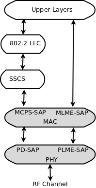
Architecture and scope of lr-wpan models
The grey areas in the figure (adapted from Fig 3. of IEEE Std. 802.15.4-2006) show the scope of the model.
The Spectrum NetDevice from Nicola Baldo is the basis for the implementation.
The implementation also plans to borrow from the ns-2 models developed by Zheng and Lee in the future.
APIs
The APIs closely follow the standard, adapted for ns-3 naming conventions and idioms. The APIs are organized around the concept of service primitives as shown in the following figure adapted from Figure 14 of IEEE Std. 802.15.4-2006.
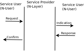
Service primitives
The APIs are organized around four conceptual services and service access points (SAP):
- MAC data service (MCPS)
- MAC management service (MLME)
- PHY data service (PD)
- PHY management service (PLME)
In general, primitives are standardized as follows (e.g. Sec 7.1.1.1.1 of IEEE 802.15.4-2006)::
MCPS-DATA.request      (
                        SrcAddrMode,
                        DstAddrMode,
                        DstPANId,
                        DstAddr,
                        msduLength,
                        msdu,
                        msduHandle,
                        TxOptions,
                        SecurityLevel,
                        KeyIdMode,
                        KeySource,
                        KeyIndex
                        )
This maps to ns-3 classes and methods such as::
struct McpsDataRequestParameters
{
  uint8_t m_srcAddrMode;
  uint8_t m_dstAddrMode;
  ...
};

void
LrWpanMac::McpsDataRequest (McpsDataRequestParameters params)
{
...
}
MAC
The MAC at present implements the unslotted CSMA/CA variant, without beaconing. Currently there is no support for coordinators and the relevant APIs.
The implemented MAC is similar to Contiki’s NullMAC, i.e., a MAC without sleep features. The radio is assumed to be always active (receiving or transmitting), of completely shut down. Frame reception is not disabled while performing the CCA.
The main API supported is the data transfer API (McpsDataRequest/Indication/Confirm). CSMA/CA according to Stc 802.15.4-2006, section 7.5.1.4 is supported. Frame reception and rejection according to Std 802.15.4-2006, section 7.5.6.2 is supported, including acknowledgements. Only short addressing completely implemented. Various trace sources are supported, and trace sources can be hooked to sinks.
PHY
The physical layer components consist of a Phy model, an error rate model, and a loss model. The error rate model presently models the error rate for IEEE 802.15.4 2.4 GHz AWGN channel for OQPSK; the model description can be found in IEEE Std 802.15.4-2006, section E.4.1.7. The Phy model is based on SpectrumPhy and it follows specification described in section 6 of IEEE Std 802.15.4-2006. It models PHY service specifications, PPDU formats, PHY constants and PIB attributes. It currently only supports the transmit power spectral density mask specified in 2.4 GHz per section 6.5.3.1. The noise power density assumes uniformly distributed thermal noise across the frequency bands. The loss model can fully utilize all existing simple (non-spectrum phy) loss models. The Phy model uses the existing single spectrum channel model. The physical layer is modeled on packet level, that is, no preamble/SFD detection is done. Packet reception will be started with the first bit of the preamble (which is not modeled), if the SNR is more than -5 dB, see IEEE Std 802.15.4-2006, appendix E, Figure E.2. Reception of the packet will finish after the packet was completely transmitted. Other packets arriving during reception will add up to the interference/noise.
Currently the receiver sensitivity is set to a fixed value of -106.58 dBm. This corresponds to a packet error rate of 1% for 20 byte reference packets for this signal power, according to IEEE Std 802.15.4-2006, section 6.1.7. In the future we will provide support for changing the sensitivity to different values.
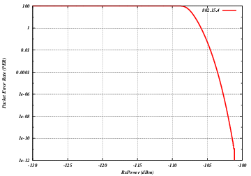
Packet error rate vs. signal power
NetDevice
Although it is expected that other technology profiles (such as 6LoWPAN and ZigBee) will write their own NetDevice classes, a basic LrWpanNetDevice is provided, which encapsulates the common operations of creating a generic LrWpan device and hooking things together.
MAC addresses
Contrary to other technologies, a IEEE 802.15.4 has 2 different kind of addresses:
- Long addresses (64 bits)
- Short addresses (16 bits)
The 64-bit addresses are unique worldwide, and set by the device vendor (in a real device). The 16-bit addresses are not guaranteed to be unique, and they are typically either assigned during the devices deployment, or assigned dynamically during the device bootstrap.
In ns-3 the device bootstrap is not (yet) present. Hence, both addresses are set when the device is created.
The other relavant “address” to consider is the PanId (16 bits), which represents the PAN the device is attached to.
Due to the limited number of available bytes in a packet, IEEE 802.15.4 tries to use short addresses instead of long addresses, even though the two might be used at the same time.
For the sake of communicating with the upper layers, and in particular to generate auto-configured IPv6 addresses, each NetDevice must identify itself with a MAC address. The MAC addresses are also used during packet reception, so it is important to use them consistently.
Focusing on IPv6 Stateless address autoconfiguration (SLAAC), there are two relevant RFCs to consider: RFC 4944 and RFC 6282, and the two differ on how to build the IPv6 address given the NetDevice address.
RFC 4944 mandates that the IID part of the IPv6 address is calculated as YYYY:00ff:fe00:XXXX,
while RFC 6282 mandates that the IID part of the IPv6 address is calculated as 0000:00ff:fe00:XXXX
where XXXX is the device short address, and YYYY is the PanId.
In both cases the U/L bit must be set to local, so in the RFC 4944 the PanId might have one bit flipped.
In order to facilitate interoperability, and to avoid unwanted module dependencies, the ns-3
implementation moves the IID calculation in the LrWpanNetDevice::GetAddress (), which will
return an Address formatted properly, i.e.:
- The Long address (a
Mac64Address) if the Short address has not been set, or - A properly formatted 48-bit pseudo-address (a
Mac48Address) if the short address has been set.
The 48-bit pseudo-address is generated according to either RFC 4944 or RFC 6282 depending on the
configuration of an Attribute (PseudoMacAddressMode).
The default is to use RFC 6282 style addresses.
Note that, on reception, a packet might contain either a short or a long address. This is reflected in the upper-layer notification callback, which can contain either the pseudo-address (48 bits) or the long address (64 bit) of the sender.
Note also that RFC 4944 or RFC 6282 are the RFCs defining the IPv6 address compression formats
(HC1 and IPHC respectively). It is defintely not a good idea to either mix devices using different
pseudo-address format or compression types in the same network. This point is further discussed
in the sixlowpan module documentation.
Scope and Limitations
Future versions of this document will contain a PICS proforma similar to Appendix D of IEEE 802.15.4-2006. The current emphasis is on the unslotted mode of 802.15.4 operation for use in Zigbee, and the scope is limited to enabling a single mode (CSMA/CA) with basic data transfer capabilities. Association with PAN coordinators is not yet supported, nor the use of extended addressing. Interference is modeled as AWGN but this is currently not thoroughly tested.
The NetDevice Tx queue is not limited, i.e., packets are never dropped due to queue becoming full. They may be dropped due to excessive transmission retries or channel access failure.
References
- Wireless Medium Access Control (MAC) and Physical Layer (PHY) Specifications for Low-Rate Wireless Personal Area Networks (WPANs), IEEE Computer Society, IEEE Std 802.15.4-2006, 8 September 2006.
- Zheng and Myung J. Lee, “A comprehensive performance study of IEEE 802.15.4,” Sensor Network Operations, IEEE Press, Wiley Interscience, Chapter 4, pp. 218-237, 2006.
Usage
Enabling lr-wpan
Add lr-wpan to the list of modules built with ns-3.
Helper
The helper is patterned after other device helpers. In particular,
tracing (ascii and pcap) is enabled similarly, and enabling of all
lr-wpan log components is performed similarly. Use of the helper
is exemplified in examples/lr-wpan-data.cc. For ascii tracing,
the transmit and receive traces are hooked at the Mac layer.
The default propagation loss model added to the channel, when this helper is used, is the LogDistancePropagationLossModel with default parameters.
Examples
The following examples have been written, which can be found in src/lr-wpan/examples/:
lr-wpan-data.cc: A simple example showing end-to-end data transfer.lr-wpan-error-distance-plot.cc: An example to plot variations of the packet success ratio as a function of distance.lr-wpan-error-model-plot.cc: An example to test the phy.lr-wpan-packet-print.cc: An example to print out the MAC header fields.lr-wpan-phy-test.cc: An example to test the phy.
In particular, the module enables a very simplified end-to-end data
transfer scenario, implemented in lr-wpan-data.cc. The figure
shows a sequence of events that are triggered when the MAC receives
a DataRequest from the higher layer. It invokes a Clear Channel
Assessment (CCA) from the PHY, and if successful, sends the frame
down to the PHY where it is transmitted over the channel and results
in a DataIndication on the peer node.
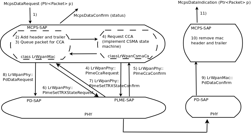
Data example for simple LR-WPAN data transfer end-to-end
The example lr-wpan-error-distance-plot.cc plots the packet success
ratio (PSR) as a function of distance, using the default LogDistance
propagation loss model and the 802.15.4 error model. The channel (default 11),
packet size (default 20 bytes) and transmit power (default 0 dBm) can be
varied by command line arguments. The program outputs a file named
802.15.4-psr-distance.plt. Loading this file into gnuplot yields
a file 802.15.4-psr-distance.eps, which can be converted to pdf or
other formats. The default output is shown below.
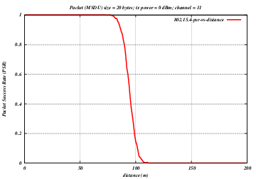
Default output of the program lr-wpan-error-distance-plot.cc
Tests
The following tests have been written, which can be found in src/lr-wpan/tests/:
lr-wpan-ack-test.cc: Check that acknowledgments are being used and issued in the correct order.lr-wpan-collision-test.cc: Test correct reception of packets with interference and collisions.lr-wpan-error-model-test.cc: Check that the error model gives predictable values.lr-wpan-packet-test.cc: Test the 802.15.4 MAC header/trailer classeslr-wpan-pd-plme-sap-test.cc: Test the PLME and PD SAP per IEEE 802.15.4lr-wpan-spectrum-value-helper-test.cc: Test that the conversion between power (expressed as a scalar quantity) and spectral power, and back again, falls within a 25% tolerance across the range of possible channels and input powers.
Validation
The model has not been validated against real hardware. The error model
has been validated against the data in IEEE Std 802.15.4-2006,
section E.4.1.7 (Figure E.2). The MAC behavior (CSMA backoff) has been
validated by hand against expected behavior. The below plot is an example
of the error model validation and can be reproduced by running
lr-wpan-error-model-plot.cc:
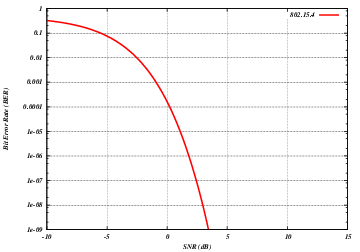
Default output of the program lr-wpan-error-model-plot.cc
LTE Module
Design Documentation
Overview
An overview of the LTE-EPC simulation model is depicted in the figure Overview of the LTE-EPC simulation model. There are two main components:
- the LTE Model. This model includes the LTE Radio Protocol stack (RRC, PDCP, RLC, MAC, PHY). These entities reside entirely within the UE and the eNB nodes.
- the EPC Model. This model includes core network interfaces, protocols and entities. These entities and protocols reside within the SGW, PGW and MME nodes, and partially within the eNB nodes.
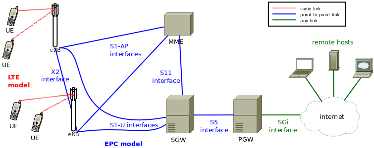
Overview of the LTE-EPC simulation model
Design Criteria
LTE Model
The LTE model has been designed to support the evaluation of the following aspects of LTE systems:
- Radio Resource Management
- QoS-aware Packet Scheduling
- Inter-cell Interference Coordination
- Dynamic Spectrum Access
In order to model LTE systems to a level of detail that is sufficient to allow a correct evaluation of the above mentioned aspects, the following requirements have been considered:
- At the radio level, the granularity of the model should be at least that of the Resource Block (RB). In fact, this is the fundamental unit being used for resource allocation. Without this minimum level of granularity, it is not possible to model accurately packet scheduling and inter-cell-interference. The reason is that, since packet scheduling is done on a per-RB basis, an eNB might transmit on a subset only of all the available RBs, hence interfering with other eNBs only on those RBs where it is transmitting. Note that this requirement rules out the adoption of a system level simulation approach, which evaluates resource allocation only at the granularity of call/bearer establishment.
- The simulator should scale up to tens of eNBs and hundreds of User Equipment (UEs). This rules out the use of a link level simulator, i.e., a simulator whose radio interface is modeled with a granularity up to the symbol level. This is because to have a symbol level model it is necessary to implement all the PHY layer signal processing, whose huge computational complexity severely limits simulation. In fact, link-level simulators are normally limited to a single eNB and one or a few UEs.
- It should be possible within the simulation to configure different cells so that they use different carrier frequencies and system bandwidths. The bandwidth used by different cells should be allowed to overlap, in order to support dynamic spectrum licensing solutions such as those described in [Ofcom2600MHz] and [RealWireless]. The calculation of interference should handle appropriately this case.
- To be more representative of the LTE standard, as well as to be as close as possible to real-world implementations, the simulator should support the MAC Scheduler API published by the FemtoForum [FFAPI]. This interface is expected to be used by femtocell manufacturers for the implementation of scheduling and Radio Resource Management (RRM) algorithms. By introducing support for this interface in the simulator, we make it possible for LTE equipment vendors and operators to test in a simulative environment exactly the same algorithms that would be deployed in a real system.
- The LTE simulation model should contain its own implementation of the API defined in [FFAPI]. Neither binary nor data structure compatibility with vendor-specific implementations of the same interface are expected; hence, a compatibility layer should be interposed whenever a vendor-specific MAC scheduler is to be used with the simulator. This requirement is necessary to allow the simulator to be independent from vendor-specific implementations of this interface specification. We note that [FFAPI] is a logical specification only, and its implementation (e.g., translation to some specific programming language) is left to the vendors.
- The model is to be used to simulate the transmission of IP packets by the upper layers. With this respect, it shall be considered that in LTE the Scheduling and Radio Resource Management do not work with IP packets directly, but rather with RLC PDUs, which are obtained by segmentation and concatenation of IP packets done by the RLC entities. Hence, these functionalities of the RLC layer should be modeled accurately.
EPC Model
The main objective of the EPC model is to provides means for the simulation of end-to-end IP connectivity over the LTE model. To this aim, it supports for the interconnection of multiple UEs to the Internet, via a radio access network of multiple eNBs connected to the core network, as shown in Figure Overview of the LTE-EPC simulation model.
The following design choices have been made for the EPC model:
- The Packet Data Network (PDN) type supported is both IPv4 and IPv6. In other words, the end-to-end connections between the UEs and the remote hosts can be IPv4 and IPv6. However, the networks between the core network elements (MME, SGWs and PGWs) are IPv4-only.
- The SGW and PGW functional entities are implemented in different nodes, which are hence referred to as the SGW node and PGW node, respectively.
- The MME functional entities is implemented as a network node, which is hence referred to as the MME node.
- The scenarios with inter-SGW mobility are not of interest. But several SGW nodes may be present in simulations scenarios.
- A requirement for the EPC model is that it can be used to simulate the end-to-end performance of realistic applications. Hence, it should be possible to use with the EPC model any regular ns-3 application working on top of TCP or UDP.
- Another requirement is the possibility of simulating network topologies with the presence of multiple eNBs, some of which might be equipped with a backhaul connection with limited capabilities. In order to simulate such scenarios, the user data plane protocols being used between the eNBs and the SGW should be modeled accurately.
- It should be possible for a single UE to use different applications with different QoS profiles. Hence, multiple EPS bearers should be supported for each UE. This includes the necessary classification of TCP/UDP traffic over IP done at the UE in the uplink and at the PGW in the downlink.
- The initial focus of the EPC model is mainly on the EPC data plane. The accurate modeling of the EPC control plane is, for the time being, not a requirement; however, the necessary control plane interactions among the different network nodes of the core network are realized by implementing control protocols/messages among them. Direct interaction among the different simulation objects via the provided helper objects should be avoided as much as possible.
- The focus of the EPC model is on simulations of active users in ECM connected mode. Hence, all the functionality that is only relevant for ECM idle mode (in particular, tracking area update and paging) are not modeled at all.
- The model should allow the possibility to perform an X2-based handover between two eNBs.
Architecture
LTE Model
UE architecture
The architecture of the LTE radio protocol stack model of the UE is represented in the figures LTE radio protocol stack architecture for the UE on the data plane and LTE radio protocol stack architecture for the UE on the control plane which highlight respectively the data plane and the control plane.
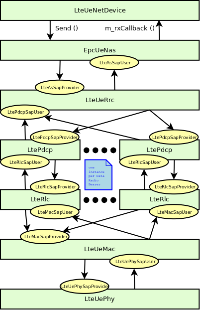
LTE radio protocol stack architecture for the UE on the data plane
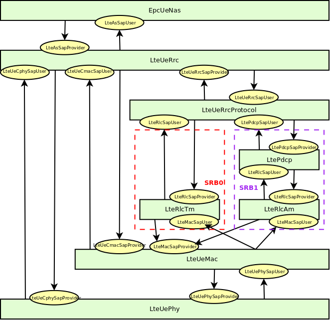
LTE radio protocol stack architecture for the UE on the control plane
The architecture of the PHY/channel model of the UE is represented in figure PHY and channel model architecture for the UE.
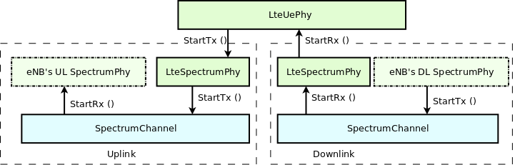
PHY and channel model architecture for the UE
eNB architecture
The architecture of the LTE radio protocol stack model of the eNB is represented in the figures LTE radio protocol stack architecture for the eNB on the data plane and LTE radio protocol stack architecture for the eNB on the control plane which highlight respectively the data plane and the control plane.
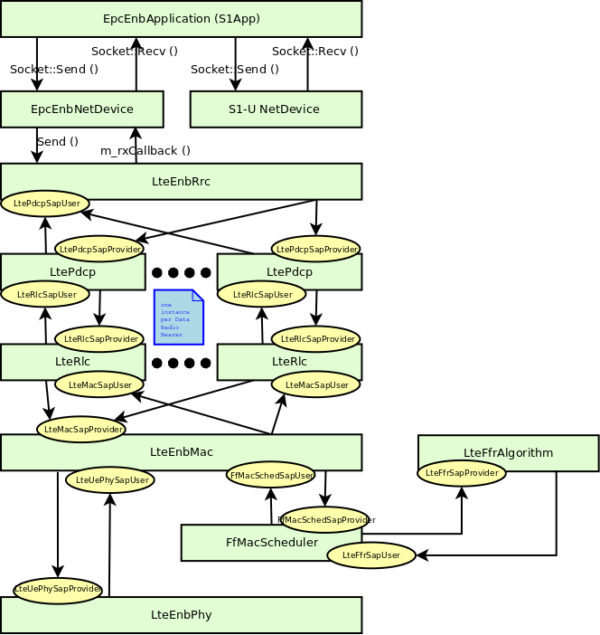
LTE radio protocol stack architecture for the eNB on the data plane
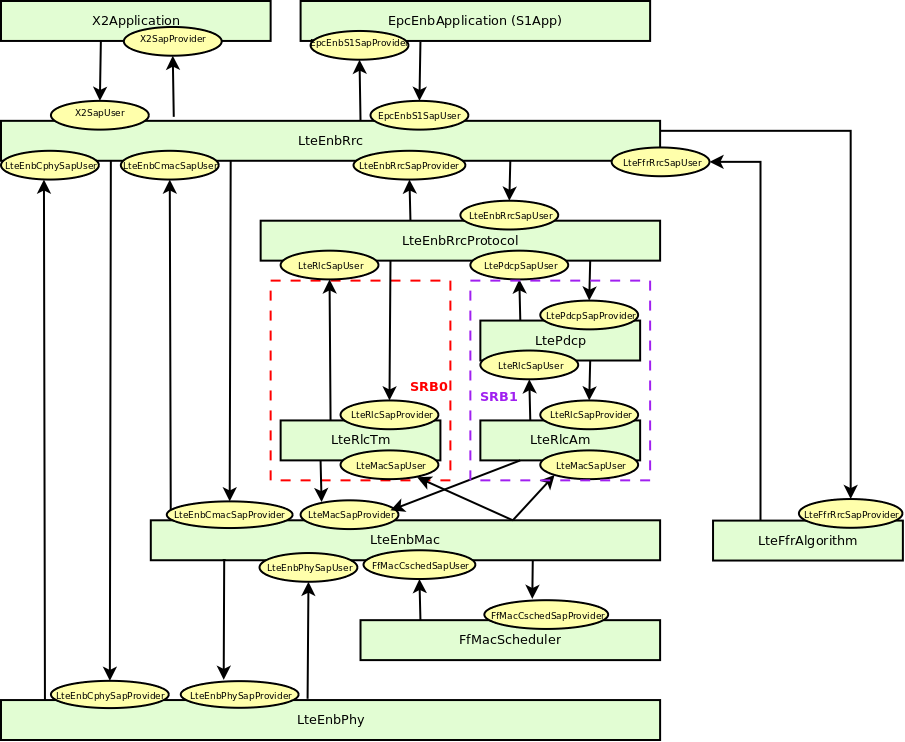
LTE radio protocol stack architecture for the eNB on the control plane
The architecture of the PHY/channel model of the eNB is represented in figure PHY and channel model architecture for the eNB.
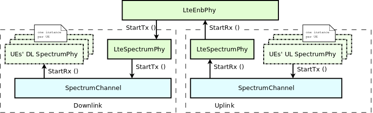
PHY and channel model architecture for the eNB
EPC Model
EPC data plane
In Figure LTE-EPC data plane protocol stack, we represent the end-to-end LTE-EPC data plane protocol stack as it is modeled in the simulator. The figure shows all nodes in the data path, i.e. UE, eNB, SGW, PGW and a remote host in the Internet. All protocol stacks (S5 protocol stack, S1-U protocol stack and the LTE radio protocol stack) specified by 3GPP are present.
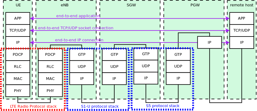
LTE-EPC data plane protocol stack
EPC control plane
The architecture of the implementation of the control plane model is shown in figure LTE-EPC control plane protocol stack. The control interfaces that are modeled explicitly are the S1-MME, the S11, and the S5 interfaces. The X2 interface is also modeled explicitly and it is described in more detail in section X2
The S1-MME, the S11 and the S5 interfaces are modeled using procotol data units sent over its respective links. These interfaces use the SCTP protocol as transport protocol but currently, the SCTP protocol is not modeled in the ns-3 simulator, so the UDP protocol is used instead of the SCTP protocol.
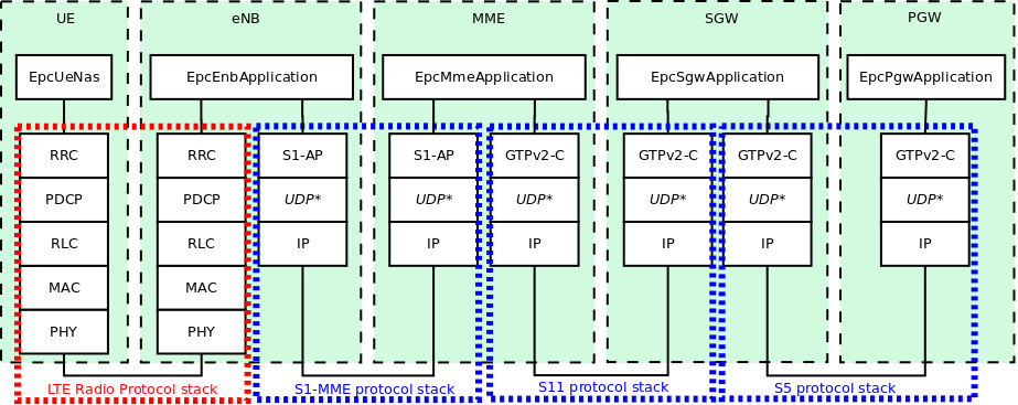
LTE-EPC control plane protocol stack
Channel and Propagation
For channel modeling purposes, the LTE module uses the SpectrumChannel
interface provided by the spectrum module. At the time of this
writing, two implementations of such interface are available:
SingleModelSpectrumChannel and MultiModelSpectrumChannel, and the
LTE module requires the use of the MultiModelSpectrumChannel in
order to work properly. This is because of the need to support
different frequency and bandwidth configurations. All the
propagation models supported by MultiModelSpectrumChannel can be
used within the LTE module.
Use of the Buildings model with LTE
The recommended propagation model to be used with the LTE module is the one provided by the Buildings module, which was in fact designed specifically with LTE (though it can be used with other wireless technologies as well). Please refer to the documentation of the Buildings module for generic information on the propagation model it provides.
In this section we will highlight some considerations that specifically apply when the Buildings module is used together with the LTE module.
The naming convention used in the following will be:
- User equipment: UE
- Macro Base Station: MBS
- Small cell Base Station (e.g., pico/femtocell): SC
The LTE module considers FDD only, and implements downlink and uplink propagation separately. As a consequence, the following pathloss computations are performed
- MBS <-> UE (indoor and outdoor)
- SC (indoor and outdoor) <-> UE (indoor and outdoor)
The LTE model does not provide the following pathloss computations:
- UE <-> UE
- MBS <-> MBS
- MBS <-> SC
- SC <-> SC
The Buildings model does not know the actual type of the node; i.e., it is not aware of whether a transmitter node is a UE, a MBS, or a SC. Rather, the Buildings model only cares about the position of the node: whether it is indoor and outdoor, and what is its z-axis respect to the rooftop level. As a consequence, for an eNB node that is placed outdoor and at a z-coordinate above the rooftop level, the propagation models typical of MBS will be used by the Buildings module. Conversely, for an eNB that is placed outdoor but below the rooftop, or indoor, the propagation models typical of pico and femtocells will be used.
For communications involving at least one indoor node, the corresponding wall penetration losses will be calculated by the Buildings model. This covers the following use cases:
- MBS <-> indoor UE
- outdoor SC <-> indoor UE
- indoor SC <-> indoor UE
- indoor SC <-> outdoor UE
Please refer to the documentation of the Buildings module for details on the actual models used in each case.
Fading Model
The LTE module includes a trace-based fading model derived from the one developed during the GSoC 2010 [Piro2011]. The main characteristic of this model is the fact that the fading evaluation during simulation run-time is based on per-calculated traces. This is done to limit the computational complexity of the simulator. On the other hand, it needs huge structures for storing the traces; therefore, a trade-off between the number of possible parameters and the memory occupancy has to be found. The most important ones are:
- users’ speed: relative speed between users (affects the Doppler frequency, which in turns affects the time-variance property of the fading)
- number of taps (and relative power): number of multiple paths considered, which affects the frequency property of the fading.
- time granularity of the trace: sampling time of the trace.
- frequency granularity of the trace: number of values in frequency to be evaluated.
- length of trace: ideally large as the simulation time, might be reduced by windowing mechanism.
- number of users: number of independent traces to be used (ideally one trace per user).
With respect to the mathematical channel propagation model, we suggest the one provided by the rayleighchan function of Matlab, since it provides a well accepted channel modelization both in time and frequency domain. For more information, the reader is referred to [mathworks].
The simulator provides a matlab script (src/lte/model/fading-traces/fading-trace-generator.m) for generating traces based on the format used by the simulator.
In detail, the channel object created with the rayleighchan function is used for filtering a discrete-time impulse signal in order to obtain the channel impulse response. The filtering is repeated for different TTI, thus yielding subsequent time-correlated channel responses (one per TTI). The channel response is then processed with the pwelch function for obtaining its power spectral density values, which are then saved in a file with the proper format compatible with the simulator model.
Since the number of variable it is pretty high, generate traces considering all of them might produce a high number of traces of huge size. On this matter, we considered the following assumptions of the parameters based on the 3GPP fading propagation conditions (see Annex B.2 of [TS36104]):
- users’ speed: typically only a few discrete values are considered, i.e.:
- 0 and 3 kmph for pedestrian scenarios
- 30 and 60 kmph for vehicular scenarios
- 0, 3, 30 and 60 for urban scenarios
- channel taps: only a limited number of sets of channel taps are normally considered, for example three models are mentioned in Annex B.2 of [TS36104].
- time granularity: we need one fading value per TTI, i.e., every 1 ms (as this is the granularity in time of the ns-3 LTE PHY model).
- frequency granularity: we need one fading value per RB (which is the frequency granularity of the spectrum model used by the ns-3 LTE model).
- length of the trace: the simulator includes the windowing mechanism implemented during the GSoC 2011, which consists of picking up a window of the trace each window length in a random fashion.
- per-user fading process: users share the same fading trace, but for each user a different starting point in the trace is randomly picked up. This choice was made to avoid the need to provide one fading trace per user.
According to the parameters we considered, the following formula express in detail the total size  of the fading traces:
![S_{traces} = S_{sample} \times N_{RB} \times \frac{T_{trace}}{T_{sample}} \times N_{scenarios} \mbox{ [bytes]}](_images/math/812b0ae58acce66e756b3058479ec683c1b41748.png)
where  is the size in bytes of the sample (e.g., 8 in case of double precision, 4 in case of float precision),
  is the number of RB or set of RBs to be considered,
  is the total length of the trace,
  is the time resolution of the trace (1 ms), and
  is the number of fading scenarios that are desired (i.e., combinations of different sets of channel taps and user speed values). We provide traces for 3 different scenarios one for each taps configuration defined in Annex B.2 of [TS36104]:
- Pedestrian: with nodes’ speed of 3 kmph.
- Vehicular: with nodes’ speed of 60 kmph.
- Urban: with nodes’ speed of 3 kmph.
hence 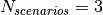 . All traces have
  s and
s and  . This results in a total 24 MB bytes of traces.
Antennas
Being based on the SpectrumPhy, the LTE PHY model supports antenna
modeling via the ns-3 AntennaModel class. Hence, any model based on
this class can be associated with any eNB or UE instance. For
instance, the use of the CosineAntennaModel associated with an eNB
device allows to model one sector of a macro base station. By default,
the IsotropicAntennaModel is used for both eNBs and UEs.
PHY
Overview
The physical layer model provided in this LTE simulator is based on the one described in [Piro2011], with the following modifications. The model now includes the inter cell interference calculation and the simulation of uplink traffic, including both packet transmission and CQI generation.
Subframe Structure
The subframe is divided into control and data part as described in Figure LTE subframe division..
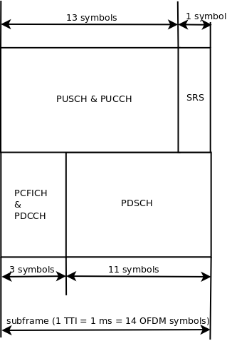
LTE subframe division.
Considering the granularity of the simulator based on RB, the control and the reference signaling have to be consequently modeled considering this constraint. According to the standard [TS36211], the downlink control frame starts at the beginning of each subframe and lasts up to three symbols across the whole system bandwidth, where the actual duration is provided by the Physical Control Format Indicator Channel (PCFICH). The information on the allocation are then mapped in the remaining resource up to the duration defined by the PCFICH, in the so called Physical Downlink Control Channel (PDCCH). A PDCCH transports a single message called Downlink Control Information (DCI) coming from the MAC layer, where the scheduler indicates the resource allocation for a specific user. The PCFICH and PDCCH are modeled with the transmission of the control frame of a fixed duration of 3/14 of milliseconds spanning in the whole available bandwidth, since the scheduler does not estimate the size of the control region. This implies that a single transmission block models the entire control frame with a fixed power (i.e., the one used for the PDSCH) across all the available RBs. According to this feature, this transmission represents also a valuable support for the Reference Signal (RS). This allows of having every TTI an evaluation of the interference scenario since all the eNB are transmitting (simultaneously) the control frame over the respective available bandwidths. We note that, the model does not include the power boosting since it does not reflect any improvement in the implemented model of the channel estimation.
The Sounding Reference Signal (SRS) is modeled similar to the downlink control frame. The SRS is periodically placed in the last symbol of the subframe in the whole system bandwidth. The RRC module already includes an algorithm for dynamically assigning the periodicity as function of the actual number of UEs attached to a eNB according to the UE-specific procedure (see Section 8.2 of [TS36213]).
MAC to Channel delay
To model the latency of real MAC and PHY implementations, the PHY model simulates a MAC-to-channel delay in multiples of TTIs (1ms). The transmission of both data and control packets are delayed by this amount.
CQI feedback
The generation of CQI feedback is done accordingly to what specified in [FFAPI]. In detail, we considered the generation of periodic wideband CQI (i.e., a single value of channel state that is deemed representative of all RBs in use) and inband CQIs (i.e., a set of value representing the channel state for each RB).
The CQI index to be reported is obtained by first obtaining a SINR measurement and then passing this SINR measurement to the Adaptive Modulation and Coding module which will map it to the CQI index.
In downlink, the SINR used to generate CQI feedback can be calculated in two different ways:
- Ctrl method: SINR is calculated combining the signal power from the reference signals (which in the simulation is equivalent to the PDCCH) and the interference power from the PDCCH. This approach results in considering any neighboring eNB as an interferer, regardless of whether this eNB is actually performing any PDSCH transmission, and regardless of the power and RBs used for eventual interfering PDSCH transmissions.
- Mixed method: SINR is calculated combining the signal power from the reference signals (which in the simulation is equivalent to the PDCCH) and the interference power from the PDSCH. This approach results in considering as interferers only those neighboring eNBs that are actively transmitting data on the PDSCH, and allows to generate inband CQIs that account for different amounts of interference on different RBs according to the actual interference level. In the case that no PDSCH transmission is performed by any eNB, this method consider that interference is zero, i.e., the SINR will be calculated as the ratio of signal to noise only.
To switch between this two CQI generation approaches, LteHelper::UsePdschForCqiGeneration needs to be configured: false for first approach and true for second approach (true is default value):
Config::SetDefault ("ns3::LteHelper::UsePdschForCqiGeneration", BooleanValue (true));
In uplink, two types of CQIs are implemented:
- SRS based, periodically sent by the UEs.
- PUSCH based, calculated from the actual transmitted data.
The scheduler interface include an attribute system called UlCqiFilter for managing the filtering of the CQIs according to their nature, in detail:
SRS_UL_CQIfor storing only SRS based CQIs.PUSCH_UL_CQIfor storing only PUSCH based CQIs.
It has to be noted that, the FfMacScheduler provides only the interface and it is matter of the actual scheduler implementation to include the code for managing these attributes (see scheduler related section for more information on this matter).
Interference Model
The PHY model is based on the well-known Gaussian interference models, according to which the powers of interfering signals (in linear units) are summed up together to determine the overall interference power.
The sequence diagram of Figure Sequence diagram of the PHY interference calculation procedure shows how interfering signals are processed to calculate the SINR, and how SINR is then used for the generation of CQI feedback.
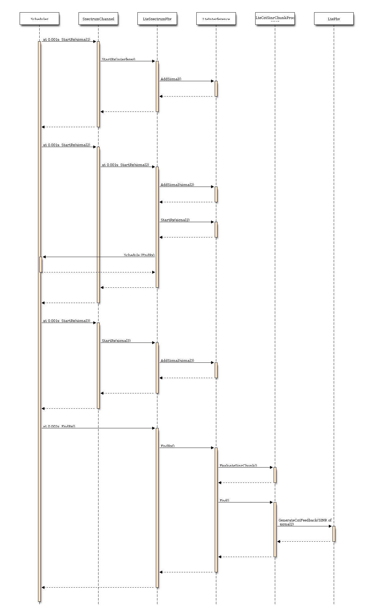
Sequence diagram of the PHY interference calculation procedure
LTE Spectrum Model
The usage of the radio spectrum by eNBs and UEs in LTE is described in
[TS36101]. In the simulator, radio spectrum usage is modeled as follows.
Let  denote the LTE Absolute Radio Frequency Channel Number, which
identifies the carrier frequency on a 100 kHz raster; furthermore, let
denote the LTE Absolute Radio Frequency Channel Number, which
identifies the carrier frequency on a 100 kHz raster; furthermore, let  be
the Transmission Bandwidth Configuration in number of Resource Blocks. For every
pair
be
the Transmission Bandwidth Configuration in number of Resource Blocks. For every
pair  used in the simulation we define a corresponding SpectrumModel using
the functionality provided by the Spectrum Module .
model using the Spectrum framework described
in [Baldo2009]. and can be configured for every eNB instantiated
in the simulation; hence, each eNB can use a different spectrum model. Every UE
will automatically use the spectrum model of the eNB it is attached to. Using
the MultiModelSpectrumChannel described in [Baldo2009], the interference
among eNBs that use different spectrum models is properly accounted for.
This allows to simulate dynamic spectrum access policies, such as for
example the spectrum licensing policies that are
discussed in [Ofcom2600MHz].
used in the simulation we define a corresponding SpectrumModel using
the functionality provided by the Spectrum Module .
model using the Spectrum framework described
in [Baldo2009]. and can be configured for every eNB instantiated
in the simulation; hence, each eNB can use a different spectrum model. Every UE
will automatically use the spectrum model of the eNB it is attached to. Using
the MultiModelSpectrumChannel described in [Baldo2009], the interference
among eNBs that use different spectrum models is properly accounted for.
This allows to simulate dynamic spectrum access policies, such as for
example the spectrum licensing policies that are
discussed in [Ofcom2600MHz].
Data PHY Error Model
The simulator includes an error model of the data plane (i.e., PDSCH and PUSCH) according to the standard link-to-system mapping (LSM) techniques. The choice is aligned with the standard system simulation methodology of OFDMA radio transmission technology. Thanks to LSM we are able to maintain a good level of accuracy and at the same time limiting the computational complexity increase. It is based on the mapping of single link layer performance obtained by means of link level simulators to system (in our case network) simulators. In particular link the layer simulator is used for generating the performance of a single link from a PHY layer perspective, usually in terms of code block error rate (BLER), under specific static conditions. LSM allows the usage of these parameters in more complex scenarios, typical of system/network simulators, where we have more links, interference and “colored” channel propagation phenomena (e.g., frequency selective fading).
To do this the Vienna LTE Simulator [ViennaLteSim] has been used for what concerns the extraction of link layer performance and the Mutual Information Based Effective SINR (MIESM) as LSM mapping function using part of the work recently published by the Signet Group of University of Padua [PaduaPEM].
MIESM
The specific LSM method adopted is the one based on the usage of a mutual information metric, commonly referred to as the mutual information per per coded bit (MIB or MMIB when a mean of multiples MIBs is involved). Another option would be represented by the Exponential ESM (EESM); however, recent studies demonstrate that MIESM outperforms EESM in terms of accuracy [LozanoCost].
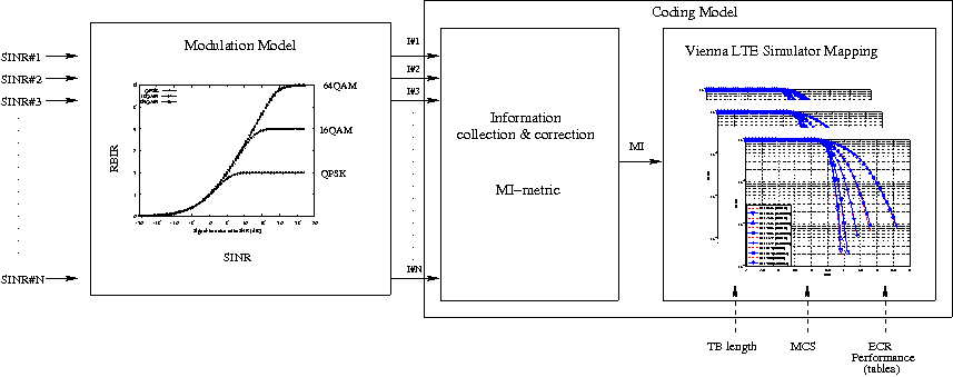
MIESM computational procedure diagram
The mutual information (MI) is dependent on the constellation mapping and can be calculated per transport block (TB) basis, by evaluating the MI over the symbols and the subcarrier. However, this would be too complex for a network simulator. Hence, in our implementation a flat channel response within the RB has been considered; therefore the overall MI of a TB is calculated averaging the MI evaluated per each RB used in the TB. In detail, the implemented scheme is depicted in Figure MIESM computational procedure diagram, where we see that the model starts by evaluating the MI value for each RB, represented in the figure by the SINR samples. Then the equivalent MI is evaluated per TB basis by averaging the MI values. Finally, a further step has to be done since the link level simulator returns the performance of the link in terms of block error rate (BLER) in a addive white gaussian noise (AWGN) channel, where the blocks are the code blocks (CBs) independently encoded/decoded by the turbo encoder. On this matter the
standard 3GPP segmentation scheme has been used for estimating the actual CB size (described in section 5.1.2 of [TS36212]). This scheme divides the TB in  blocks of size
  and
and  blocks of size
  . Therefore the overall TB BLER (TBLER) can be expressed as
where the  is the BLER of the CB
  obtained according to the link level simulator CB BLER curves.
For estimating the , the MI evaluation has been implemented according to its numerical approximation defined in [wimaxEmd]. Moreover, for reducing the complexity of the computation, the approximation has been converted into lookup tables. In detail, Gaussian cumulative model has been used for approximating the AWGN BLER curves with three parameters which provides a close fit to the standard AWGN performances, in formula:
obtained according to the link level simulator CB BLER curves.
For estimating the , the MI evaluation has been implemented according to its numerical approximation defined in [wimaxEmd]. Moreover, for reducing the complexity of the computation, the approximation has been converted into lookup tables. In detail, Gaussian cumulative model has been used for approximating the AWGN BLER curves with three parameters which provides a close fit to the standard AWGN performances, in formula:
![CBLER_i = \frac{1}{2}\left[1-erf\left(\frac{x-b_{ECR}}{\sqrt{2}c_{ECR}} \right) \right]](_images/math/dad7d004bf7aa9c347fe674e6e142a7b3d54da1c.png)
where is the MI of the TB,  represents the “transition center” and
  is related to the “transition width” of the Gaussian cumulative distribution for each Effective Code Rate (ECR) which is the actual transmission rate according to the channel coding and MCS. For limiting the computational complexity of the model we considered only a subset of the possible ECRs in fact we would have potentially 5076 possible ECRs (i.e., 27 MCSs and 188 CB sizes). On this respect, we will limit the CB sizes to some representative values (i.e., 40, 140, 160, 256, 512, 1024, 2048, 4032, 6144), while for the others the worst one approximating the real one will be used (i.e., the smaller CB size value available respect to the real one). This choice is aligned to the typical performance of turbo codes, where the CB size is not strongly impacting on the BLER. However, it is to be notes that for CB sizes lower than 1000 bits the effect might be relevant (i.e., till 2 dB); therefore, we adopt
this unbalanced sampling interval for having more precision where it is necessary. This behaviour is confirmed by the figures presented in the Annes Section.
is related to the “transition width” of the Gaussian cumulative distribution for each Effective Code Rate (ECR) which is the actual transmission rate according to the channel coding and MCS. For limiting the computational complexity of the model we considered only a subset of the possible ECRs in fact we would have potentially 5076 possible ECRs (i.e., 27 MCSs and 188 CB sizes). On this respect, we will limit the CB sizes to some representative values (i.e., 40, 140, 160, 256, 512, 1024, 2048, 4032, 6144), while for the others the worst one approximating the real one will be used (i.e., the smaller CB size value available respect to the real one). This choice is aligned to the typical performance of turbo codes, where the CB size is not strongly impacting on the BLER. However, it is to be notes that for CB sizes lower than 1000 bits the effect might be relevant (i.e., till 2 dB); therefore, we adopt
this unbalanced sampling interval for having more precision where it is necessary. This behaviour is confirmed by the figures presented in the Annes Section.
BLER Curves
On this respect, we reused part of the curves obtained within [PaduaPEM]. In detail, we introduced the CB size dependency to the CB BLER curves with the support of the developers of [PaduaPEM] and of the LTE Vienna Simulator. In fact, the module released provides the link layer performance only for what concerns the MCSs (i.e, with a given fixed ECR). In detail the new error rate curves for each has been evaluated with a simulation campaign with the link layer simulator for a single link with AWGN noise and for CB size of 104, 140, 256, 512, 1024, 2048, 4032 and 6144. These curves has been mapped with the Gaussian cumulative model formula presented above for obtaining the correspondents and parameters.
The BLER performance of all MCS obtained with the link level simulator are plotted in the following figures (blue lines) together with their correspondent mapping to the Gaussian cumulative distribution (red dashed lines).
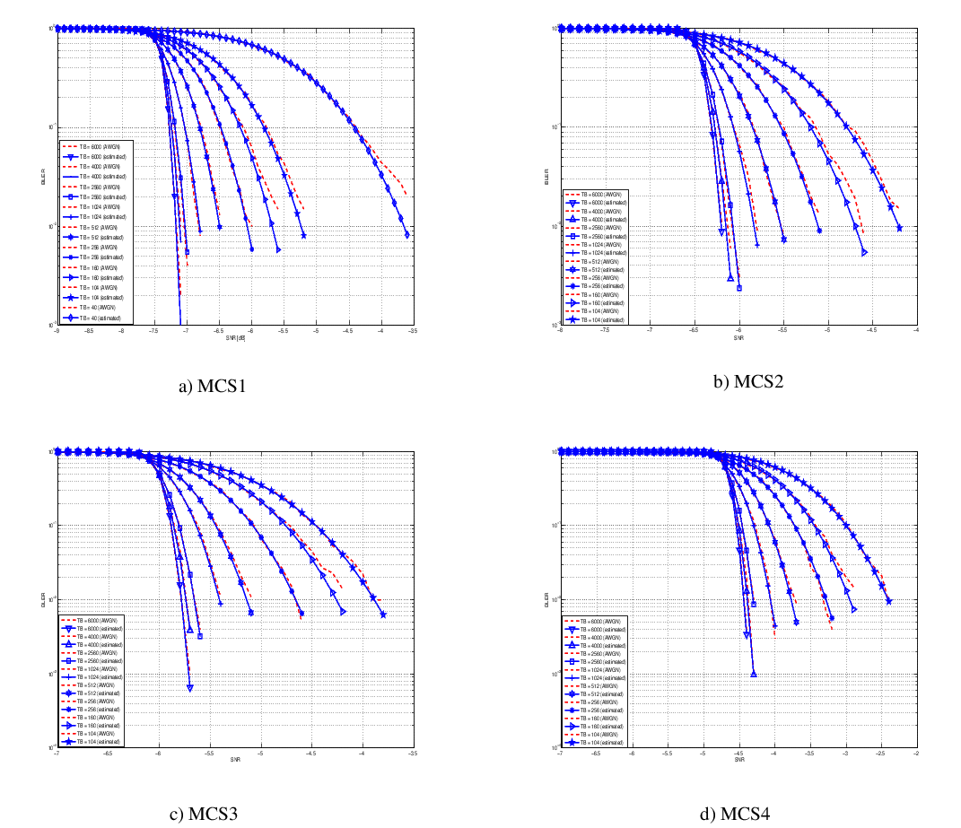
BLER for MCS 1, 2, 3 and 4.
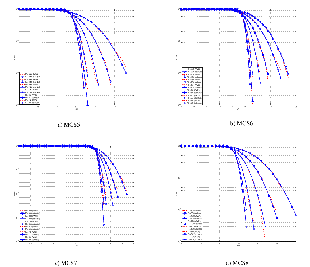
BLER for MCS 5, 6, 7 and 8.
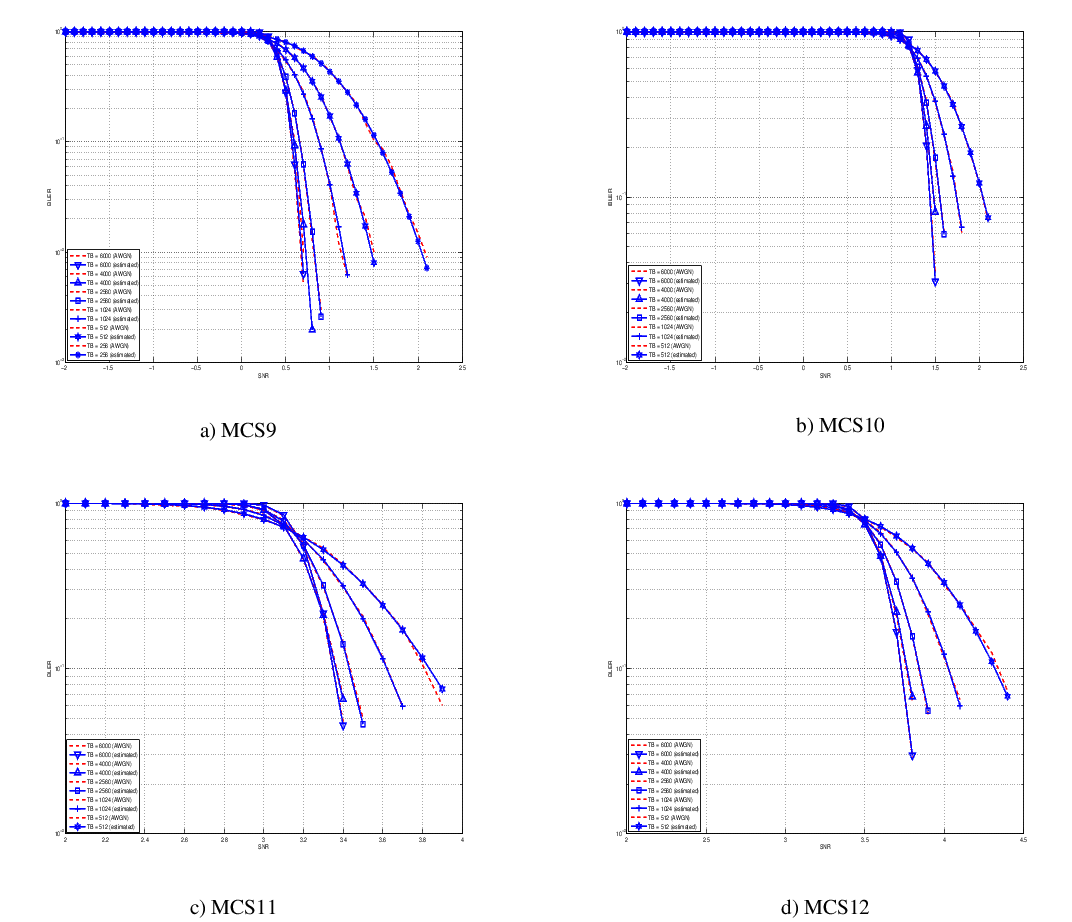
BLER for MCS 9, 10, 11 and 12.
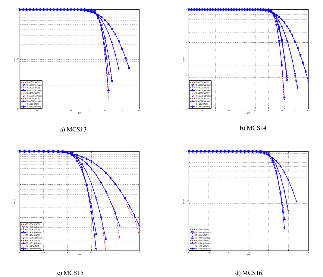
BLER for MCS 13, 14, 15 and 16.
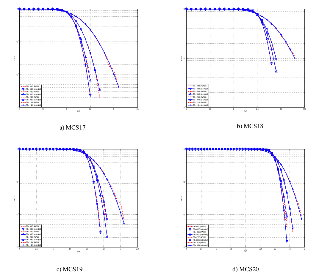
BLER for MCS 17, 17, 19 and 20.
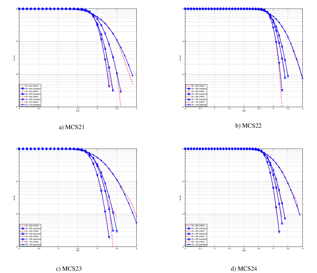
BLER for MCS 21, 22, 23 and 24.
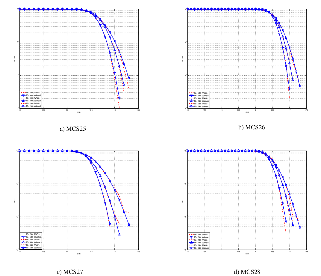
BLER for MCS 25, 26, 27 and 28.
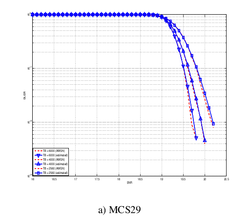
BLER for MCS 29.
Integration of the BLER curves in the ns-3 LTE module
The model implemented uses the curves for the LSM of the recently LTE PHY Error Model released in the ns3 community by the Signet Group [PaduaPEM] and the new ones generated for different CB sizes. The LteSpectrumPhy class is in charge of evaluating the TB BLER thanks to the methods provided by the LteMiErrorModel class, which is in charge of evaluating the TB BLER according to the vector of the perceived SINR per RB, the MCS and the size in order to proper model the segmentation of the TB in CBs. In order to obtain the vector of the perceived SINRs for data and control signals, two instances of LteChunkProcessor (dedicated to evaluate the SINR for obtaining physical error performance) have been attached to UE downlink and eNB uplink LteSpectrumPhy modules for evaluating the error model distribution of PDSCH (UE side) and ULSCH (eNB side).
The model can be disabled for working with a zero-losses channel by setting the DataErrorModelEnabled attribute of the LteSpectrumPhy class (by default is active). This can be done according to the standard ns3 attribute system procedure, that is:
Config::SetDefault ("ns3::LteSpectrumPhy::DataErrorModelEnabled", BooleanValue (false));
Control Channels PHY Error Model
The simulator includes the error model for downlink control channels (PCFICH and PDCCH), while in uplink it is assumed and ideal error-free channel. The model is based on the MIESM approach presented before for considering the effects of the frequency selective channel since most of the control channels span the whole available bandwidth.
PCFICH + PDCCH Error Model
The model adopted for the error distribution of these channels is based on an evaluation study carried out in the RAN4 of 3GPP, where different vendors investigated the demodulation performance of the PCFICH jointly with PDCCH. This is due to the fact that the PCFICH is the channel in charge of communicating to the UEs the actual dimension of the PDCCH (which spans between 1 and 3 symbols); therefore the correct decodification of the DCIs depends on the correct interpretation of both ones. In 3GPP this problem have been evaluated for improving the cell-edge performance [FujitsuWhitePaper], where the interference among neighboring cells can be relatively high due to signal degradation. A similar problem has been notices in femto-cell scenario and, more in general, in HetNet scenarios the bottleneck has been detected mainly as the PCFICH channel [Bharucha2011], where in case of many eNBs are deployed in the same service area, this channel may collide in frequency, making impossible the correct detection of the PDCCH channel, too.
In the simulator, the SINR perceived during the reception has been estimated according to the MIESM model presented above in order to evaluate the error distribution of PCFICH and PDCCH. In detail, the SINR samples of all the RBs are included in the evaluation of the MI associated to the control frame and, according to this values, the effective SINR (eSINR) is obtained by inverting the MI evaluation process. It has to be noted that, in case of MIMO transmission, both PCFICH and the PDCCH use always the transmit diversity mode as defined by the standard. According to the eSINR perceived the decodification error probability can be estimated as function of the results presented in [R4-081920]. In case an error occur, the DCIs discarded and therefore the UE will be not able to receive the correspondent Tbs, therefore resulting lost.
MIMO Model
The use of multiple antennas both at transmitter and receiver side, known as multiple-input and multiple-output (MIMO), is a problem well studied in literature during the past years. Most of the work concentrate on evaluating analytically the gain that the different MIMO schemes might have in term of capacity; however someones provide also information of the gain in terms of received power [CatreuxMIMO].
According to the considerations above, a model more flexible can be obtained considering the gain that MIMO schemes bring in the system from a statistical point of view. As highlighted before, [CatreuxMIMO] presents the statistical gain of several MIMO solutions respect to the SISO one in case of no correlation between the antennas. In the work the gain is presented as the cumulative distribution function (CDF) of the output SINR for what concern SISO, MIMO-Alamouti, MIMO-MMSE, MIMO-OSIC-MMSE and MIMO-ZF schemes. Elaborating the results, the output SINR distribution can be approximated with a log-normal one with different mean and variance as function of the scheme considered. However, the variances are not so different and they are approximatively equal to the one of the SISO mode already included in the shadowing component of the BuildingsPropagationLossModel, in detail:
- SISO:
and
[dB].
- MIMO-Alamouti:
and
[dB].
- MIMO-MMSE:
and
[dB].
- MIMO-OSIC-MMSE:
and
[dB].
- MIMO-ZF:
and
[dB].
Therefore the PHY layer implements the MIMO model as the gain perceived by the receiver when using a MIMO scheme respect to the one obtained using SISO one. We note that, these gains referred to a case where there is no correlation between the antennas in MIMO scheme; therefore do not model degradation due to paths correlation.
UE PHY Measurements Model
According to [TS36214], the UE has to report a set of measurements of the eNBs that the device is able to perceive: the reference signal received power (RSRP) and the reference signal received quality (RSRQ). The former is a measure of the received power of a specific eNB, while the latter includes also channel interference and thermal noise. The UE has to report the measurements jointly with the physical cell identity (PCI) of the cell. Both the RSRP and RSRQ measurements are performed during the reception of the RS, while the PCI is obtained with the Primary Synchronization Signal (PSS). The PSS is sent by the eNB each 5 subframes and in detail in the subframes 1 and 6. In real systems, only 504 distinct PCIs are available, and hence it could occur that two nearby eNBs use the same PCI; however, in the simulator we model PCIs using simulation metadata, and we allow up to 65535 distinct PCIs, thereby avoiding PCI collisions provided that less that 65535 eNBs are simulated in the same scenario.
According to [TS36133] sections 9.1.4 and 9.1.7, RSRP is reported by PHY layer in dBm while RSRQ in dB. The values of RSRP and RSRQ are provided to higher layers through the C-PHY SAP (by means of UeMeasurementsParameters struct) every 200 ms as defined in [TS36331]. Layer 1 filtering is performed by averaging the all the measurements collected during the last window slot. The periodicity of reporting can be adjusted for research purposes by means of the LteUePhy::UeMeasurementsFilterPeriod attribute.
The formulas of the RSRP and RSRQ can be simplified considering the assumption of the PHY layer that the channel is flat within the RB, the finest level of accuracy. In fact, this implies that all the REs within a RB have the same power, therefore:

where  represents the signal power of the RE
  within the RB
  , which, as observed before, is constant within the same RB and equal to
  ,
,  is the number of REs carrying the RS in a RB and
  is the number of RBs. It is to be noted that , and in general all the powers defined in this section, is obtained in the simulator from the PSD of the RB (which is provided by the
 LteInterferencePowerChunkProcessor), in detail:

where  is the power spectral density of the RB ,
  is the bandwidth in Hz of the RB and
  is the number of REs per RB in an OFDM symbol.
Similarly, for RSSI we have
is the number of REs per RB in an OFDM symbol.
Similarly, for RSSI we have
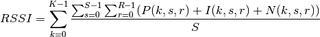
where  is the number of OFDM symbols carrying RS in a RB and
  is the number of REs carrying a RS in a OFDM symbol (which is fixed to
  ) while
  ,
,  and
and  represent respectively the perceived power of the serving cell, the interference power and the noise power of the RE in symbol
  . As for RSRP, the measurements within a RB are always equals among each others according to the PHY model; therefore
  ,
,  and
and  , which implies that the RSSI can be calculated as:

Considering the constraints of the PHY reception chain implementation, and in order to maintain the level of computational complexity low, only RSRP can be directly obtained for all the cells. This is due to the fact that LteSpectrumPhy is designed for evaluating the interference only respect to the signal of the serving eNB. This implies that the PHY layer is optimized for managing the power signals information with the serving eNB as a reference. However, RSRP and RSRQ of neighbor cell can be extracted by the current information available of the serving cell  as detailed in the following:
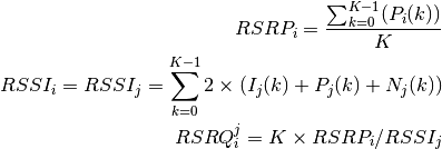
where  is the RSRP of the neighbor cell ,
  is the power perceived at any RE within the RB , is the total number of RBs,
  is the RSSI of the neighbor cell when the UE is attached to cell (which, since it is the sum of all the received powers, coincides with
  ),
),  is the total interference perceived by UE in any RE of RB when attached to cell (obtained by the
 LteInterferencePowerChunkProcessor),  is the power perceived of cell in any RE of the RB and
  is the power noise spectral density in any RE. The sample is considered as valid in case of the RSRQ evaluated is above the
 LteUePhy::RsrqUeMeasThreshold attribute.
HARQ
The HARQ scheme implemented is based on a incremental redundancy (IR) solutions combined with multiple stop-and-wait processes for enabling a continuous data flow. In detail, the solution adopted is the soft combining hybrid IR Full incremental redundancy (also called IR Type II), which implies that the retransmissions contain only new information respect to the previous ones. The resource allocation algorithm of the HARQ has been implemented within the respective scheduler classes (i.e., RrFfMacScheduler and PfFfMacScheduler, refer to their correspondent sections for more info), while the decodification part of the HARQ has been implemented in the LteSpectrumPhy and LteHarqPhy classes which will be detailed in this section.
According to the standard, the UL retransmissions are synchronous and therefore are allocated 7 ms after the original transmission. On the other hand, for the DL, they are asynchronous and therefore can be allocated in a more flexible way starting from 7 ms and it is a matter of the specific scheduler implementation. The HARQ processes behavior is depicted in Figure:ref:fig-harq-processes-scheme.
At the MAC layer, the HARQ entity residing in the scheduler is in charge of controlling the 8 HARQ processes for generating new packets and managing the retransmissions both for the DL and the UL. The scheduler collects the HARQ feedback from eNB and UE PHY layers (respectively for UL and DL connection) by means of the FF API primitives SchedUlTriggerReq and SchedUlTriggerReq. According to the HARQ feedback and the RLC buffers status, the scheduler generates a set of DCIs including both retransmissions of HARQ blocks received erroneous and new transmissions, in general, giving priority to the former. On this matter, the scheduler has to take into consideration one constraint when allocating the resource for HARQ retransmissions, it must use the same modulation order of the first transmission attempt (i.e., QPSK for MCS ![\in [0..9]](_images/math/1849fb6b73087f05f61f9727b9787943adb71597.png) , 16QAM for MCS
, 16QAM for MCS ![\in [10..16]](_images/math/1154dc91a8376df6868a0f74df2bfcc20424697d.png) and 64QAM for MCS
and 64QAM for MCS ![\in [17..28]](_images/math/a7edfe011c65458a26d9d1488f23d2c805663f4e.png) ). This restriction comes from the specification of the rate matcher in the 3GPP standard [
TS36212]_, where the algorithm fixes the modulation order for generating the different blocks of the redundancy versions.
). This restriction comes from the specification of the rate matcher in the 3GPP standard [
TS36212]_, where the algorithm fixes the modulation order for generating the different blocks of the redundancy versions.
The PHY Error Model model (i.e., the LteMiErrorModel class already presented before) has been extended for considering IR HARQ according to [wimaxEmd], where the parameters for the AWGN curves mapping for MIESM mapping in case of retransmissions are given by:
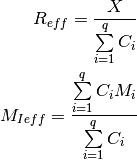
where  is the number of original information bits,
  are number of coded bits,
  are the mutual information per HARQ block received on the total number of
  retransmissions. Therefore, in order to be able to return the error probability with the error model implemented in the simulator evaluates the
  and the
  and return the value of error probability of the ECR of the same modulation with closest lower rate respect to the . In order to consider the effect of HARQ retransmissions a new sets of curves have been integrated respect to the standard one used for the original MCS. The new curves are intended for covering the cases when the most conservative MCS of a modulation is used which implies the generation of lower respect to the one of standard MCSs. On this matter the curves for 1, 2 and 3 retransmissions have been evaluated for 10 and 17. For MCS 0 we considered only the first retransmission since the
produced code rate is already very conservative (i.e., 0.04) and returns an error rate enough robust for the reception (i.e., the downturn of the BLER is centered around -18 dB).
It is to be noted that, the size of first TB transmission has been assumed as containing all the information bits to be coded; therefore is equal to the size of the first TB sent of a an HARQ process. The model assumes that the eventual presence of parity bits in the codewords is already considered in the link level curves. This implies that as soon as the minimum is reached the model is not including the gain due to the transmission of further parity bits.
and return the value of error probability of the ECR of the same modulation with closest lower rate respect to the . In order to consider the effect of HARQ retransmissions a new sets of curves have been integrated respect to the standard one used for the original MCS. The new curves are intended for covering the cases when the most conservative MCS of a modulation is used which implies the generation of lower respect to the one of standard MCSs. On this matter the curves for 1, 2 and 3 retransmissions have been evaluated for 10 and 17. For MCS 0 we considered only the first retransmission since the
produced code rate is already very conservative (i.e., 0.04) and returns an error rate enough robust for the reception (i.e., the downturn of the BLER is centered around -18 dB).
It is to be noted that, the size of first TB transmission has been assumed as containing all the information bits to be coded; therefore is equal to the size of the first TB sent of a an HARQ process. The model assumes that the eventual presence of parity bits in the codewords is already considered in the link level curves. This implies that as soon as the minimum is reached the model is not including the gain due to the transmission of further parity bits.
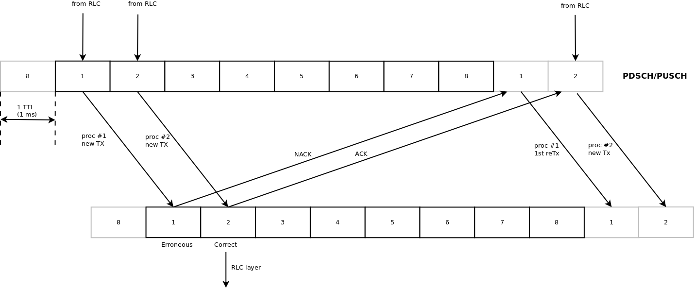
HARQ processes behavior in LTE
The part of HARQ devoted to manage the decodification of the HARQ blocks has been implemented in the LteHarqPhy and LteSpectrumPhy classes. The former is in charge of maintaining the HARQ information for each active process . The latter interacts with LteMiErrorModel class for evaluating the correctness of the blocks received and includes the messaging algorithm in charge of communicating to the HARQ entity in the scheduler the result of the decodifications. These messages are encapsulated in the dlInfoListElement for DL and ulInfoListElement for UL and sent through the PUCCH and the PHICH respectively with an ideal error free model according to the assumptions in their implementation. A sketch of the iteration between HARQ and LTE protocol stack in represented in Figure:ref:fig-harq-architecture.
Finally, the HARQ engine is always active both at MAC and PHY layer; however, in case of the scheduler does not support HARQ the system will continue to work with the HARQ functions inhibited (i.e., buffers are filled but not used). This implementation characteristic gives backward compatibility with schedulers implemented before HARQ integration.
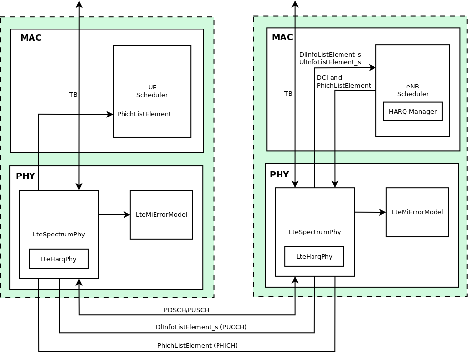
Interaction between HARQ and LTE protocol stack
MAC
Resource Allocation Model
We now briefly describe how resource allocation is handled in LTE, clarifying how it is modeled in the simulator. The scheduler is in charge of generating specific structures called Data Control Indication (DCI) which are then transmitted by the PHY of the eNB to the connected UEs, in order to inform them of the resource allocation on a per subframe basis. In doing this in the downlink direction, the scheduler has to fill some specific fields of the DCI structure with all the information, such as: the Modulation and Coding Scheme (MCS) to be used, the MAC Transport Block (TB) size, and the allocation bitmap which identifies which RBs will contain the data transmitted by the eNB to each user.
For the mapping of resources to physical RBs, we adopt a localized mapping approach (see [Sesia2009], Section 9.2.2.1); hence in a given subframe each RB is always allocated to the same user in both slots. The allocation bitmap can be coded in different formats; in this implementation, we considered the Allocation Type 0 defined in [TS36213], according to which the RBs are grouped in Resource Block Groups (RBG) of different size determined as a function of the Transmission Bandwidth Configuration in use.
For certain bandwidth values not all the RBs are usable, since the group size is not a common divisor of the group. This is for instance the case when the bandwidth is equal to 25 RBs, which results in a RBG size of 2 RBs, and therefore 1 RB will result not addressable. In uplink the format of the DCIs is different, since only adjacent RBs can be used because of the SC-FDMA modulation. As a consequence, all RBs can be allocated by the eNB regardless of the bandwidth configuration.
Adaptive Modulation and Coding
The simulator provides two Adaptive Modulation and Coding (AMC) models: one based on the GSoC model [Piro2011] and one based on the physical error model (described in the following sections).
The former model is a modified version of the model described in [Piro2011],
which in turn is inspired from [Seo2004]. Our version is described in the
following. Let denote the
generic user, and let  be its SINR. We get the spectral efficiency
 of user using the following equations:
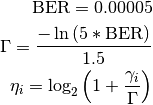
The procedure described in [R1-081483] is used to get the corresponding MCS scheme. The spectral efficiency is quantized based on the channel quality indicator (CQI), rounding to the lowest value, and is mapped to the corresponding MCS scheme.
Finally, we note that there are some discrepancies between the MCS index in [R1-081483] and that indicated by the standard: [TS36213] Table 7.1.7.1-1 says that the MCS index goes from 0 to 31, and 0 appears to be a valid MCS scheme (TB size is not 0) but in [R1-081483] the first useful MCS index is 1. Hence to get the value as intended by the standard we need to subtract 1 from the index reported in [R1-081483].
The alternative model is based on the physical error model developed for this simulator and explained in the following subsections. This scheme is able to adapt the MCS selection to the actual PHY layer performance according to the specific CQI report. According to their definition, a CQI index is assigned when a single PDSCH TB with the modulation coding scheme and code rate correspondent to that CQI index in table 7.2.3-1 of [TS36213] can be received with an error probability less than 0.1. In case of wideband CQIs, the reference TB includes all the RBGs available in order to have a reference based on the whole available resources; while, for subband CQIs, the reference TB is sized as the RBGs.
Transport Block model
The model of the MAC Transport Blocks (TBs) provided by the simulator is simplified with respect to the 3GPP specifications. In particular, a simulator-specific class (PacketBurst) is used to aggregate MAC SDUs in order to achieve the simulator’s equivalent of a TB, without the corresponding implementation complexity. The multiplexing of different logical channels to and from the RLC layer is performed using a dedicated packet tag (LteRadioBearerTag), which performs a functionality which is partially equivalent to that of the MAC headers specified by 3GPP.
The FemtoForum MAC Scheduler Interface
This section describes the ns-3 specific version of the LTE MAC Scheduler Interface Specification published by the FemtoForum [FFAPI].
We implemented the ns-3 specific version of the FemtoForum MAC Scheduler Interface [FFAPI] as a set of C++ abstract classes; in particular, each primitive is translated to a C++ method of a given class. The term implemented here is used with the same meaning adopted in [FFAPI], and hence refers to the process of translating the logical interface specification to a particular programming language. The primitives in [FFAPI] are grouped in two groups: the CSCHED primitives, which deal with scheduler configuration, and the SCHED primitives, which deal with the execution of the scheduler. Furthermore, [FFAPI] defines primitives of two different kinds: those of type REQ go from the MAC to the Scheduler, and those of type IND/CNF go from the scheduler to the MAC. To translate these characteristics into C++, we define the following abstract classes that implement Service Access Points (SAPs) to be used to issue the primitives:
- the
FfMacSchedSapProviderclass defines all the C++ methods that correspond to SCHED primitives of type REQ;- the
FfMacSchedSapUserclass defines all the C++ methods that correspond to SCHED primitives of type CNF/IND;- the
FfMacCschedSapProviderclass defines all the C++ methods that correspond to CSCHED primitives of type REQ;- the
FfMacCschedSapUserclass defines all the C++ methods that correspond to CSCHED primitives of type CNF/IND;
There are 3 blocks involved in the MAC Scheduler interface: Control block, Subframe block and Scheduler block. Each of these blocks provide one part of the MAC Scheduler interface. The figure below shows the relationship between the blocks and the SAPs defined in our implementation of the MAC Scheduler Interface.
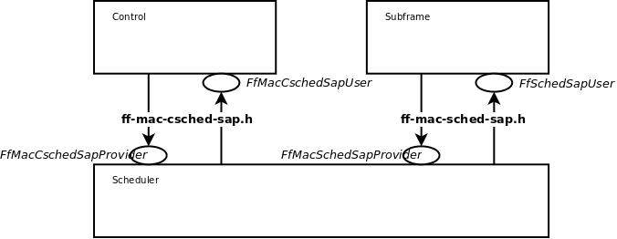
In addition to the above principles, the following design choices have been taken:
- The definition of the MAC Scheduler interface classes follows the naming conventions of the ns-3 Coding Style. In particular, we follow the CamelCase convention for the primitive names. For example, the primitive
CSCHED_CELL_CONFIG_REQis translated toCschedCellConfigReqin the ns-3 code.- The same naming conventions are followed for the primitive parameters. As the primitive parameters are member variables of classes, they are also prefixed with a
m_.- regarding the use of vectors and lists in data structures, we note that [FFAPI] is a pretty much C-oriented API. However, considered that C++ is used in ns-3, and that the use of C arrays is discouraged, we used STL vectors (
std::vector) for the implementation of the MAC Scheduler Interface, instead of using C arrays as implicitly suggested by the way [FFAPI] is written.- In C++, members with constructors and destructors are not allow in
unions. Hence all those data structures that are said to beunionsin [FFAPI] have been defined asstructsin our code.
The figure below shows how the MAC Scheduler Interface is used within the eNB.
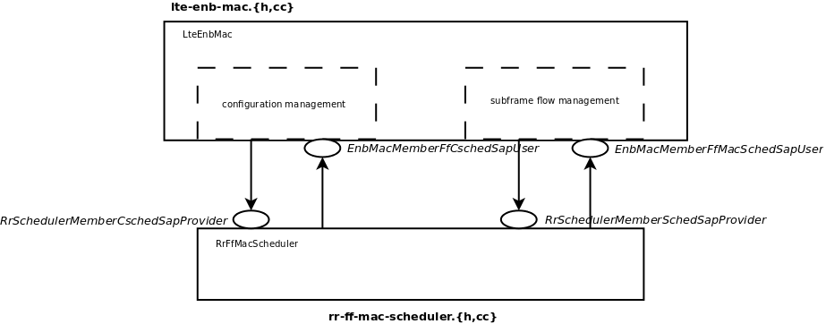
The User side of both the CSCHED SAP and the SCHED SAP are
implemented within the eNB MAC, i.e., in the file lte-enb-mac.cc.
The eNB MAC can be used with different scheduler implementations without
modifications. The same figure also shows, as an example, how the Round Robin
Scheduler is implemented: to interact with the MAC of the eNB, the Round Robin
scheduler implements the Provider side of the SCHED SAP and CSCHED
SAP interfaces. A similar approach can be used to implement other schedulers as
well. A description of each of the scheduler implementations that we provide as
part of our LTE simulation module is provided in the following subsections.
Round Robin (RR) Scheduler
The Round Robin (RR) scheduler is probably the simplest scheduler found in the literature. It works by dividing the available resources among the active flows, i.e., those logical channels which have a non-empty RLC queue. If the number of RBGs is greater than the number of active flows, all the flows can be allocated in the same subframe. Otherwise, if the number of active flows is greater than the number of RBGs, not all the flows can be scheduled in a given subframe; then, in the next subframe the allocation will start from the last flow that was not allocated. The MCS to be adopted for each user is done according to the received wideband CQIs.
For what concern the HARQ, RR implements the non adaptive version, which implies that in allocating the retransmission attempts RR uses the same allocation configuration of the original block, which means maintaining the same RBGs and MCS. UEs that are allocated for HARQ retransmissions are not considered for the transmission of new data in case they have a transmission opportunity available in the same TTI. Finally, HARQ can be disabled with ns3 attribute system for maintaining backward compatibility with old test cases and code, in detail:
Config::SetDefault ("ns3::RrFfMacScheduler::HarqEnabled", BooleanValue (false));
The scheduler implements the filtering of the uplink CQIs according to their nature with UlCqiFilter attribute, in detail:
SRS_UL_CQI: only SRS based CQI are stored in the internal attributes.PUSCH_UL_CQI: only PUSCH based CQI are stored in the internal attributes.
Proportional Fair (PF) Scheduler
The Proportional Fair (PF) scheduler [Sesia2009] works by scheduling a user
when its
instantaneous channel quality is high relative to its own average channel
condition over time. Let  denote generic users; let
  be the
subframe index, and be the resource block index; let
be the
subframe index, and be the resource block index; let  be MCS
usable by user on resource block according to what reported by the AMC
model (see Adaptive Modulation and Coding); finally, let
be MCS
usable by user on resource block according to what reported by the AMC
model (see Adaptive Modulation and Coding); finally, let  be the TB
size in bits as defined in [TS36213] for the case where a number of
resource blocks is used. The achievable rate
be the TB
size in bits as defined in [TS36213] for the case where a number of
resource blocks is used. The achievable rate  in bit/s for user
on resource block group at subframe is defined as
in bit/s for user
on resource block group at subframe is defined as
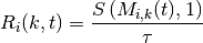
where  is the TTI duration.
At the start of each subframe , each RBG is assigned to a certain user.
In detail, the index
is the TTI duration.
At the start of each subframe , each RBG is assigned to a certain user.
In detail, the index  to which RBG is assigned at time
is determined as
to which RBG is assigned at time
is determined as
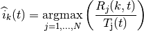
where  is the past througput performance perceived by the
user .
According to the above scheduling algorithm, a user can be allocated to
different RBGs, which can be either adjacent or not, depending on the current
condition of the channel and the past throughput performance . The
latter is determined at the end of the subframe using the following
exponential moving average approach:
is the past througput performance perceived by the
user .
According to the above scheduling algorithm, a user can be allocated to
different RBGs, which can be either adjacent or not, depending on the current
condition of the channel and the past throughput performance . The
latter is determined at the end of the subframe using the following
exponential moving average approach:
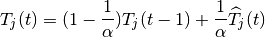
where is the time constant (in number of subframes) of
the exponential moving average, and  is the actual
throughput achieved by the user in the subframe .
is measured according to the following procedure. First we
determine the MCS
is the actual
throughput achieved by the user in the subframe .
is measured according to the following procedure. First we
determine the MCS  actually used by user
:
actually used by user
:
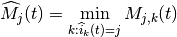
then we determine the total number  of RBGs allocated to user
:
of RBGs allocated to user
:
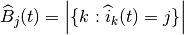
where  indicates the cardinality of the set; finally,
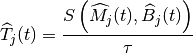
For what concern the HARQ, PF implements the non adaptive version, which implies that in allocating the retransmission attempts the scheduler uses the same allocation configuration of the original block, which means maintaining the same RBGs and MCS. UEs that are allocated for HARQ retransmissions are not considered for the transmission of new data in case they have a transmission opportunity available in the same TTI. Finally, HARQ can be disabled with ns3 attribute system for maintaining backward compatibility with old test cases and code, in detail:
Config::SetDefault ("ns3::PfFfMacScheduler::HarqEnabled", BooleanValue (false));
Maximum Throughput (MT) Scheduler
The Maximum Throughput (MT) scheduler [FCapo2012] aims to maximize the overall throughput of eNB.
It allocates each RB to the user that can achieve the maximum achievable rate in the current TTI.
Currently, MT scheduler in NS-3 has two versions: frequency domain (FDMT) and time domain (TDMT).
In FDMT, every TTI, MAC scheduler allocates RBGs to the UE who has highest achievable rate calculated
by subband CQI. In TDMT, every TTI, MAC scheduler selects one UE which has highest achievable rate
calculated by wideband CQI. Then MAC scheduler allocates all RBGs to this UE in current TTI.
The calculation of achievable rate in FDMT and TDMT is as same as the one in PF.
Let denote generic users; let be the
subframe index, and be the resource block index; let be MCS
usable by user on resource block according to what reported by the AMC
model (see Adaptive Modulation and Coding); finally, let be the TB
size in bits as defined in [TS36213] for the case where a number of
resource blocks is used. The achievable rate in bit/s for user
on resource block at subframe is defined as
where is the TTI duration.
At the start of each subframe , each RB is assigned to a certain user.
In detail, the index to which RB is assigned at time
is determined as

When there are several UEs having the same achievable rate, current implementation always selects the first UE created in script. Although MT can maximize cell throughput, it cannot provide fairness to UEs in poor channel condition.
Throughput to Average (TTA) Scheduler
The Throughput to Average (TTA) scheduler [FCapo2012] can be considered as an intermediate between MT and PF. The metric used in TTA is calculated as follows:
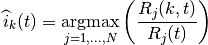
Here, in bit/s represents the achievable rate for user
on resource block at subframe . The
calculation method already is shown in MT and PF. Meanwhile,  in bit/s stands
for the achievable rate for at subframe . The difference between those two
achievable rates is how to get MCS. For , MCS is calculated by subband CQI while
is calculated by wideband CQI. TTA scheduler can only be implemented in frequency domain (FD) because
the achievable rate of particular RBG is only related to FD scheduling.
in bit/s stands
for the achievable rate for at subframe . The difference between those two
achievable rates is how to get MCS. For , MCS is calculated by subband CQI while
is calculated by wideband CQI. TTA scheduler can only be implemented in frequency domain (FD) because
the achievable rate of particular RBG is only related to FD scheduling.
Blind Average Throughput Scheduler
The Blind Average Throughput scheduler [FCapo2012] aims to provide equal throughput to all UEs under eNB. The metric used in TTA is calculated as follows:
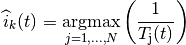
where is the past throughput performance perceived by the user and can be calculated by the
same method in PF scheduler. In the time domain blind average throughput (TD-BET), the scheduler selects the UE
with largest priority metric and allocates all RBGs to this UE. On the other hand, in the frequency domain blind
average throughput (FD-BET), every TTI, the scheduler first selects one UE with lowest pastAverageThroughput (largest
priority metric). Then scheduler assigns one RBG to this UE, it calculates expected throughput of this UE and uses it
to compare with past average throughput of other UEs. The scheduler continues
to allocate RBG to this UE until its expected throughput is not the smallest one among past average throughput
of all UE. Then the scheduler will use the same way to allocate RBG for a new UE which has the
lowest past average throughput until all RBGs are allocated to UEs. The principle behind this is
that, in every TTI, the scheduler tries the best to achieve the equal throughput among all UEs.
Token Bank Fair Queue Scheduler
Token Bank Fair Queue (TBFQ) is a QoS aware scheduler which derives from the leaky-bucket mechanism. In TBFQ,
a traffic flow of user is characterized by following parameters:
: packet arrival rate (byte/sec )
: token generation rate (byte/sec)
: token pool size (byte)
: counter that records the number of token borrowed from or given to the token bank by flow
Each K bytes data consumes k tokens. Also, TBFQ maintains a shared token bank () so as to balance the traffic
between different flows. If token generation rate is bigger than packet arrival rate , then tokens
overflowing from token pool are added to the token bank, and is increased by the same amount. Otherwise,
flow needs to withdraw tokens from token bank based on a priority metric  , and is decreased.
Obviously, the user contributes more on token bank has higher priority to borrow tokens; on the other hand, the
user borrows more tokens from bank has lower priority to continue to withdraw tokens. Therefore, in case of several
users having the same token generation rate, traffic rate and token pool size, user suffers from higher interference
has more opportunity to borrow tokens from bank. In addition, TBFQ can police the traffic by setting the token
generation rate to limit the throughput. Additionally, TBFQ also maintains following three parameters for each flow:
, and is decreased.
Obviously, the user contributes more on token bank has higher priority to borrow tokens; on the other hand, the
user borrows more tokens from bank has lower priority to continue to withdraw tokens. Therefore, in case of several
users having the same token generation rate, traffic rate and token pool size, user suffers from higher interference
has more opportunity to borrow tokens from bank. In addition, TBFQ can police the traffic by setting the token
generation rate to limit the throughput. Additionally, TBFQ also maintains following three parameters for each flow:
- Debt limit
: if
- Credit limit
: the maximum number of tokens UE i can borrow from the bank in one time.
- Credit threshold
: once
LTE in NS-3 has two versions of TBFQ scheduler: frequency domain TBFQ (FD-TBFQ) and time domain TBFQ (TD-TBFQ). In FD-TBFQ, the scheduler always select UE with highest metric and allocates RBG with highest subband CQI until there are no packets within UE’s RLC buffer or all RBGs are allocated [FABokhari2009]. In TD-TBFQ, after selecting UE with maximum metric, it allocates all RBGs to this UE by using wideband CQI [WKWong2004].
Priority Set Scheduler
Priority set scheduler (PSS) is a QoS aware scheduler which combines time domain (TD) and frequency domain (FD) packet scheduling operations into one scheduler [GMonghal2008]. It controls the fairness among UEs by a specified Target Bit Rate (TBR).
In TD scheduler part, PSS first selects UEs with non-empty RLC buffer and then divide them into two sets based on the TBR:
- set 1: UE whose past average throughput is smaller than TBR; TD scheduler calculates their priority metric in Blind Equal Throughput (BET) style:
- set 2: UE whose past average throughput is larger (or equal) than TBR; TD scheduler calculates their priority metric in Proportional Fair (PF) style:
UEs belonged to set 1 have higher priority than ones in set 2. Then PSS will select  UEs with
highest metric in two sets and forward those UE to FD scheduler. In PSS, FD scheduler allocates RBG k to UE n
that maximums the chosen metric. Two PF schedulers are used in PF scheduler:
UEs with
highest metric in two sets and forward those UE to FD scheduler. In PSS, FD scheduler allocates RBG k to UE n
that maximums the chosen metric. Two PF schedulers are used in PF scheduler:
- Proportional Fair scheduled (PFsch)
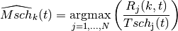
- Carrier over Interference to Average (CoIta)
![\widehat{Mcoi}_{k}(t) = \underset{j=1,...,N}{\operatorname{argmax}}
\left( \frac{ CoI[j,k] }{ \sum_{k=0}^{N_{RBG}} CoI[j,k] } \right)](_images/math/91e089477ab32467b52e5f46a8ee101798aa7077.png)
where  is similar past throughput performance perceived by the user , with the
difference that it is updated only when the i-th user is actually served.
is similar past throughput performance perceived by the user , with the
difference that it is updated only when the i-th user is actually served. ![CoI[j,k]](_images/math/13db3c12c09d8a9234b016015568404b2686bf11.png) is an
estimation of the SINR on the RBG of UE . Both PFsch and CoIta is for decoupling
FD metric from TD scheduler. In addition, PSS FD scheduler also provide a weight metric W[n] for helping
controlling fairness in case of low number of UEs.
is an
estimation of the SINR on the RBG of UE . Both PFsch and CoIta is for decoupling
FD metric from TD scheduler. In addition, PSS FD scheduler also provide a weight metric W[n] for helping
controlling fairness in case of low number of UEs.
![W[n] = max (1, \frac{TBR}{ T_{j}(t) })](_images/math/78cb038b59c380c5dabbd7f29a54229a84db5883.png)
where is the past throughput performance perceived by the user . Therefore, on
RBG k, the FD scheduler selects the UE that maximizes the product of the frequency domain
metric ( ,
,  ) by weight
 ![W[n]](_images/math/0cfa5830cbb0e46a584118fcf423adb4b9115cd3.png) . This strategy will guarantee the throughput of lower
quality UE tend towards the TBR.
. This strategy will guarantee the throughput of lower
quality UE tend towards the TBR.
Config::SetDefault ("ns3::PfFfMacScheduler::HarqEnabled", BooleanValue (false));
The scheduler implements the filtering of the uplink CQIs according to their nature with UlCqiFilter attribute, in detail:
SRS_UL_CQI: only SRS based CQI are stored in the internal attributes.PUSCH_UL_CQI: only PUSCH based CQI are stored in the internal attributes.
Channel and QoS Aware Scheduler
The Channel and QoS Aware (CQA) Scheduler [Bbojovic2014] is an LTE MAC downlink scheduling algorithm that considers the head of line (HOL) delay, the GBR parameters and channel quality over different subbands. The CQA scheduler is based on joint TD and FD scheduling.
In the TD (at each TTI) the CQA scheduler groups users by
priority. The purpose of grouping is to enforce the FD scheduling to
consider first the flows with highest HOL delay. The grouping metric
 for user
  is defined in the
following way:
is defined in the
following way:
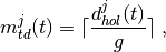
where  is the current value of HOL delay of flow
, and
is the current value of HOL delay of flow
, and  is a grouping parameter that determines
granularity of the groups, i.e. the number of the flows that will be
considered in the FD scheduling iteration.
is a grouping parameter that determines
granularity of the groups, i.e. the number of the flows that will be
considered in the FD scheduling iteration.
The groups of flows selected in the TD iteration are forwarded to the FD
scheduling starting from the flows with the highest value of the
metric until all RBGs are assigned in the corresponding
TTI. In the FD, for each RBG  , the CQA scheduler
assigns the current RBG to the user that has the maximum value of
the FD metric which we define in the following way:
, the CQA scheduler
assigns the current RBG to the user that has the maximum value of
the FD metric which we define in the following way:

where  is calculated as follows:
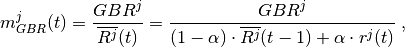
where  is the bit rate specified in EPS bearer of the
flow ,
is the bit rate specified in EPS bearer of the
flow ,  is the past averaged throughput that is calculated with a
moving average,
is the past averaged throughput that is calculated with a
moving average,  is the throughput achieved at the
time t, and is a coefficient such that
is the throughput achieved at the
time t, and is a coefficient such that  .
.
For  we consider two different
metrics:
we consider two different
metrics:  and
and  .
.
 is the Proportional Fair metric which is defined as follows:
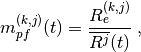
where  is the estimated achievable throughput of user
over RBG calculated by the Adaptive Modulation and Coding
(AMC) scheme that maps the channel quality indicator (CQI) value to
the transport block size in bits.
is the estimated achievable throughput of user
over RBG calculated by the Adaptive Modulation and Coding
(AMC) scheme that maps the channel quality indicator (CQI) value to
the transport block size in bits.
The other channel awareness metric that we consider is  which
is proposed in [GMonghal2008] and it represents the frequency
selective fading gains over RBG for user and is calculated in
the following way:
which
is proposed in [GMonghal2008] and it represents the frequency
selective fading gains over RBG for user and is calculated in
the following way:
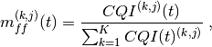
where  is the last reported CQI value from user
for the -th RBG.
is the last reported CQI value from user
for the -th RBG.
The user can select whether or is used
by setting the attribute ns3::CqaFfMacScheduler::CqaMetric
respectively to "CqaPf" or "CqaFf".
Random Access
The LTE model includes a model of the Random Access procedure based on some simplifying assumptions, which are detailed in the following for each of the messages and signals described in the specs [TS36321].
- Random Access (RA) preamble: in real LTE systems this corresponds to a Zadoff-Chu (ZC) sequence using one of several formats available and sent in the PRACH slots which could in principle overlap with PUSCH. PRACH Configuration Index 14 is assumed, i.e., preambles can be sent on any system frame number and subframe number. The RA preamble is modeled using the LteControlMessage class, i.e., as an ideal message that does not consume any radio resources. The collision of preamble transmission by multiple UEs in the same cell are modeled using a protocol interference model, i.e., whenever two or more identical preambles are transmitted in same cell at the same TTI, no one of these identical preambles will be received by the eNB. Other than this collision model, no error model is associated with the reception of a RA preamble.
- Random Access Response (RAR): in real LTE systems, this is a special MAC PDU sent on the DL-SCH. Since MAC control elements are not accurately modeled in the simulator (only RLC and above PDUs are), the RAR is modeled as an LteControlMessage that does not consume any radio resources. Still, during the RA procedure, the LteEnbMac will request to the scheduler the allocation of resources for the RAR using the FF MAC Scheduler primitive SCHED_DL_RACH_INFO_REQ. Hence, an enhanced scheduler implementation (not available at the moment) could allocate radio resources for the RAR, thus modeling the consumption of Radio Resources for the transmission of the RAR.
- Message 3: in real LTE systems, this is an RLC TM SDU sent over resources specified in the UL Grant in the RAR. In the simulator, this is modeled as a real RLC TM RLC PDU whose UL resources are allocated by the scheduler upon call to SCHED_DL_RACH_INFO_REQ.
- Contention Resolution (CR): in real LTE system, the CR phase is needed to address the case where two or more UE sent the same RA preamble in the same TTI, and the eNB was able to detect this preamble in spite of the collision. Since this event does not occur due to the protocol interference model used for the reception of RA preambles, the CR phase is not modeled in the simulator, i.e., the CR MAC CE is never sent by the eNB and the UEs consider the RA to be successful upon reception of the RAR. As a consequence, the radio resources consumed for the transmission of the CR MAC CE are not modeled.
Figure Sequence diagram of the Contention-based MAC Random Access procedure and Sequence diagram of the Non-contention-based MAC Random Access procedure shows the sequence diagrams of respectively the contention-based and non-contention-based MAC random access procedure, highlighting the interactions between the MAC and the other entities.
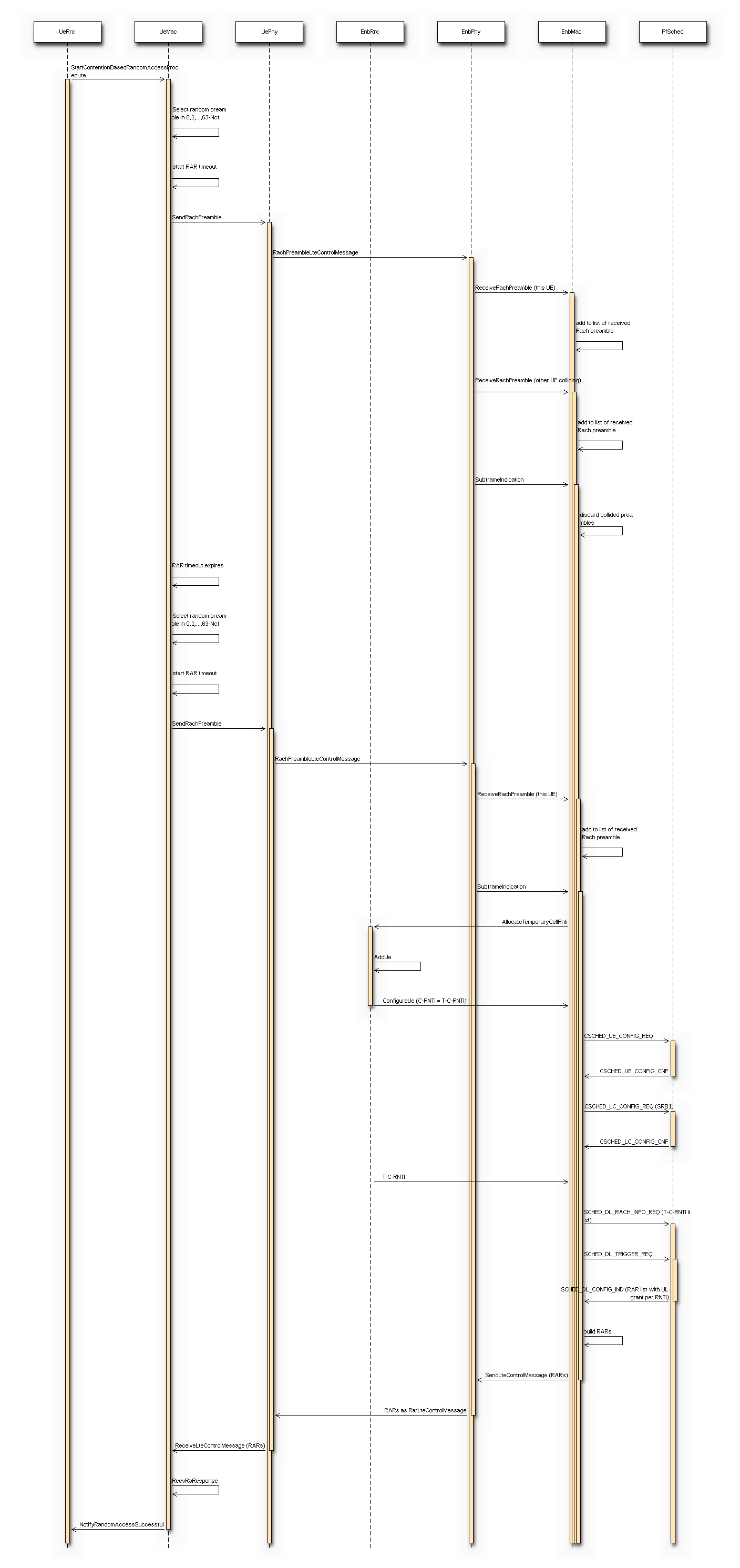
Sequence diagram of the Contention-based MAC Random Access procedure
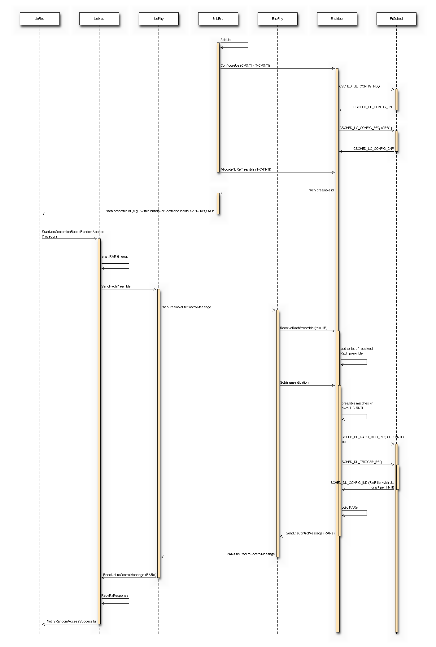
Sequence diagram of the Non-contention-based MAC Random Access procedure
RLC
Overview
The RLC entity is specified in the 3GPP technical specification [TS36322], and comprises three different types of RLC: Transparent Mode (TM), Unacknowledged Mode (UM) and Acknowledged Mode (AM). The simulator includes one model for each of these entities
The RLC entities provide the RLC service interface to the upper PDCP layer and the MAC service interface to the lower MAC layer. The RLC entities use the PDCP service interface from the upper PDCP layer and the MAC service interface from the lower MAC layer.
Figure Implementation Model of PDCP, RLC and MAC entities and SAPs shows the implementation model of the RLC entities and its relationship with all the other entities and services in the protocol stack.
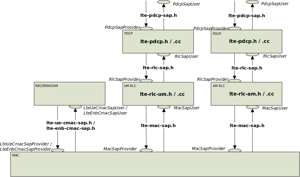
Implementation Model of PDCP, RLC and MAC entities and SAPs
Service Interfaces
RLC Service Interface
The RLC service interface is divided into two parts:
- the
RlcSapProviderpart is provided by the RLC layer and used by the upper PDCP layer and- the
RlcSapUserpart is provided by the upper PDCP layer and used by the RLC layer.
Both the UM and the AM RLC entities provide the same RLC service interface to the upper PDCP layer.
The following list specifies which service primitives are provided by the RLC service interfaces:
RlcSapProvider::TransmitPdcpPdu
- The PDCP entity uses this primitive to send a PDCP PDU to the lower RLC entity in the transmitter peer
RlcSapUser::ReceivePdcpPdu
- The RLC entity uses this primitive to send a PDCP PDU to the upper PDCP entity in the receiver peer
MAC Service Interface
The MAC service interface is divided into two parts:
- the
MacSapProviderpart is provided by the MAC layer and used by the upper RLC layer and- the
MacSapUserpart is provided by the upper RLC layer and used by the MAC layer.
The following list specifies which service primitives are provided by the MAC service interfaces:
MacSapProvider::TransmitPdu
- The RLC entity uses this primitive to send a RLC PDU to the lower MAC entity in the transmitter peer
MacSapProvider::ReportBufferStatus
- The RLC entity uses this primitive to report the MAC entity the size of pending buffers in the transmitter peer
MacSapUser::NotifyTxOpportunity
- The MAC entity uses this primitive to notify the RLC entity a transmission opportunity
MacSapUser::ReceivePdu
- The MAC entity uses this primitive to send an RLC PDU to the upper RLC entity in the receiver peer
AM RLC
The processing of the data transfer in the Acknowledge Mode (AM) RLC entity is explained in section 5.1.3 of [TS36322]. In this section we describe some details of the implementation of the RLC entity.
Buffers for the transmit operations
Our implementation of the AM RLC entity maintains 3 buffers for the transmit operations:
- Transmission Buffer: it is the RLC SDU queue. When the AM RLC entity receives a SDU in the TransmitPdcpPdu service primitive from the upper PDCP entity, it enqueues it in the Transmission Buffer. We put a limit on the RLC buffer size and the LteRlc TxDrop trace source is called when a drop due to a full buffer occurs.
- Transmitted PDUs Buffer: it is the queue of transmitted RLC PDUs for which an ACK/NACK has not been received yet. When the AM RLC entity sends a PDU to the MAC entity, it also puts a copy of the transmitted PDU in the Transmitted PDUs Buffer.
- Retransmission Buffer: it is the queue of RLC PDUs which are considered for retransmission (i.e., they have been NACKed). The AM RLC entity moves this PDU to the Retransmission Buffer, when it retransmits a PDU from the Transmitted Buffer.
Transmit operations in downlink
The following sequence diagram shows the interactions between the different entities (RRC, PDCP, AM RLC, MAC and MAC scheduler) of the eNB in the downlink to perform data communications.
Figure Sequence diagram of data PDU transmission in downlink shows how the upper layers send data PDUs and how the data flow is processed by the different entities/services of the LTE protocol stack.
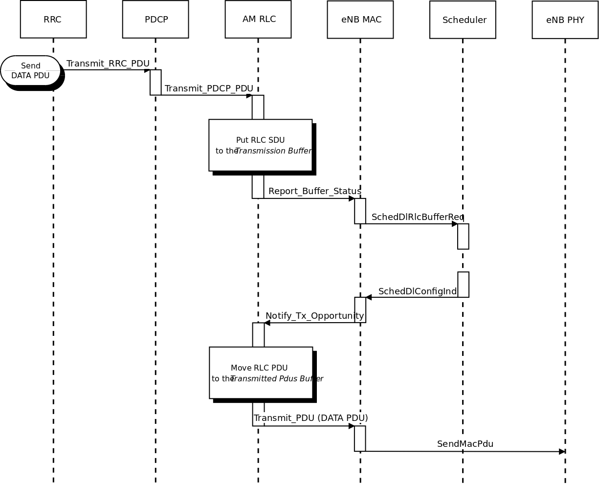
Sequence diagram of data PDU transmission in downlink
The PDCP entity calls the Transmit_PDCP_PDU service primitive in
order to send a data PDU. The AM RLC entity processes this service
primitive according to the AM data transfer procedures defined in
section 5.1.3 of [TS36322].
When the Transmit_PDCP_PDU service primitive is called, the AM RLC
entity performs the following operations:
- Put the data SDU in the Transmission Buffer.
- Compute the size of the buffers (how the size of buffers is computed will be explained afterwards).
- Call the
Report_Buffer_Statusservice primitive of the eNB MAC entity in order to notify to the eNB MAC entity the sizes of the buffers of the AM RLC entity. Then, the eNB MAC entity updates the buffer status in the MAC scheduler using the SchedDlRlcBufferReq service primitive of the FF MAC Scheduler API.
Afterwards, when the MAC scheduler decides that some data can be sent,
the MAC entity notifies it to the RLC entity, i.e. it calls the
Notify_Tx_Opportunity service primitive, then the AM RLC entity
does the following:
- Create a single data PDU by segmenting and/or concatenating the SDUs in the Transmission Buffer.
- Move the data PDU from the Transmission Buffer to the Transmitted PDUs Buffer.
- Update state variables according section 5.1.3.1.1 of [TS36322].
- Call the
Transmit_PDUprimitive in order to send the data PDU to the MAC entity.
Retransmission in downlink
The sequence diagram of Figure Sequence diagram of data PDU retransmission in downlink shows the interactions between the different entities (AM RLC, MAC and MAC scheduler) of the eNB in downlink when data PDUs must be retransmitted by the AM RLC entity.
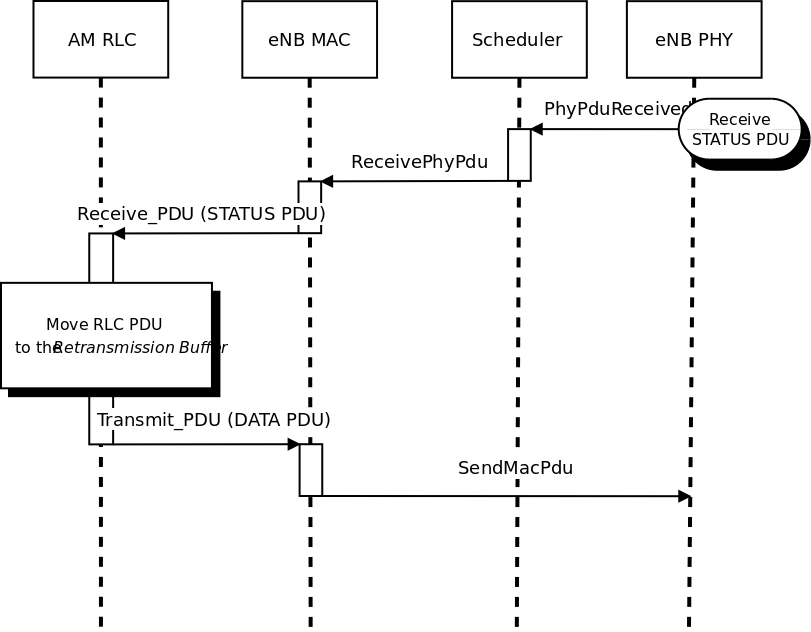
Sequence diagram of data PDU retransmission in downlink
The transmitting AM RLC entity can receive STATUS PDUs from the peer AM RLC entity. STATUS PDUs are sent according section 5.3.2 of [TS36322] and the processing of reception is made according section 5.2.1 of [TS36322].
When a data PDUs is retransmitted from the Transmitted PDUs Buffer, it is also moved to the Retransmission Buffer.
Transmit operations in uplink
The sequence diagram of Figure Sequence diagram of data PDU transmission in uplink shows the interactions between the different entities of the UE (RRC, PDCP, RLC and MAC) and the eNB (MAC and Scheduler) in uplink when data PDUs are sent by the upper layers.
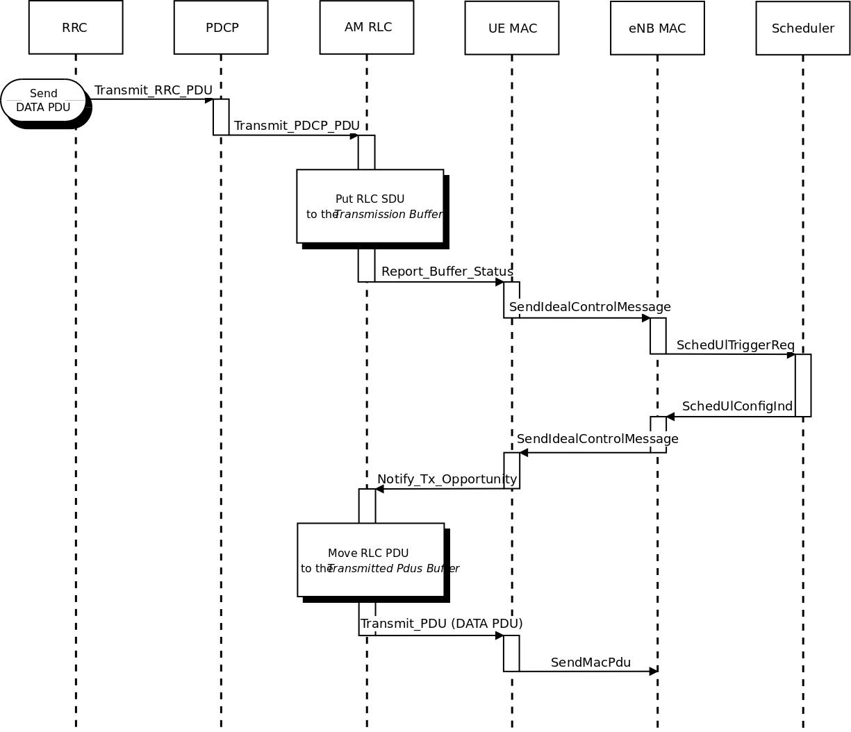
Sequence diagram of data PDU transmission in uplink
It is similar to the sequence diagram in downlink; the main difference is that in this case the Report_Buffer_Status is sent from the UE MAC to the MAC Scheduler in the eNB over the air using the control channel.
Retransmission in uplink
The sequence diagram of Figure Sequence diagram of data PDU retransmission in uplink shows the interactions between the different entities of the UE (AM RLC and MAC) and the eNB (MAC) in uplink when data PDUs must be retransmitted by the AM RLC entity.
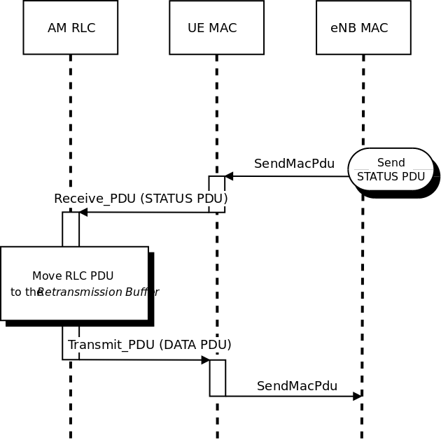
Sequence diagram of data PDU retransmission in uplink
Calculation of the buffer size
The Transmission Buffer contains RLC SDUs. A RLC PDU is one or more SDU segments plus an RLC header. The size of the RLC header of one RLC PDU depends on the number of SDU segments the PDU contains.
The 3GPP standard (section 6.1.3.1 of [TS36321]) says clearly that, for the uplink, the RLC and MAC headers are not considered in the buffer size that is to be report as part of the Buffer Status Report. For the downlink, the behavior is not specified. Neither [FFAPI] specifies how to do it. Our RLC model works by assuming that the calculation of the buffer size in the downlink is done exactly as in the uplink, i.e., not considering the RLC and MAC header size.
We note that this choice affects the interoperation with the
MAC scheduler, since, in response to the
Notify_Tx_Opportunity service primitive, the RLC is expected to
create a PDU of no more than the size requested by the MAC, including
RLC overhead. Hence, unneeded fragmentation can occur if (for example)
the MAC notifies a transmission exactly equal to the buffer size
previously reported by the RLC. We assume that it is left to the Scheduler
to implement smart strategies for the selection of the size of the
transmission opportunity, in order to eventually avoid the inefficiency
of unneeded fragmentation.
Concatenation and Segmentation
The AM RLC entity generates and sends exactly one RLC PDU for each transmission opportunity even if it is smaller than the size reported by the transmission opportunity. So for instance, if a STATUS PDU is to be sent, then only this PDU will be sent in that transmission opportunity.
The segmentation and concatenation for the SDU queue of the AM RLC entity follows the same philosophy as the same procedures of the UM RLC entity but there are new state variables (see [TS36322] section 7.1) only present in the AM RLC entity.
It is noted that, according to the 3GPP specs, there is no concatenation for the Retransmission Buffer.
Re-segmentation
The current model of the AM RLC entity does not support the re-segmentation of the retransmission buffer. Rather, the AM RLC entity just waits to receive a big enough transmission opportunity.
Unsupported features
We do not support the following procedures of [TS36322] :
- “Send an indication of successful delivery of RLC SDU” (See section 5.1.3.1.1)
- “Indicate to upper layers that max retransmission has been reached” (See section 5.2.1)
- “SDU discard procedures” (See section 5.3)
- “Re-establishment procedure” (See section 5.4)
We do not support any of the additional primitives of RLC SAP for AM RLC entity. In particular:
- no SDU discard notified by PDCP
- no notification of successful / failed delivery by AM RLC entity to PDCP entity
UM RLC
In this section we describe the implementation of the Unacknowledged Mode (UM) RLC entity.
Transmit operations in downlink
The transmit operations of the UM RLC are similar to those of the AM RLC previously described in Section Transmit operations in downlink, with the difference that, following the specifications of [TS36322], retransmission are not performed, and there are no STATUS PDUs.
Transmit operations in uplink
The transmit operations in the uplink are similar to those of the downlink, with the main difference that the Report_Buffer_Status is sent from the UE MAC to the MAC Scheduler in the eNB over the air using the control channel.
Calculation of the buffer size
The calculation of the buffer size for the UM RLC is done using the same approach of the AM RLC, please refer to section Calculation of the buffer size for the corresponding description.
TM RLC
In this section we describe the implementation of the Transparent Mode (TM) RLC entity.
Transmit operations in downlink
In the simulator, the TM RLC still provides to the upper layers the same service interface provided by the AM and UM RLC entities to the PDCP layer; in practice, this interface is used by an RRC entity (not a PDCP entity) for the transmission of RLC SDUs. This choice is motivated by the fact that the services provided by the TM RLC to the upper layers, according to [TS36322], is a subset of those provided by the UM and AM RLC entities to the PDCP layer; hence, we reused the same interface for simplicity.
The transmit operations in the downlink are performed as follows. When
the Transmit_PDCP_PDU service primitive is called by the upper
layers, the TM RLC does the following:
- put the SDU in the Transmission Buffer
- compute the size of the Transmission Buffer
- call the
Report_Buffer_Statusservice primitive of the eNB MAC entity
Afterwards, when the MAC scheduler decides that some data can be sent
by the logical channel to which the TM RLC entity belongs, the MAC
entity notifies it to the TM RLC entity by calling the
Notify_Tx_Opportunity service primitive. Upon reception of this
primitive, the TM RLC entity does the following:
- if the TX opportunity has a size that is greater than or equal to the size of the head-of-line SDU in the Transmission Buffer
- dequeue the head-of-line SDU from the Transmission Buffer
- create one RLC PDU that contains entirely that SDU, without any RLC header
- Call the
Transmit_PDUprimitive in order to send the RLC PDU to the MAC entity.
Transmit operations in uplink
The transmit operations in the uplink are similar to those of the downlink, with the main difference that a transmission opportunity can also arise from the assignment of the UL GRANT as part of the Random Access procedure, without an explicit Buffer Status Report issued by the TM RLC entity.
Calculation of the buffer size
As per the specifications [TS36322], the TM RLC does not add any RLC header to the PDUs being transmitted. Because of this, the buffer size reported to the MAC layer is calculated simply by summing the size of all packets in the transmission buffer, thus notifying to the MAC the exact buffer size.
SM RLC
In addition to the AM, UM and TM implementations that are modeled after the 3GPP specifications, a simplified RLC model is provided, which is called Saturation Mode (SM) RLC. This RLC model does not accept PDUs from any above layer (such as PDCP); rather, the SM RLC takes care of the generation of RLC PDUs in response to the notification of transmission opportunities notified by the MAC. In other words, the SM RLC simulates saturation conditions, i.e., it assumes that the RLC buffer is always full and can generate a new PDU whenever notified by the scheduler.
The SM RLC is used for simplified simulation scenarios in which only the LTE Radio model is used, without the EPC and hence without any IP networking support. We note that, although the SM RLC is an unrealistic traffic model, it still allows for the correct simulation of scenarios with multiple flows belonging to different (non real-time) QoS classes, in order to test the QoS performance obtained by different schedulers. This can be done since it is the task of the Scheduler to assign transmission resources based on the characteristics (e.g., Guaranteed Bit Rate) of each Radio Bearer, which are specified upon the definition of each Bearer within the simulation program.
As for schedulers designed to work with real-time QoS traffic that has delay constraints, the SM RLC is probably not an appropriate choice. This is because the absence of actual RLC SDUs (replaced by the artificial generation of Buffer Status Reports) makes it not possible to provide the Scheduler with meaningful head-of-line-delay information, which is often the metric of choice for the implementation of scheduling policies for real-time traffic flows. For the simulation and testing of such schedulers, it is advisable to use either the UM or the AM RLC models instead.
PDCP
PDCP Model Overview
The reference document for the specification of the PDCP entity is [TS36323]. With respect to this specification, the PDCP model implemented in the simulator supports only the following features:
- transfer of data (user plane or control plane);
- maintenance of PDCP SNs;
- transfer of SN status (for use upon handover);
The following features are currently not supported:
- header compression and decompression of IP data flows using the ROHC protocol;
- in-sequence delivery of upper layer PDUs at re-establishment of lower layers;
- duplicate elimination of lower layer SDUs at re-establishment of lower layers for radio bearers mapped on RLC AM;
- ciphering and deciphering of user plane data and control plane data;
- integrity protection and integrity verification of control plane data;
- timer based discard;
- duplicate discarding.
PDCP Service Interface
The PDCP service interface is divided into two parts:
- the
PdcpSapProviderpart is provided by the PDCP layer and used by the upper layer and- the
PdcpSapUserpart is provided by the upper layer and used by the PDCP layer.
PDCP Service Primitives
The following list specifies which service primitives are provided by the PDCP service interfaces:
PdcpSapProvider::TransmitPdcpSdu
- The RRC entity uses this primitive to send an RRC PDU to the lower PDCP entity in the transmitter peer
PdcpSapUser::ReceivePdcpSdu
- The PDCP entity uses this primitive to send an RRC PDU to the upper RRC entity in the receiver peer
RRC
Features
The RRC model implemented in the simulator provides the following functionality:
- generation (at the eNB) and interpretation (at the UE) of System Information (in particular the Master Information Block and, at the time of this writing, only System Information Block Type 1 and 2)
- initial cell selection
- RRC connection establishment procedure
- RRC reconfiguration procedure, supporting the following use cases: + reconfiguration of the SRS configuration index + reconfiguration of the PHY TX mode (MIMO) + reconfiguration of UE measurements + data radio bearer setup + handover
- RRC connection re-establishment, supporting the following use cases: + handover
Architecture
The RRC model is divided into the following components:
- the RRC entities LteUeRrc and LteEnbRrc, which implement the state machines of the RRC entities respectively at the UE and the eNB;
- the RRC SAPs LteUeRrcSapProvider, LteUeRrcSapUser, LteEnbRrcSapProvider, LteEnbRrcSapUser, which allow the RRC entities to send and receive RRC messages and information elmenents;
- the RRC protocol classes LteUeRrcProtocolIdeal, LteEnbRrcProtocolIdeal, LteUeRrcProtocolReal, LteEnbRrcProtocolReal, which implement two different models for the transmission of RRC messages.
Additionally, the RRC components use various other SAPs in order to interact with the rest of the protocol stack. A representation of all the SAPs that are used is provided in the figures LTE radio protocol stack architecture for the UE on the data plane, LTE radio protocol stack architecture for the UE on the control plane, LTE radio protocol stack architecture for the eNB on the data plane and LTE radio protocol stack architecture for the eNB on the control plane.
UE RRC State Machine
In Figure UE RRC State Machine we represent the state machine as implemented in the RRC UE entity.
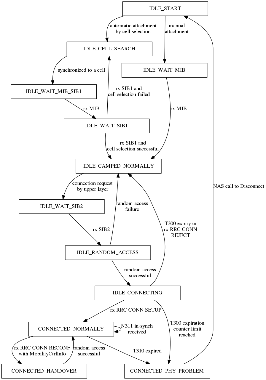
UE RRC State Machine
All the states are transient, however, the UE in “CONNECTED_NORMALLY” state will only switch to the IDLE state if the downlink SINR is below a defined threshold, which would lead to radio link failure Radio Link Failure. One the other hand, the UE would not be able switch to IDLE mode due to a handover failure, as mentioned in X2.
ENB RRC State Machine
The eNB RRC maintains the state for each UE that is attached to the cell. From an implementation point of view, the state of each UE is contained in an instance of the UeManager class. The state machine is represented in Figure ENB RRC State Machine for each UE.

ENB RRC State Machine for each UE
Initial Cell Selection
Initial cell selection is an IDLE mode procedure, performed by UE when it has not yet camped or attached to an eNodeB. The objective of the procedure is to find a suitable cell and attach to it to gain access to the cellular network.
It is typically done at the beginning of simulation, as depicted in Figure Sample runs of initial cell selection in UE and timing of related events below. The time diagram on the left side is illustrating the case where initial cell selection succeed on first try, while the diagram on the right side is for the case where it fails on the first try and succeed on the second try. The timing assumes the use of real RRC protocol model (see RRC protocol models) and no transmission error.
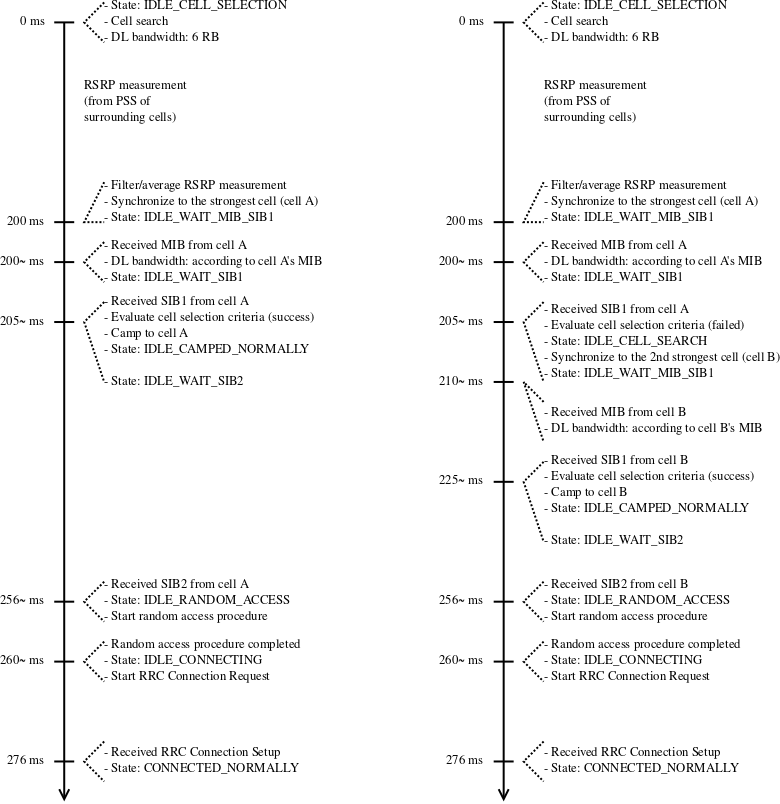
Sample runs of initial cell selection in UE and timing of related events
The functionality is based on 3GPP IDLE mode specifications, such as in [TS36300], [TS36304], and [TS36331]. However, a proper implementation of IDLE mode is still missing in the simulator, so we reserve several simplifying assumptions:
- multiple carrier frequency is not supported;
- multiple Public Land Mobile Network (PLMN) identities (i.e. multiple network operators) is not supported;
- RSRQ measurements are not utilized;
- stored information cell selection is not supported;
- “Any Cell Selection” state and camping to an acceptable cell is not supported;
- marking a cell as barred or reserved is not supported;
- Idle cell reselection is not supported, hence it is not possible for UE to camp to a different cell after the initial camp has been placed; and
- UE’s Closed Subscriber Group (CSG) white list contains only one CSG identity.
Also note that initial cell selection is only available for EPC-enabled simulations. LTE-only simulations must use the manual attachment method. See section Network Attachment of the User Documentation for more information on their differences in usage.
The next subsections cover different parts of initial cell selection, namely cell search, broadcast of system information, and cell selection evaluation.
Cell Search
Cell search aims to detect surrounding cells and measure the strength of received signal from each of these cells. One of these cells will become the UE’s entry point to join the cellular network.
The measurements are based on the RSRP of the received PSS, averaged by Layer 1
filtering, and performed by the PHY layer, as previously described in more
detail in section UE PHY Measurements Model. PSS is transmitted by eNodeB
over the central 72 sub-carriers of the DL channel (Section 5.1.7.3 [TS36300]),
hence we model cell search to operate using a DL bandwidth of 6 RBs. Note that
measurements of RSRQ are not available at this point of time in simulation. As
a consequence, the LteUePhy::RsrqUeMeasThreshold attribute does not apply
during cell search.
By using the measured RSRP, the PHY entity is able to generate a list of detected cells, each with its corresponding cell ID and averaged RSRP. This list is periodically pushed via CPHY SAP to the RRC entity as a measurement report.
The RRC entity inspects the report and simply choose the cell with the strongest RSRP, as also indicated in Section 5.2.3.1 of [TS36304]. Then it instructs back the PHY entity to synchronize to this particular cell. The actual operating bandwidth of the cell is still unknown at this time, so the PHY entity listens only to the minimum bandwidth of 6 RBs. Nevertheless, the PHY entity will be able to receive system broadcast message from this particular eNodeB, which is the topic of the next subsection.
Broadcast of System Information
System information blocks are broadcasted by eNodeB to UEs at predefined time intervals, adapted from Section 5.2.1.2 of [TS36331]. The supported system information blocks are:
- Master Information Block (MIB)
- Contains parameters related to the PHY layer, generated during cell configuration and broadcasted every 10 ms at the beginning of radio frame as a control message.
- System Information Block Type 1 (SIB1)
- Contains information regarding network access, broadcasted every 20 ms at the middle of radio frame as a control message. Not used in manual attachment method. UE must have decoded MIB before it can receive SIB1.
- System Information Block Type 2 (SIB2)
- Contains UL- and RACH-related settings, scheduled to transmit via RRC protocol at 16 ms after cell configuration, and then repeats every 80 ms (configurable through LteEnbRrc::SystemInformationPeriodicity attribute. UE must be camped to a cell in order to be able to receive its SIB2.
Reception of system information is fundamental for UE to advance in its lifecycle. MIB enables the UE to increase the initial DL bandwidth of 6 RBs to the actual operating bandwidth of the network. SIB1 provides information necessary for cell selection evaluation (explained in the next section). And finally SIB2 is required before the UE is allowed to switch to CONNECTED state.
Cell Selection Evaluation
UE RRC reviews the measurement report produced in Cell Search and the cell access information provided by SIB1. Once both information is available for a specific cell, the UE triggers the evaluation process. The purpose of this process is to determine whether the cell is a suitable cell to camp to.
The evaluation process is a slightly simplified version of Section 5.2.3.2 of [TS36304]. It consists of the following criteria:
- Rx level criterion; and
- closed subscriber group (CSG) criterion.
The first criterion, Rx level, is based on the cell’s measured RSRP
 , which has to be higher than a required minimum
 in order to pass the criterion:

where is determined by each eNodeB and is obtainable by UE
from SIB1.
The last criterion, CSG, is a combination of a true-or-false parameter called CSG indication and a simple number CSG identity. The basic rule is that UE shall not camp to eNodeB with a different CSG identity. But this rule is only enforced when CSG indication is valued as true. More details are provided in Section Network Attachment of the User Documentation.
When the cell passes all the above criteria, the cell is deemed as suitable. Then UE camps to it (IDLE_CAMPED_NORMALLY state).
After this, upper layer may request UE to enter CONNECTED mode. Please refer to section RRC connection establishment for details on this.
On the other hand, when the cell does not pass the CSG criterion, then the cell is labeled as acceptable (Section 10.1.1.1 [TS36300]). In this case, the RRC entity will tell the PHY entity to synchronize to the second strongest cell and repeat the initial cell selection procedure using that cell. As long as no suitable cell is found, the UE will repeat these steps while avoiding cells that have been identified as acceptable.
Radio Admission Control
Radio Admission Control is supported by having the eNB RRC
reply to an RRC CONNECTION REQUEST message sent by the UE with either
an RRC CONNECTION SETUP message or an RRC CONNECTION REJECT message,
depending on whether the new UE is to be admitted or not. In the
current implementation, the behavior is determined by the boolean attribute
ns3::LteEnbRrc::AdmitRrcConnectionRequest. There is currently no Radio Admission
Control algorithm that dynamically decides whether a new connection
shall be admitted or not.
Radio Bearer Configuration
Some implementation choices have been made in the RRC regarding the setup of radio bearers:
- three Logical Channel Groups (out of four available) are configured for uplink buffer status report purposes, according to the following policy:
- LCG 0 is for signaling radio bearers
- LCG 1 is for GBR data radio bearers
- LCG 2 is for Non-GBR data radio bearers
Radio Link Failure
In real LTE networks, Radio link failure (RLF) can happen due to several reasons. It can be triggered if a UE is unable to decode PDCCH due to poor signal quality, upon maximum RLC retransmissions, RACH problems and other reasons. 3GPP only specifies guidelines to detect RLF at the UE side, in [TS36331] and [TS36133]. On the other hand, the eNB implementation is expected to be vendor specific. To implement the RLF functionality in ns-3, we have assumed the following simplifications:
- The RLF detection procedure at eNodeB is not implemented. Instead, a direct function call by using the SAP between UE and eNB RRC (for both ideal and real RRC) is used to notify the eNB about the RLF.
- No RRC connection re-establishment procedure is implemented, thus, the UE directly goes to the IDLE state upon RLF. This is in fact as per the standard [TS36331] sec 5.3.11.3, since, at this stage the LTE module does not support the Access Stratum (AS) security.
The above mentioned RLF specifications can be divided into the following two categories:
- RLF detection
- Actions upon RLF detection
In the following, we will explain the RLF implementation in context of these two categories.
RLF detection implementation
The RLF detection at the UE is implemented as per [TS36133], i.e., by monitoring the radio link quality based on the reference signals (which in the simulation is equivalent to the PDCCH) in the downlink. Thus, it is independent of the method used for the downlink CQI computation, i.e., Ctrl method and Mixed method. Moreover, when using FFR, especially for hard-FFR, and CQIs based on Mixed method, UEs might experience relatively good performance and RLF simultaneously. This is due to the fact that the interference in PDSCH is affected by the actual data transmissions on the specific RBs and the power control. Therefore, UEs might experience good SINR in PDSCH, while bad SINR in PDCCH channel. For more details about these methods please refer to CQI feedback. Also, it does not matter if the DL control error model is disabled, a UE can still detect the RLF since the SINR based on the control channel is reported to the LteUePhy class, using a callback hooked in LteHelper while installing a UE device.
The RLF detection starts once the RRC connection is established between UE and
eNodeB, i.e., UE is in “CONNECTED_NORMALLY” state; upon which the RLF parameters
are configured (see LteUePhy::DoConfigureRadioLinkFailureDetection). In real
networks, these parameters are transmitted by the eNB using IE UE-TimersAndConstants or
RLF-TimersAndConstants. However, for the sake of simplification, in the simulator
they are presented as the attributes of the LteUePhy and LteUeRrc classes.
Moreover, what concerns the carrier aggregation, i.e., when a UE is configured
with multiple component carriers, the RLF detection is only performed by the
primary component carrier, i.e. component carrier id 0
(see LteUePhy::DoNotifyConnectionSuccessful). In LteUePhy class, CQI
calculation is triggered for every downlink subframe received,
and the average SINR value is measured across all resource blocks. For the RLF
detection, these SINR values are averaged over a downlink frame and if the result
is less than a defined threshold Qout (default: -5dB), the frame cannot be decoded
(see``LteUePhy::RadioLinkFailureDetection``). The Qout threshold corresponds to 10%
block error rate (BLER) of a hypothetical PDCCH transmission taking into account
the PCFICH errors [R4-081920] (also refer to
Control Channels PHY Error Model). Once, the UE is unable to decode
20 consecutive frames, i.e., the Qout evaluation period (200ms) is reached, an
out-of-sync indication is sent to the UE RRC layer (see LteUeRrc::DoNotifyOutOfSync).
Else, the counter for the unsuccessfully decoded frames is reset to zero. At the
LteUeRrc, when the number of consecutive out-of-sync indications matches with the
value of N310 parameter, the T310 timer is started and LteUePhy is notified to start
measuring for in-sync indications (see LteUePhy::DoStartInSnycDetection). We note
that, the UE RRC state is not changed till the expiration of T310 timer. If the
resultant SINR values averaged over a downlink frame is greater than a defined
threshold Qin (default: -3.8dB), the frame is considered to be successfully
decoded. Qin corresponds to 2% BLER [R4-081920] of a hypothetical PDCCH transmission
taking into account the PCFICH errors. Once the UE is able to decode 10
consecutive frames, an in-sync indication is sent to the UE RRC layer
(see LteUeRrc::DoNotifyInSync). Else, the counter for the successfully decoded
frames is reset to zero. If prior to the T310 timer expiry, the number of
consecutive in-sync indications matches with N311 parameter of LteUeRRC, the UE
is considered back in-sync. At this stage, the related parameters are reset to
initiate the radio link failure detection from the beginning
(see LteUePhy::DoConfigureRadioLinkFailureDetection). On the other hand, If the
T310 timer expires, the UE considers that a RLF has occurred
(see LteUeRrc::RadioLinkFailureDetected).
Actions upon RLF
Once the T310 timer is expired, a UE is considered to be in RLF; upon which the UE RRC:
- Sends a request to the eNB RRC to remove the UE context
- Moves to “CONNECTED_PHY_PROBLEM” state
- Notifies the UE NAS layer about the release of RRC connection.
Then, after getting the notification from the UE RRC the NAS does the following:
- Delete all the TFTs
- Reset the bearer counter
- Restore the bearer list, which is used to activate the bearers for the next RRC connection. This restoration of the bearers is achieved by maintaining an additional list, i.e., m_bearersToBeActivatedListForReconnection in EpcUeNas class
- Switch the NAS state to OFF by calling EpcUeNas::Disconnect
- Tells the UE RRC to disconnect
The UE RRC, upon receiving the call to disconnect from the EpcUeNas class, performs the action as specified by [TS36331] 5.3.11.3, and finally leaves the connected state, i.e., its RRC state is changed from “CONNECTED_PHY_PROBLEM” to “IDLE_START” to perform cell selection as shown in figures UE RRC State Machine and UE procedures after radio link failure.
At this stage, the LTE module does not support the paging functionality, therefore,
to allow a UE to read SIB2 message after camping on a suitable cell after RLF, a
work around is used in LteUeRrc::EvaluateCellForSelection method. As per this
workaround, the UE RRC invokes the call to LteUeRrc::DoConnect method, which
enables the UE to switch its state from “IDLE_CAMPED_NORMALLY” to “IDLE_WAIT_SIB2”,
thus, allowing it to perform the random access.
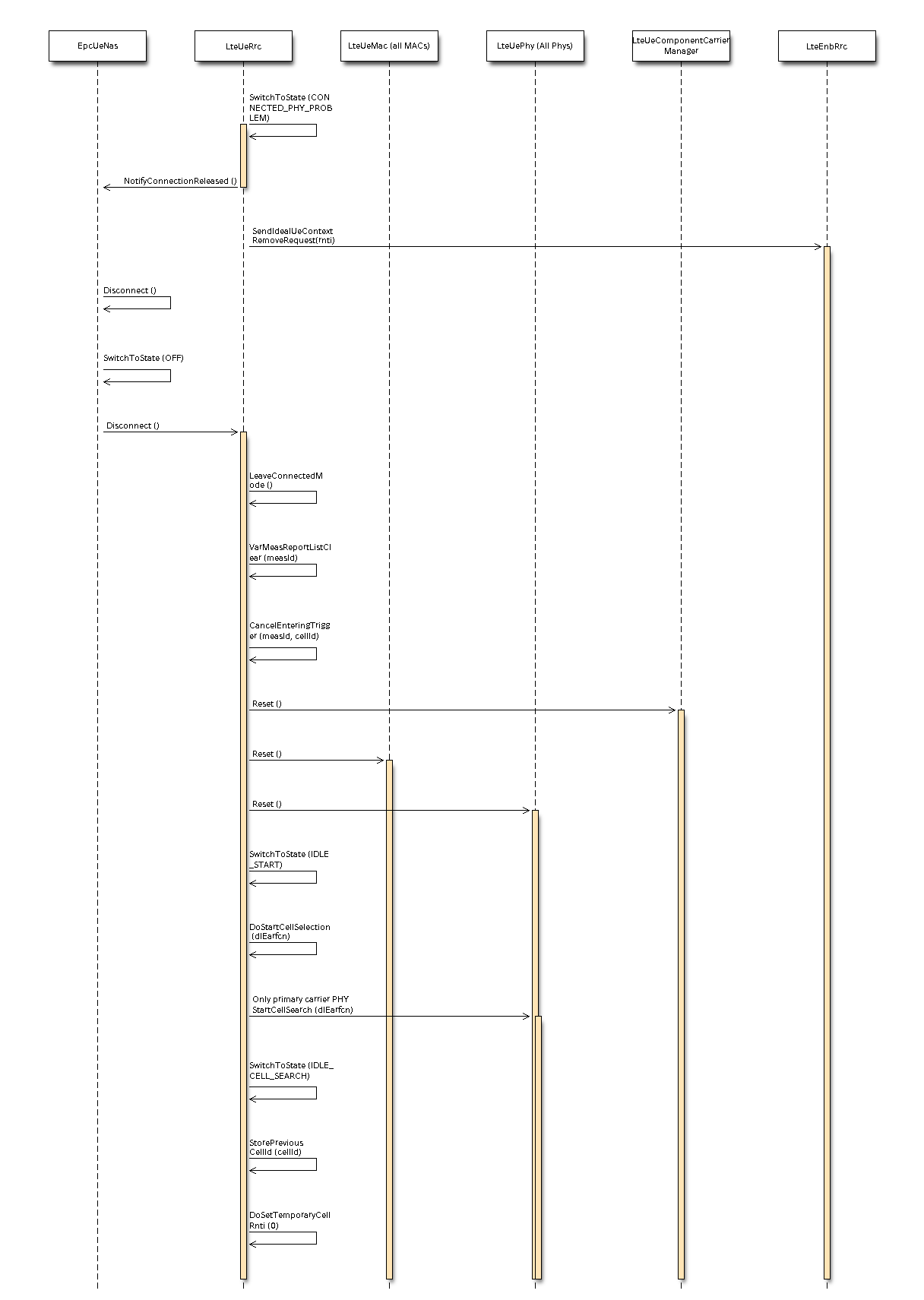
UE procedures after radio link failure
The eNB RRC, after receiving the notification from the UE RRC starts the procedure of UE context deletion, which also involves the deletion of the UE context removal from the EPC UE context removal from EPC and the eNB stack UE context removal from eNB stack. We note that, the UE context at the MME is not removed since, bearers are only added at the start of a simulation in MME, and cannot be added again unless scheduled for addition during a simulation.
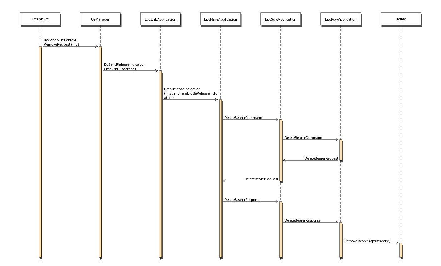
UE context removal from EPC
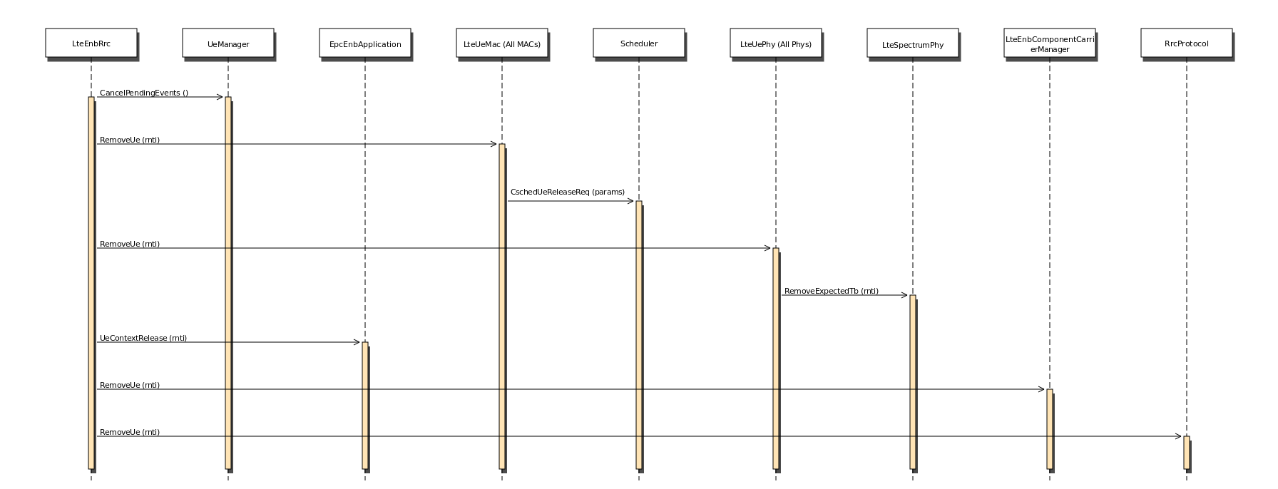
UE context removal from eNB stack
UE RRC Measurements Model
UE RRC measurements support
The UE RRC entity provides support for UE measurements; in particular, it implements the procedures described in Section 5.5 of [TS36331], with the following simplifying assumptions:
- only E-UTRA intra-frequency measurements are supported, which implies:
- only one measurement object is used during the simulation;
- measurement gaps are not needed to perform the measurements;
- Event B1 and B2 are not implemented;
- only reportStrongestCells purpose is supported, while reportCGI and reportStrongestCellsForSON purposes are not supported;
- s-Measure is not supported;
- carrier aggregation is now supported in the LTE module - Event A6 is not implemented;
- speed dependent scaling of time-to-trigger (Section 5.5.6.2 of [TS36331]) is not supported.
Overall design
The model is based on the concept of UE measurements consumer, which is an entity that may request an eNodeB RRC entity to provide UE measurement reports. Consumers are, for example, Handover algorithm, which compute handover decision based on UE measurement reports. Test cases and user’s programs may also become consumers. Figure Relationship between UE measurements and its consumers depicts the relationship between these entities.
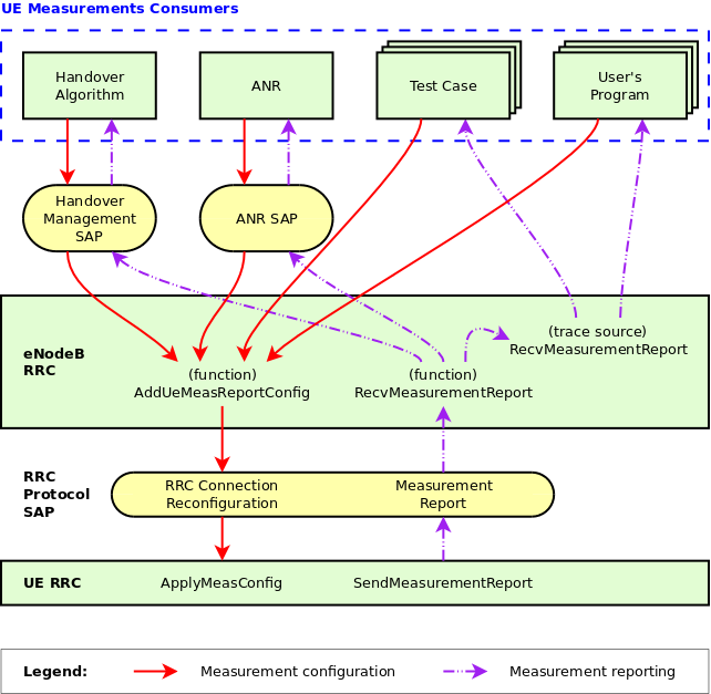
Relationship between UE measurements and its consumers
The whole UE measurements function at the RRC level is divided into 4 major parts:
- Measurement configuration (handled by
LteUeRrc::ApplyMeasConfig)- Performing measurements (handled by
LteUeRrc::DoReportUeMeasurements)- Measurement report triggering (handled by
LteUeRrc::MeasurementReportTriggering)- Measurement reporting (handled by
LteUeRrc::SendMeasurementReport)
The following sections will describe each of the parts above.
Measurement configuration
An eNodeB RRC entity configures UE measurements by sending the configuration
parameters to the UE RRC entity. This set of parameters are defined within the
MeasConfig Information Element (IE) of the RRC Connection Reconfiguration
message (RRC connection reconfiguration).
The eNodeB RRC entity implements the configuration parameters and procedures described in Section 5.5.2 of [TS36331], with the following simplifying assumption:
- configuration (i.e. addition, modification, and removal) can only be done before the simulation begins;
- all UEs attached to the eNodeB will be configured the same way, i.e. there is no support for configuring specific measurement for specific UE; and
- it is assumed that there is a one-to-one mapping between the PCI and the E-UTRAN Global Cell Identifier (EGCI). This is consistent with the PCI modeling assumptions described in UE PHY Measurements Model.
The eNodeB RRC instance here acts as an intermediary between the consumers and the attached UEs. At the beginning of simulation, each consumer provides the eNodeB RRC instance with the UE measurements configuration that it requires. After that, the eNodeB RRC distributes the configuration to attached UEs.
Users may customize the measurement configuration using several methods. Please refer to Section Configure UE measurements of the User Documentation for the description of these methods.
Performing measurements
UE RRC receives both RSRP and RSRQ measurements on periodical basis from UE PHY, as described in UE PHY Measurements Model. Layer 3 filtering will be applied to these received measurements. The implementation of the filtering follows Section 5.5.3.2 of [TS36331]:

where:
is the latest received measurement result from the physical layer;
is the updated filtered measurement result;
is the old filtered measurement result, where
(i.e. the first measurement is not filtered); and
, where
QuantityConfig;
 is the default value, but can be configured by setting the
RsrpFilterCoefficient and RsrqFilterCoefficient attributes in
is the default value, but can be configured by setting the
RsrpFilterCoefficient and RsrqFilterCoefficient attributes in
LteEnbRrc.
Therefore  will disable Layer 3 filtering. On the other hand, past
measurements can be granted more influence on the filtering results by using
larger value of .
will disable Layer 3 filtering. On the other hand, past
measurements can be granted more influence on the filtering results by using
larger value of .
Measurement reporting triggering
In this part, UE RRC will go through the list of active measurement configuration and check whether the triggering condition is fulfilled in accordance with Section 5.5.4 of [TS36331]. When at least one triggering condition from all the active measurement configuration is fulfilled, the measurement reporting procedure (described in the next subsection) will be initiated.
3GPP defines two kinds of triggerType: periodical and event-based. At the moment, only event-based criterion is supported. There are various events that can be selected, which are briefly described in the table below:
| Name | Description |
|---|---|
| Event A1 | Serving cell becomes better than threshold |
| Event A2 | Serving cell becomes worse than threshold |
| Event A3 | Neighbour becomes offset dB better than serving cell |
| Event A4 | Neighbour becomes better than threshold |
| Event A5 | Serving becomes worse than threshold1 AND neighbour becomes better than threshold2 |
Two main conditions to be checked in an event-based trigger are the entering condition and the leaving condition. More details on these two can be found in Section 5.5.4 of [TS36331].
An event-based trigger can be further configured by introducing hysteresis and
time-to-trigger. Hysteresis ( ) defines the distance between the
entering and leaving conditions in dB. Similarly, time-to-trigger introduces
delay to both entering and leaving conditions, but as a unit of time.
) defines the distance between the
entering and leaving conditions in dB. Similarly, time-to-trigger introduces
delay to both entering and leaving conditions, but as a unit of time.
The periodical type of reporting trigger is not supported, but its behavior
can be easily obtained by using an event-based trigger. This can be done by
configuring the measurement in such a way that the entering condition is always
fulfilled, for example, by setting the threshold of Event A1 to zero (the
minimum level). As a result, the measurement reports will always be triggered
at every certain interval, as determined by the reportInterval field within
LteRrcSap::ReportConfigEutra, therefore producing the same behaviour as
periodical reporting.
As a limitation with respect to 3GPP specifications, the current model does not
support any cell-specific configuration. These configuration parameters are
defined in measurement object. As a consequence, incorporating a list of black
cells into the triggering process is not supported. Moreover, cell-specific
offset (i.e.,  and
and  in Event A3, A4, and A5) are not
supported as well. The value equal to zero is always assumed in place of them.
in Event A3, A4, and A5) are not
supported as well. The value equal to zero is always assumed in place of them.
Measurement reporting
This part handles the submission of measurement report from the UE RRC entity to the serving eNodeB entity via RRC protocol. Several simplifying assumptions have been adopted:
- reportAmount is not applicable (i.e. always assumed to be infinite);
- in measurement reports, the reportQuantity is always assumed to be BOTH, i.e., both RSRP and RSRQ are always reported, regardless of the triggerQuantity.
Handover
The RRC model supports UE mobility in CONNECTED mode by invoking the X2-based handover procedure. The model is intra-EUTRAN and intra-frequency, as based on Section 10.1.2.1 of [TS36300].
This section focuses on the process of triggering a handover. The handover execution procedure itself is covered in Section X2.
There are two ways to trigger the handover procedure:
- explicitly (or manually) triggered by the simulation program by scheduling an execution of the method
LteEnbRrc::SendHandoverRequest; or- automatically triggered by the eNodeB RRC entity based on UE measurements and according to the selected handover algorithm.
Section X2-based handover of the User Documentation provides some examples on using both explicit and automatic handover triggers in simulation. The next subsection will take a closer look on the automatic method, by describing the design aspects of the handover algorithm interface and the available handover algorithms.
Handover algorithm
Handover in 3GPP LTE has the following properties:
- UE-assisted
- The UE provides input to the network in the form of measurement reports. This is handled by the UE RRC Measurements Model.
- Network-controlled
- The network (i.e. the source eNodeB and the target eNodeB) decides when to trigger the handover and oversees its execution.
The handover algorithm operates at the source eNodeB and is responsible in making handover decisions in an “automatic” manner. It interacts with an eNodeB RRC instance via the Handover Management SAP interface. These relationships are illustrated in Figure Relationship between UE measurements and its consumers from the previous section.
The handover algorithm interface consists of the following methods:
AddUeMeasReportConfigForHandover- (Handover Algorithm -> eNodeB RRC) Used by the handover algorithm to request measurement reports from the eNodeB RRC entity, by passing the desired reporting configuration. The configuration will be applied to all future attached UEs.
ReportUeMeas- (eNodeB RRC -> Handover Algorithm) Based on the UE measurements configured earlier in
AddUeMeasReportConfigForHandover, UE may submit measurement reports to the eNodeB. The eNodeB RRC entity uses theReportUeMeasinterface to forward these measurement reports to the handover algorithm.
TriggerHandover- (Handover Algorithm -> eNodeB RRC) After examining the measurement reports (but not necessarily), the handover algorithm may declare a handover. This method is used to notify the eNodeB RRC entity about this decision, which will then proceed to commence the handover procedure.
One note for the AddUeMeasReportConfigForHandover. The method will return
the measId (measurement identity) of the newly created measurement
configuration. Typically a handover algorithm would store this unique number. It
may be useful in the ReportUeMeas method, for example when more than one
configuration has been requested and the handover algorithm needs to
differentiate incoming reports based on the configuration that triggered them.
A handover algorithm is implemented by writing a subclass of the
LteHandoverAlgorithm abstract superclass and implementing each of the above
mentioned SAP interface methods. Users may develop their own handover algorithm
this way, and then use it in any simulation by following the steps outlined in
Section X2-based handover of the User Documentation.
Alternatively, users may choose to use one of the 3 built-in handover algorithms provided by the LTE module: no-op, A2-A4-RSRQ, and strongest cell handover algorithm. They are ready to be used in simulations or can be taken as an example of implementing a handover algorithm. Each of these built-in algorithms is covered in each of the following subsections.
No-op handover algorithm
The no-op handover algorithm (NoOpHandoverAlgorithm class) is the simplest
possible implementation of handover algorithm. It basically does nothing, i.e.,
does not call any of the Handover Management SAP interface methods. Users may
choose this handover algorithm if they wish to disable automatic handover
trigger in their simulation.
A2-A4-RSRQ handover algorithm
The A2-A4-RSRQ handover algorithm provides the functionality of the default
handover algorithm originally included in LENA M6 (ns-3.18), ported to the
Handover Management SAP interface as the A2A4RsrqHandoverAlgorithm class.
As the name implies, the algorithm utilizes the Reference Signal Received Quality (RSRQ) measurements acquired from Event A2 and Event A4. Thus, the algorithm will add 2 measurement configuration to the corresponding eNodeB RRC instance. Their intended use are described as follows:
- Event A2 (serving cell’s RSRQ becomes worse than threshold) is leveraged to indicate that the UE is experiencing poor signal quality and may benefit from a handover.
- Event A4 (neighbour cell’s RSRQ becomes better than threshold) is used to detect neighbouring cells and acquire their corresponding RSRQ from every attached UE, which are then stored internally by the algorithm. By default, the algorithm configures Event A4 with a very low threshold, so that the trigger criteria are always true.
Figure A2-A4-RSRQ handover algorithm below summarizes this procedure.
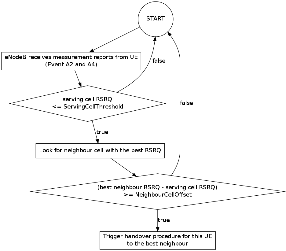
A2-A4-RSRQ handover algorithm
Two attributes can be set to tune the algorithm behaviour:
ServingCellThreshold- The threshold for Event A2, i.e. a UE must have an RSRQ lower than this threshold to be considered for a handover.
NeighbourCellOffset- The offset that aims to ensure that the UE would receive better signal quality after the handover. A neighbouring cell is considered as a target cell for the handover only if its RSRQ is higher than the serving cell’s RSRQ by the amount of this offset.
The value of both attributes are expressed as RSRQ range (Section 9.1.7 of [TS36133]), which is an integer between 0 and 34, with 0 as the lowest RSRQ.
Strongest cell handover algorithm
The strongest cell handover algorithm, or also sometimes known as the traditional power budget (PBGT) algorithm, is developed using [Dimou2009] as reference. The idea is to provide each UE with the best possible Reference Signal Received Power (RSRP). This is done by performing a handover as soon as a better cell (i.e. with stronger RSRP) is detected.
Event A3 (neighbour cell’s RSRP becomes better than serving cell’s RSRP) is
chosen to realize this concept. The A3RsrpHandoverAlgorithm class is the
result of the implementation. Handover is triggered for the UE to the best cell
in the measurement report.
A simulation which uses this algorithm is usually more vulnerable to ping-pong handover (consecutive handover to the previous source eNodeB within short period of time), especially when the Fading Model is enabled. This problem is typically tackled by introducing a certain delay to the handover. The algorithm does this by including hysteresis and time-to-trigger parameters (Section 6.3.5 of [TS36331]) to the UE measurements configuration.
Hysteresis (a.k.a. handover margin) delays the handover in regard of RSRP. The value is expressed in dB, ranges between 0 to 15 dB, and have a 0.5 dB accuracy, e.g., an input value of 2.7 dB is rounded to 2.5 dB.
On the other hand, time-to-trigger delays the handover in regard of time. 3GPP defines 16 valid values for time-to-trigger (all in milliseconds): 0, 40, 64, 80, 100, 128, 160, 256, 320, 480, 512, 640, 1024, 1280, 2560, and 5120.
The difference between hysteresis and time-to-trigger is illustrated in Figure Effect of hysteresis and time-to-trigger in strongest cell handover algorithm below, which is taken from the lena-x2-handover-measures example. It depicts the perceived RSRP of serving cell and a neighbouring cell by a UE which moves pass the border of the cells.
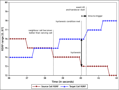
Effect of hysteresis and time-to-trigger in strongest cell handover algorithm
By default, the algorithm uses a hysteresis of 3.0 dB and time-to-trigger of
256 ms. These values can be tuned through the Hysteresis and
TimeToTrigger attributes of the A3RsrpHandoverAlgorithm class.
Neighbour Relation
LTE module supports a simplified Automatic Neighbour Relation (ANR) function.
This is handled by the LteAnr class, which interacts with an eNodeB RRC
instance through the ANR SAP interface.
Neighbour Relation Table
The ANR holds a Neighbour Relation Table (NRT), similar to the description in Section 22.3.2a of [TS36300]. Each entry in the table is called a Neighbour Relation (NR) and represents a detected neighbouring cell, which contains the following boolean fields:
- No Remove
- Indicates that the NR shall not be removed from the NRT. This is true by default for user-provided NR and false otherwise.
- No X2
- Indicates that the NR shall not use an X2 interface in order to initiate procedures towards the eNodeB parenting the target cell. This is false by default for user-provided NR, and true otherwise.
- No HO
- Indicates that the NR shall not be used by the eNodeB for handover reasons. This is true in most cases, except when the NR is both user-provided and network-detected.
Each NR entry may have at least one of the following properties:
- User-provided
- This type of NR is created as instructed by the simulation user. For example, a NR is created automatically upon a user-initiated establishment of X2 connection between 2 eNodeBs, e.g. as described in Section X2-based handover. Another way to create a user-provided NR is to call the
AddNeighbourRelationfunction explicitly.
- Network-detected
- This type of NR is automatically created during the simulation as a result of the discovery of a nearby cell.
In order to automatically create network-detected NR, ANR utilizes UE
measurements. In other words, ANR is a consumer of UE measurements, as depicted
in Figure Relationship between UE measurements and its consumers. RSRQ and Event A4 (neighbour becomes
better than threshold) are used for the reporting configuration. The default
Event A4 threshold is set to the lowest possible, i.e., maximum detection
capability, but can be changed by setting the Threshold attribute of
LteAnr class. Note that the A2-A4-RSRQ handover algorithm also utilizes a
similar reporting configuration. Despite the similarity, when both ANR and this
handover algorithm are active in the eNodeB, they use separate reporting
configuration.
Also note that automatic setup of X2 interface is not supported. This is the reason why the No X2 and No HO fields are true in a network-detected but not user-detected NR.
Role of ANR in Simulation
The ANR SAP interface provides the means of communication between ANR and eNodeB RRC. Some interface functions are used by eNodeB RRC to interact with the NRT, as shown below:
AddNeighbourRelation- (eNodeB RRC -> ANR) Add a new user-provided NR entry into the NRT.
GetNoRemove- (eNodeB RRC -> ANR) Get the value of No Remove field of an NR entry of the given cell ID.
GetNoHo- (eNodeB RRC -> ANR) Get the value of No HO field of an NR entry of the given cell ID.
GetNoX2- (eNodeB RRC -> ANR) Get the value of No X2 field of an NR entry of the given cell ID.
Other interface functions exist to support the role of ANR as a UE measurements consumer, as listed below:
AddUeMeasReportConfigForAnr- (ANR -> eNodeB RRC) Used by the ANR to request measurement reports from the eNodeB RRC entity, by passing the desired reporting configuration. The configuration will be applied to all future attached UEs.
ReportUeMeas- (eNodeB RRC -> ANR) Based on the UE measurements configured earlier in
AddUeMeasReportConfigForAnr, UE may submit measurement reports to the eNodeB. The eNodeB RRC entity uses theReportUeMeasinterface to forward these measurement reports to the ANR.
Please refer to the corresponding API documentation for LteAnrSap class for
more details on the usage and the required parameters.
The ANR is utilized by the eNodeB RRC instance as a data structure to keep track of the situation of nearby neighbouring cells. The ANR also helps the eNodeB RRC instance to determine whether it is possible to execute a handover procedure to a neighbouring cell. This is realized by the fact that eNodeB RRC will only allow a handover procedure to happen if the NR entry of the target cell has both No HO and No X2 fields set to false.
ANR is enabled by default in every eNodeB instance in the simulation. It can be
disabled by setting the AnrEnabled attribute in LteHelper class to
false.
RRC sequence diagrams
In this section we provide some sequence diagrams that explain the most important RRC procedures being modeled.
RRC connection establishment
Figure Sequence diagram of the RRC Connection Establishment procedure shows how the RRC Connection Establishment procedure is modeled, highlighting the role of the RRC layer at both the UE and the eNB, as well as the interaction with the other layers.
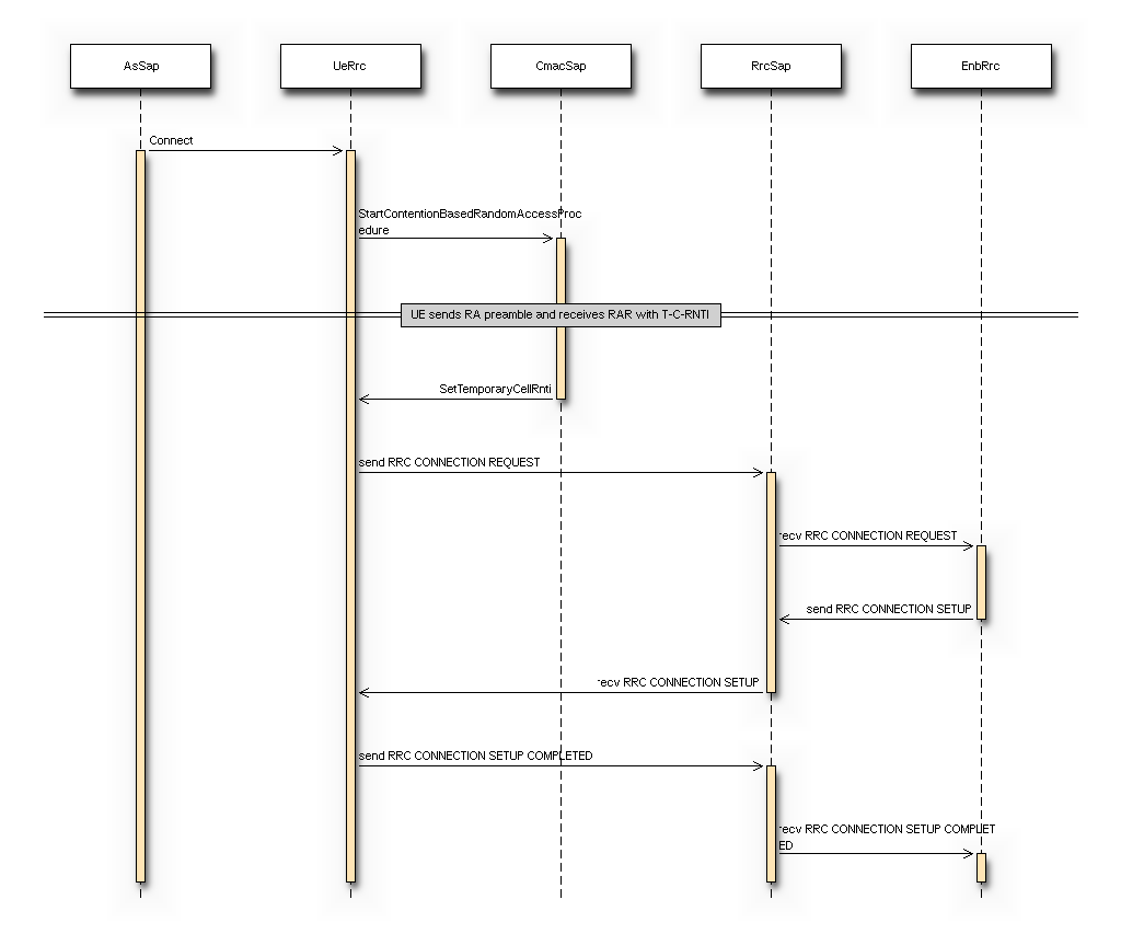
Sequence diagram of the RRC Connection Establishment procedure
There are several timeouts related to this procedure, which are listed in the following Table Timers in RRC connection establishment procedure. If any of these timers expired, the RRC connection establishment procedure is terminated in failure. At the UE side, if T300 timer has expired a consecutive connEstFailCount times on the same cell it performs the cell selection again [TS36331]. Else, the upper layer (UE NAS) will immediately attempt to retry the procedure.
| Name | Location | Timer starts | Timer stops | Default duration | When timer expired |
|---|---|---|---|---|---|
| Connection request timeout | eNodeB RRC | New UE context added | Receive RRC CONNECTION REQUEST | 15 ms (Max) | Remove UE context |
| Connection timeout (T300 timer) | UE RRC | Send RRC CONNECTION REQUEST | Receive RRC CONNECTION SETUP or REJECT | 100 ms | Reset UE MAC |
| Connection setup timeout | eNodeB RRC | Send RRC CONNECTION SETUP | Receive RRC CONNECTION SETUP COMPLETE | 100 ms | Remove UE context |
| Connection rejected timeout | eNodeB RRC | Send RRC CONNECTION REJECT | Never | 30 ms | Remove UE context |
Note: The value of connection request timeout timer at the eNB RRC should
not be higher than the T300 timer at UE RRC. It is to make sure that the UE
context is already removed at the eNB, once the UE will perform cell selection
upon reaching the connEstFailCount count. Moreover, at the time of writing
this document the Cell Selection Evaluation does not include
the  parameter, thus, it is not applied while selecting
the same cell again.
parameter, thus, it is not applied while selecting
the same cell again.
| Name | Location | Msg | Monitored by | Default value | Limit not reached | Limit reached |
|---|---|---|---|---|---|---|
| ConnEstFailCount | eNB MAC | RachConfigCommon in SIB2, HO REQ and HO Ack | UE RRC | 1 | Increment the local counter. Invalided the prev SIB2 msg, and try random access with the same cell. | Reset the local counter and perform cell selection. |
RRC connection reconfiguration
Figure Sequence diagram of the RRC Connection Reconfiguration procedure shows how the RRC Connection Reconfiguration procedure is modeled for the case where MobilityControlInfo is not provided, i.e., handover is not performed.
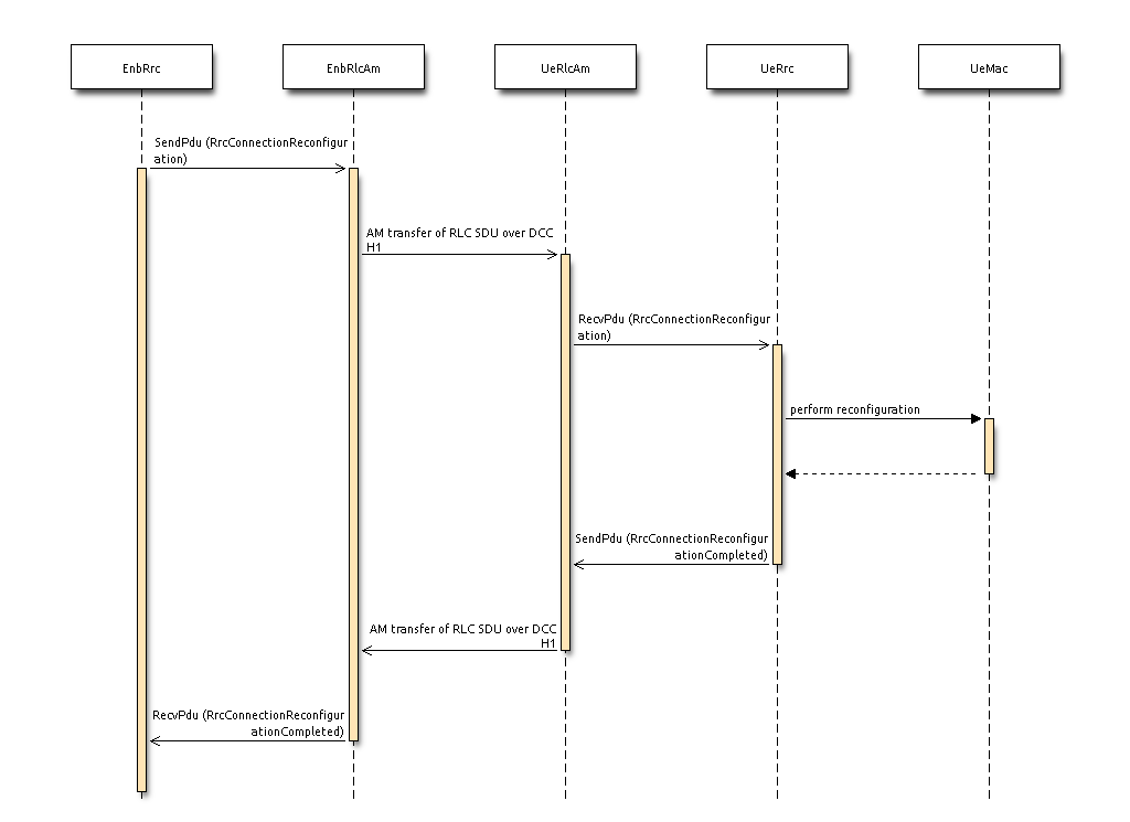
Sequence diagram of the RRC Connection Reconfiguration procedure
Figure Sequence diagram of the RRC Connection Reconfiguration procedure for the handover case shows how the RRC Connection Reconfiguration procedure is modeled for the case where MobilityControlInfo is provided, i.e., handover is to be performed. As specified in [TS36331], After receiving the handover message, the UE attempts to access the target cell at the first available RACH occasion according to Random Access resource selection defined in [TS36321]_, i.e. the handover is asynchronous. Consequently, when allocating a dedicated preamble for the random access in the target cell, E-UTRA shall ensure it is available from the first RACH occasion the UE may use. Upon successful completion of the handover, the UE sends a message used to confirm the handover. Note that the random access procedure in this case is non-contention based, hence in a real LTE system it differs slightly from the one used in RRC connection established. Also note that the RA Preamble ID is signaled via the Handover Command included in the X2 Handover Request ACK message sent from the target eNB to the source eNB; in particular, the preamble is included in the RACH-ConfigDedicated IE which is part of MobilityControlInfo.
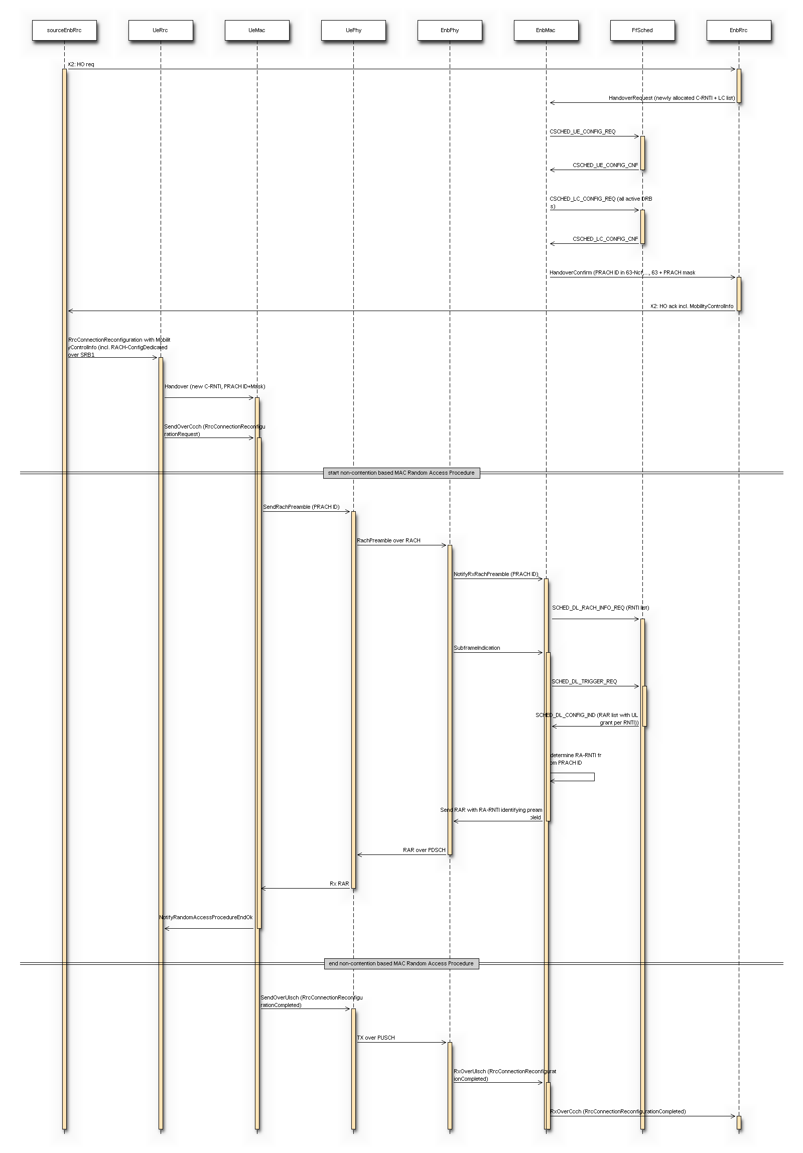
Sequence diagram of the RRC Connection Reconfiguration procedure for the handover case
RRC protocol models
As previously anticipated, we provide two different models for the transmission and reception of RRC messages: Ideal and Real. Each of them is described in one of the following subsections.
Ideal RRC protocol model
According to this model, implemented in the classes and LteUeRrcProtocolIdeal and LteEnbRrcProtocolIdeal, all RRC messages and information elements are transmitted between the eNB and the UE in an ideal fashion, without consuming radio resources and without errors. From an implementation point of view, this is achieved by passing the RRC data structure directly between the UE and eNB RRC entities, without involving the lower layers (PDCP, RLC, MAC, scheduler).
Real RRC protocol model
This model is implemented in the classes LteUeRrcProtocolReal and LteEnbRrcProtocolReal and aims at modeling the transmission of RRC PDUs as commonly performed in real LTE systems. In particular:
- for every RRC message being sent, a real RRC PDUs is created following the ASN.1 encoding of RRC PDUs and information elements (IEs) specified in [TS36331]. Some simplification are made with respect to the IEs included in the PDU, i.e., only those IEs that are useful for simulation purposes are included. For a detailed list, please see the IEs defined in lte-rrc-sap.h and compare with [TS36331].
- the encoded RRC PDUs are sent on Signaling Radio Bearers and are subject to the same transmission modeling used for data communications, thus including scheduling, radio resource consumption, channel errors, delays, retransmissions, etc.
We now describe the Signaling Radio Bearer model that is used for the Real RRC protocol model.
SRB0 messages (over CCCH):
- RrcConnectionRequest: in real LTE systems, this is an RLC TM SDU sent over resources specified in the UL Grant in the RAR (not in UL DCIs); the reason is that C-RNTI is not known yet at this stage. In the simulator, this is modeled as a real RLC TM RLC PDU whose UL resources are allocated by the scheduler upon call to SCHED_DL_RACH_INFO_REQ.
- RrcConnectionSetup: in the simulator this is implemented as in real LTE systems, i.e., with an RLC TM SDU sent over resources indicated by a regular UL DCI, allocated with SCHED_DL_RLC_BUFFER_REQ triggered by the RLC TM instance that is mapped to LCID 0 (the CCCH).
SRB1 messages (over DCCH):
- All the SRB1 messages modeled in the simulator (e.g., RrcConnectionCompleted) are implemented as in real LTE systems, i.e., with a real RLC SDU sent over RLC AM using DL resources allocated via Buffer Status Reports. See the RLC model documentation for details.
SRB2 messages (over DCCH):
- According to [TS36331], “SRB1 is for RRC messages (which may include a piggybacked NAS message) as well as for NAS messages prior to the establishment of SRB2, all using DCCH logical channel”, whereas “SRB2 is for NAS messages, using DCCH logical channel” and “SRB2 has a lower-priority than SRB1 and is always configured by E-UTRAN after security activation”. Modeling security-related aspects is not a requirement of the LTE simulation model, hence we always use SRB1 and never activate SRB2.
The messages defined in RRC SAP, common to all Ue/Enb SAP Users/Providers, are transported in a transparent container to/from a Ue/Enb. The encoding format for the different Information Elements are specified in [TS36331], using ASN.1 rules in the unaligned variant. The implementation in Ns3/Lte has been divided in the following classes:
- Asn1Header : Contains the encoding / decoding of basic ASN types
- RrcAsn1Header : Inherits Asn1Header and contains the encoding / decoding of common IE’s defined in [TS36331]
- Rrc specific messages/IEs classes : A class for each of the messages defined in RRC SAP header
This class implements the methods to Serialize / Deserialize the ASN.1 types being used in [TS36331], according to the packed encoding rules in ITU-T X.691. The types considered are:
- Boolean : a boolean value uses a single bit (1=true, 0=false).
- Integer : a constrained integer (with min and max values defined) uses the minimum amount of bits to encode its range (max-min+1).
- Bitstring : a bistring will be copied bit by bit to the serialization buffer.
- Octetstring : not being currently used.
- Sequence : the sequence generates a preamble indicating the presence of optional and default fields. It also adds a bit indicating the presence of extension marker.
- Sequence…Of : the sequence…of type encodes the number of elements of the sequence as an integer (the subsequent elements will need to be encoded afterwards).
- Choice : indicates which element among the ones in the choice set is being encoded.
- Enumeration : is serialized as an integer indicating which value is used, among the ones in the enumeration, with the number of elements in the enumeration as upper bound.
- Null : the null value is not encoded, although its serialization function is defined to provide a clearer map between specification and implementation.
The class inherits from ns-3 Header, but Deserialize() function is declared pure virtual, thus inherited classes having to implement it. The reason is that deserialization will retrieve the elements in RRC messages, each of them containing different information elements.
Additionally, it has to be noted that the resulting byte length of a specific type/message can vary, according to the presence of optional fields, and due to the optimized encoding. Hence, the serialized bits will be processed using PreSerialize() function, saving the result in m_serializationResult Buffer. As the methods to read/write in a ns3 buffer are defined in a byte basis, the serialization bits are stored into m_serializationPendingBits attribute, until the 8 bits are set and can be written to buffer iterator. Finally, when invoking Serialize(), the contents of the m_serializationResult attribute will be copied to Buffer::Iterator parameter
As some Information Elements are being used for several RRC messages, this class implements the following common IE’s:
- SrbToAddModList
- DrbToAddModList
- LogicalChannelConfig
- RadioResourceConfigDedicated
- PhysicalConfigDedicated
- SystemInformationBlockType1
- SystemInformationBlockType2
- RadioResourceConfigCommonSIB
The following RRC SAP have been implemented:
- RrcConnectionRequest
- RrcConnectionSetup
- RrcConnectionSetupCompleted
- RrcConnectionReconfiguration
- RrcConnectionReconfigurationCompleted
- HandoverPreparationInfo
- RrcConnectionReestablishmentRequest
- RrcConnectionReestablishment
- RrcConnectionReestablishmentComplete
- RrcConnectionReestablishmentReject
- RrcConnectionRelease
NAS
The focus of the LTE-EPC model is on the NAS Active state, which corresponds to EMM Registered, ECM connected, and RRC connected. Because of this, the following simplifications are made:
- EMM and ECM are not modeled explicitly; instead, the NAS entity at the UE will interact directly with the MME to perform actions that are equivalent (with gross simplifications) to taking the UE to the states EMM Connected and ECM Connected;
- the NAS also takes care of multiplexing uplink data packets coming from the upper layers into the appropriate EPS bearer by using the Traffic Flow Template classifier (TftClassifier).
- the NAS does not support PLMN and CSG selection
- the NAS does not support any location update/paging procedure in idle mode
Figure Sequence diagram of the attach procedure shows how the simplified NAS model implements the attach procedure. Note that both the default and eventual dedicated EPS bearers are activated as part of this procedure.
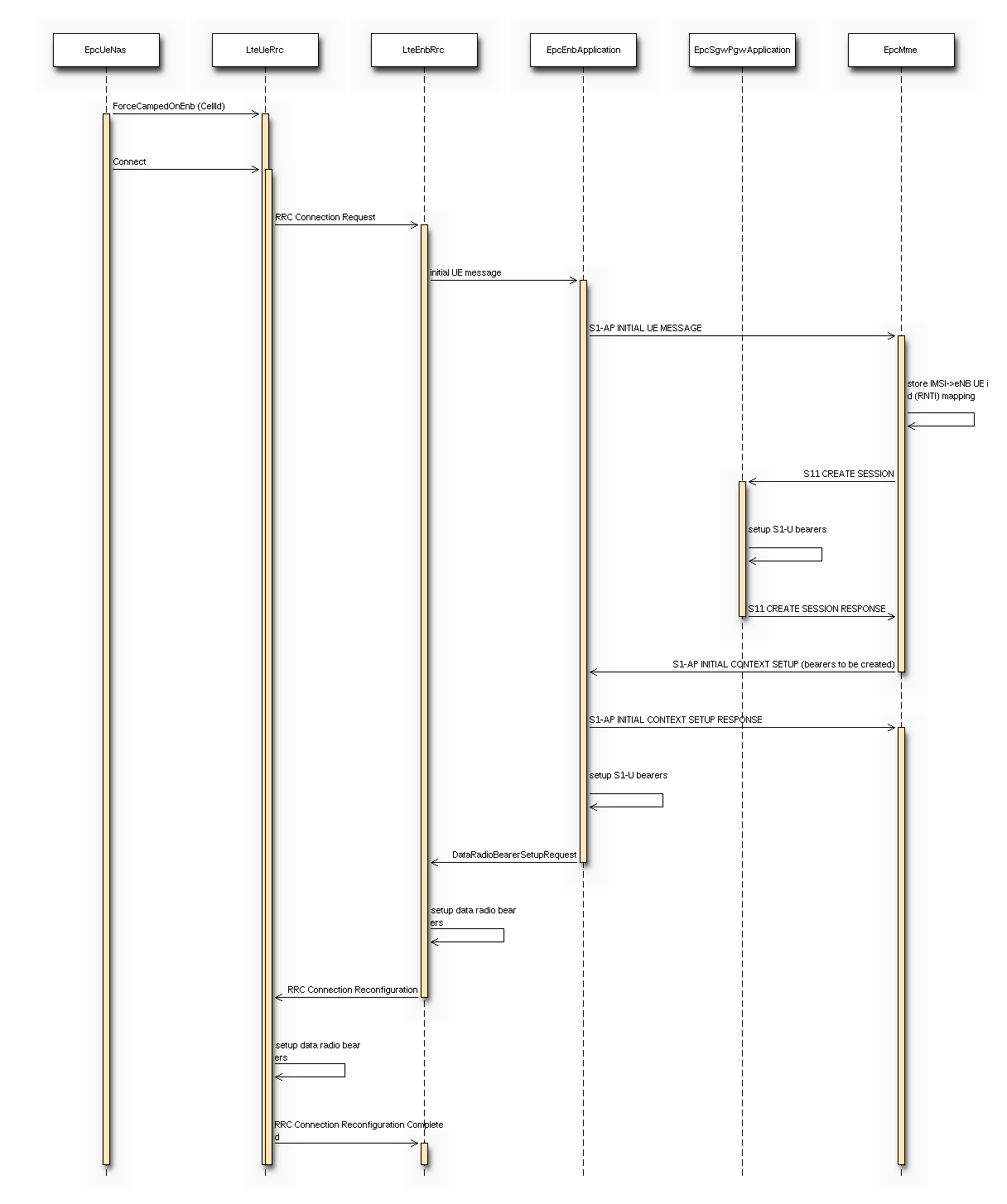
Sequence diagram of the attach procedure
S1, S5 and S11
S1-U and S5 (user plane)
The S1-U and S5 interfaces are modeled in a realistic way by encapsulating data packets over GTP/UDP/IP, as done in real LTE-EPC systems. The corresponding protocol stack is shown in Figure LTE-EPC data plane protocol stack. As shown in the figure, there are two different layers of IP networking. The first one is the end-to-end layer, which provides end-to-end connectivity to the users; this layer involves the UEs, the PGW and the remote host (including eventual internet routers and hosts in between), but does not involve the eNB and the SGW. In this version of LTE, the EPC supports both IPv4 and IPv6 type users. The 3GPP unique 64 bit IPv6 prefix allocation process for each UE and PGW is followed here. Each EPC is assigned a unique 16 bit IPv4 and a 48 bit IPv6 network address from the pool of 7.0.0.0/8 and 7777:f00d::/32 respectively. In the end-to-end IP connection between UE and PGW, all addresses are configured using these prefixes. The PGW’s address is used by all UEs as the gateway to reach the internet.
The second layer of IP networking is the EPC local area network. This involves all eNB nodes, SGW nodes and PGW nodes. This network is implemented as a set of point-to-point links which connect each eNB with its corresponding SGW node and a point-to-point link which connect each SGW node with its corresponding PGW node; thus, each SGW has a set of point-to-point devices, each providing connectivity to a different eNB. By default, a 10.x.y.z/30 subnet is assigned to each point-to-point link (a /30 subnet is the smallest subnet that allows for two distinct host addresses).
As specified by 3GPP, the end-to-end IP communications is tunneled over the local EPC IP network using GTP/UDP/IP. In the following, we explain how this tunneling is implemented in the EPC model. The explanation is done by discussing the end-to-end flow of data packets.
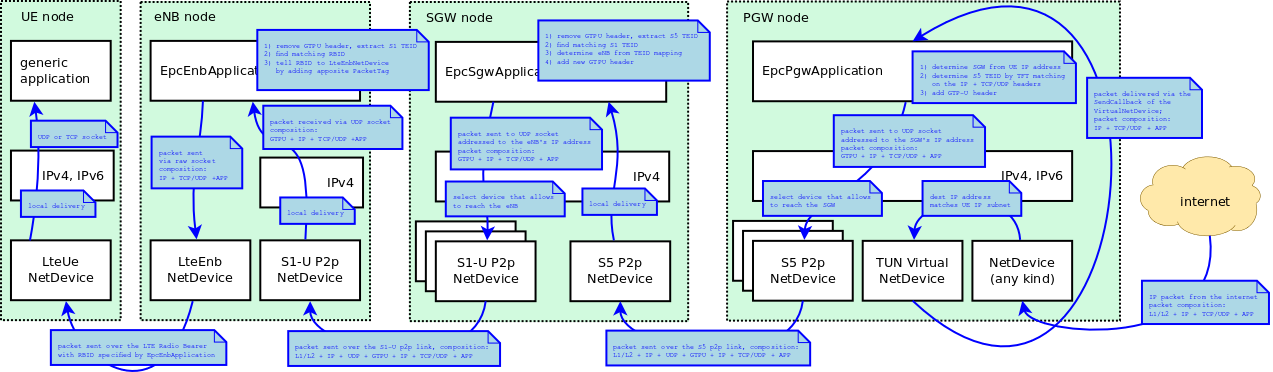
Data flow in the downlink between the internet and the UE
To begin with, we consider the case of the downlink, which is depicted in Figure Data flow in the downlink between the internet and the UE. Downlink IPv4/IPv6 packets are generated from a generic remote host, and addressed to one of the UE device. Internet routing will take care of forwarding the packet to the generic NetDevice of the PGW node which is connected to the internet (this is the Gi interface according to 3GPP terminology). The PGW has a VirtualNetDevice which is assigned the base IPv4 address of the EPC network; hence, static routing rules will cause the incoming packet from the internet to be routed through this VirtualNetDevice. In case of IPv6 address as destination, a manual route towards the VirtualNetDevice is inserted in the routing table, containing the 48 bit IPv6 prefix from which all the IPv6 addresses of the UEs and PGW are configured. Such device starts the GTP/UDP/IP tunneling procedure, by forwarding the packet to a dedicated application in the PGW node which is called EpcPgwApplication. This application does the following operations:
- it determines the SGW node to which it must route the traffic for this UE, by looking at the IP destination address (which is the address of the UE);
- it classifies the packet using Traffic Flow Templates (TFTs) to identify to which EPS Bearer it belongs. EPS bearers have a one-to-one mapping to S5 Bearers, so this operation returns the GTP-U Tunnel Endpoint Identifier (TEID) to which the packet belongs;
- it adds the corresponding GTP-U protocol header to the packet;
- finally, it sends the packet over a UDP socket to the S5 point-to-point NetDevice, addressed to the appropriate SGW.
As a consequence, the end-to-end IP packet with newly added IP, UDP and GTP headers is sent through one of the S5 links to the SGW, where it is received and delivered locally (as the destination address of the outermost IP header matches the SGW IP address). The local delivery process will forward the packet, via an UDP socket, to a dedicated application called EpcSgwApplication. This application then performs the following operations:
- it determines the eNB node to which the UE is attached, by looking at the S5 TEID;
- it maps the S5 TEID to get the S1 TEID. EPS bearers have a one-to-one mapping to S1-U Bearers, so this operation returns the S1 GTP-U Tunnel Endpoint Identifier (TEID) to which the packet belongs;
- it adds a new GTP-U protocol header to the packet;
- finally, it sends the packet over a UDP socket to the S1-U point-to-point NetDevice, addressed to the eNB to which the UE is attached.
Finally, the end-to-end IP packet with newly added IP, UDP and GTP headers is sent through one of the S1 links to the eNB, where it is received and delivered locally (as the destination address of the outermost IP header matches the eNB IP address). The local delivery process will forward the packet, via an UDP socket, to a dedicated application called EpcEnbApplication. This application then performs the following operations:
- it removes the GTP header and retrieves the S1 TEID which is contained in it;
- leveraging on the one-to-one mapping between S1-U bearers and Radio Bearers (which is a 3GPP requirement), it determines the Bearer ID (BID) to which the packet belongs;
- it records the BID in a dedicated tag called EpsBearerTag, which is added to the packet;
- it forwards the packet to the LteEnbNetDevice of the eNB node via a raw packet socket
Note that, at this point, the outmost header of the packet is the end-to-end IP header, since the IP/UDP/GTP headers of the S1 protocol stack have already been stripped. Upon reception of the packet from the EpcEnbApplication, the LteEnbNetDevice will retrieve the BID from the EpsBearerTag, and based on the BID will determine the Radio Bearer instance (and the corresponding PDCP and RLC protocol instances) which are then used to forward the packet to the UE over the LTE radio interface. Finally, the LteUeNetDevice of the UE will receive the packet, and delivery it locally to the IP protocol stack, which will in turn delivery it to the application of the UE, which is the end point of the downlink communication.
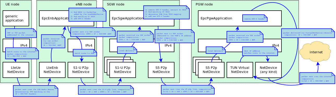
Data flow in the uplink between the UE and the internet
The case of the uplink is depicted in Figure Data flow in the uplink between the UE and the internet. Uplink IP packets are generated by a generic application inside the UE, and forwarded by the local TCP/IP stack to the LteUeNetDevice of the UE. The LteUeNetDevice then performs the following operations:
- it classifies the packet using TFTs and determines the Radio Bearer to which the packet belongs (and the corresponding RBID);
- it identifies the corresponding PDCP protocol instance, which is the entry point of the LTE Radio Protocol stack for this packet;
- it sends the packet to the eNB over the LTE Radio Protocol stack.
The eNB receives the packet via its LteEnbNetDevice. Since there is a single PDCP and RLC protocol instance for each Radio Bearer, the LteEnbNetDevice is able to determine the BID of the packet. This BID is then recorded onto an EpsBearerTag, which is added to the packet. The LteEnbNetDevice then forwards the packet to the EpcEnbApplication via a raw packet socket.
Upon receiving the packet, the EpcEnbApplication performs the following operations:
- it retrieves the BID from the EpsBearerTag in the packet;
- it determines the corresponding EPS Bearer instance and GTP-U TEID by leveraging on the one-to-one mapping between S1-U bearers and Radio Bearers;
- it adds a GTP-U header on the packet, including the TEID determined previously;
- it sends the packet to the SGW node via the UDP socket connected to the S1-U point-to-point net device.
At this point, the packet contains the S1-U IP, UDP and GTP headers in addition to the original end-to-end IP header. When the packet is received by the corresponding S1-U point-to-point NetDevice of the SGW node, it is delivered locally (as the destination address of the outmost IP header matches the address of the point-to-point net device). The local delivery process will forward the packet to the EpcSgwApplication via the corresponding UDP socket. The EpcSgwApplication then perfoms the following operations:
- it removes the GTP header and retrieves the S1-U TEID;
- it maps the S1-U TEID to get the S5 TEID to which the packet belongs;
- it determines the PGW to which it must send the packet from the TEID mapping;
- it add a new GTP-U protocol header to the packet;
- finally, it sends the packet over a UDP socket to the S5 point-to-point NetDevice, addressed to the corresponding PGW.
At this point, the packet contains the S5 IP, UDP and GTP headers in addition to the original end-to-end IP header. When the packet is received by the corresponding S5 point-to-point NetDevice of the PGW node, it is delivered locally (as the destination address of the outmost IP header matches the address of the point-to-point net device). The local delivery process will forward the packet to the EpcPgwApplication via the corresponding UDP socket. The EpcPgwApplication then removes the GTP header and forwards the packet to the VirtualNetDevice. At this point, the outmost header of the packet is the end-to-end IP header. Hence, if the destination address within this header is a remote host on the internet, the packet is sent to the internet via the corresponding NetDevice of the PGW. In the event that the packet is addressed to another UE, the IP stack of the PGW will redirect the packet again to the VirtualNetDevice, and the packet will go through the downlink delivery process in order to reach its destination UE.
Note that the EPS Bearer QoS is not enforced on the S1-U and S5 links, it is assumed that the overprovisioning of the link bandwidth is sufficient to meet the QoS requirements of all bearers.
S1AP
The S1-AP interface provides control plane interaction between the eNB and the MME. In the simulator, this interface is modeled in a realistic fashion transmitting the encoded S1AP messages and information elements specified in [TS36413] on the S1-MME link.
The S1-AP primitives that are modeled are:
- INITIAL UE MESSAGE
- INITIAL CONTEXT SETUP REQUEST
- INITIAL CONTEXT SETUP RESPONSE
- PATH SWITCH REQUEST
- PATH SWITCH REQUEST ACKNOWLEDGE
S5 and S11
The S5 interface provides control plane interaction between the SGW and the PGW. The S11 interface provides control plane interaction between the SGw and the MME. Both interfaces use the GPRS Tunneling Protocol (GTPv2-C) to tunnel signalling messages [TS29274] and use UDP as transport protocol. In the simulator, these interfaces and protocol are modeled in a realistic fashion transmitting the encoded GTP-C messages.
The GTPv2-C primitives that are modeled are:
- CREATE SESSION REQUEST
- CREATE SESSION RESPONSE
- MODIFY BEARER REQUEST
- MODIFY BEARER RESPONSE
- DELETE SESSION REQUEST
- DELETE SESSION RESPONSE
- DELETE BEARER COMMAND
- DELETE BEARER REQUEST
- DELETE BEARER RESPONSE
Of these primitives, the first two are used upon initial UE attachment for the establishment of the S1-U and S5 bearers. Section NAS shows the implementation of the attach procedure. The other primitives are used during the handover to switch the S1-U bearers from the source eNB to the target eNB as a consequence of the reception by the MME of a PATH SWITCH REQUEST S1-AP message.
X2
The X2 interface interconnects two eNBs [TS36420]. From a logical point of view, the X2 interface is a point-to-point interface between the two eNBs. In a real E-UTRAN, the logical point-to-point interface should be feasible even in the absence of a physical direct connection between the two eNBs. In the X2 model implemented in the simulator, the X2 interface is a point-to-point link between the two eNBs. A point-to-point device is created in both eNBs and the two point-to-point devices are attached to the point-to-point link.
For a representation of how the X2 interface fits in the overall architecture of the LENA simulation model, the reader is referred to the figure Overview of the LTE-EPC simulation model.
The X2 interface implemented in the simulator provides detailed implementation of the following elementary procedures of the Mobility Management functionality [TS36423]:
- Handover Request procedure
- Handover Request Acknowledgement procedure
- SN Status Transfer procedure
- UE Context Release procedure
These procedures are involved in the X2-based handover. You can find the detailed description of the handover in section 10.1.2.1 of [TS36300]. We note that the simulator model currently supports only the seamless handover as defined in Section 2.6.3.1 of [Sesia2009]; in particular, lossless handover as described in Section 2.6.3.2 of [Sesia2009] is not supported at the time of this writing.
Figure Sequence diagram of the X2-based handover below shows the interaction of the entities of the X2 model in the simulator. The shaded labels indicate the moments when the UE or eNodeB transition to another RRC state.
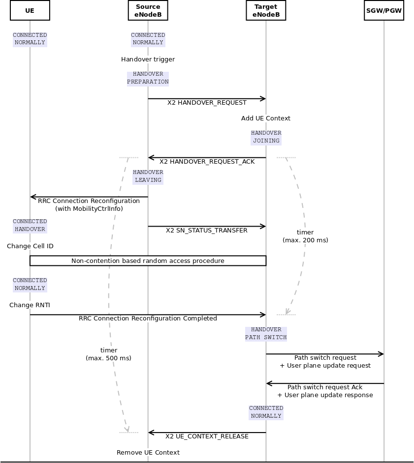
Sequence diagram of the X2-based handover
The figure also shows two timers within the handover procedure: the handover
leaving timer is maintained by the source eNodeB, while the handover joining
timer by the target eNodeB. The duration of the timers can be configured in
the HandoverLeavingTimeoutDuration and HandoverJoiningTimeoutDuration
attributes of the respective LteEnbRrc instances. When one of these timers
expire, the handover procedure is considered as failed.
However, there is no proper handling of handover failure in the current version of LTE module. Users should tune the simulation properly in order to avoid handover failure, otherwise unexpected behaviour may occur. Please refer to Section Tuning simulation with handover of the User Documentation for some tips regarding this matter.
The X2 model is an entity that uses services from:
- the X2 interfaces,
- They are implemented as Sockets on top of the point-to-point devices.
- They are used to send/receive X2 messages through the X2-C and X2-U interfaces (i.e. the point-to-point device attached to the point-to-point link) towards the peer eNB.
- the S1 application.
- Currently, it is the EpcEnbApplication.
- It is used to get some information needed for the Elementary Procedures of the X2 messages.
and it provides services to:
- the RRC entity (X2 SAP)
- to send/receive RRC messages. The X2 entity sends the RRC message as a transparent container in the X2 message. This RRC message is sent to the UE.
Figure Implementation Model of X2 entity and SAPs shows the implementation model of the X2 entity and its relationship with all the other entities and services in the protocol stack.
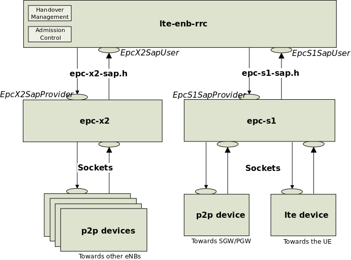
Implementation Model of X2 entity and SAPs
The RRC entity manages the initiation of the handover procedure. This is done in the Handover Management submodule of the eNB RRC entity. The target eNB may perform some Admission Control procedures. This is done in the Admission Control submodule. Initially, this submodule will accept any handover request.
X2 interfaces
The X2 model contains two interfaces:
- the X2-C interface. It is the control interface and it is used to send the X2-AP PDUs (i.e. the elementary procedures).
- the X2-U interface. It is used to send the bearer data when there is DL forwarding.
Figure X2 interface protocol stacks shows the protocol stacks of the X2-U interface and X2-C interface modeled in the simulator.
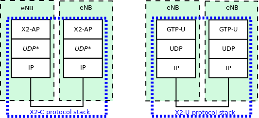
X2 interface protocol stacks
X2-C
The X2-C interface is the control part of the X2 interface and it is used to send the X2-AP PDUs (i.e. the elementary procedures).
In the original X2 interface control plane protocol stack, SCTP is used as the transport protocol but currently, the SCTP protocol is not modeled in the ns-3 simulator and its implementation is out-of-scope of the project. The UDP protocol is used as the datagram oriented protocol instead of the SCTP protocol.
X2-U
The X2-U interface is used to send the bearer data when there is DL forwarding during the execution of the X2-based handover procedure. Similarly to what done for the S1-U interface, data packets are encapsulated over GTP/UDP/IP when being sent over this interface. Note that the EPS Bearer QoS is not enforced on the X2-U links, it is assumed that the overprovisioning of the link bandwidth is sufficient to meet the QoS requirements of all bearers.
X2 Service Interface
The X2 service interface is used by the RRC entity to send and receive messages of the X2 procedures. It is divided into two parts:
- the
EpcX2SapProviderpart is provided by the X2 entity and used by the RRC entity and- the
EpcX2SapUserpart is provided by the RRC entity and used by the RRC enity.
The primitives that are supported in our X2-C model are described in the following subsections.
X2-C primitives for handover execution
The following primitives are used for the X2-based handover:
- HANDOVER REQUEST
- HANDOVER REQUEST ACK
- HANDOVER PREPARATION FAILURE
- SN STATUS STRANSFER
- UE CONTEXT RELEASE
all the above primitives are used by the currently implemented RRC model during the preparation and execution of the handover procedure. Their usage interacts with the RRC state machine; therefore, they are not meant to be used for code customization, at least unless it is desired to modify the RRC state machine.
X2-C SON primitives
The following primitives can be used to implement Self-Organized Network (SON) functionalities:
- LOAD INFORMATION
- RESOURCE STATUS UPDATE
note that the current RRC model does not actually use these primitives, they are included in the model just to make it possible to develop SON algorithms included in the RRC logic that make use of them.
As a first example, we show here how the load information primitive can be used. We assume that the LteEnbRrc has been modified to include the following new member variables:
std::vector<EpcX2Sap::UlInterferenceOverloadIndicationItem>
  m_currentUlInterferenceOverloadIndicationList;
std::vector <EpcX2Sap::UlHighInterferenceInformationItem>
  m_currentUlHighInterferenceInformationList;
EpcX2Sap::RelativeNarrowbandTxBand m_currentRelativeNarrowbandTxBand;
for a detailed description of the type of these variables, we suggest
to consult the file epc-x2-sap.h, the corresponding doxygen
documentation, and the references therein to the relevant sections of
3GPP TS 36.423. Now, assume that at run time these variables have been
set to meaningful values following the specifications just
mentioned. Then, you can add the following code in the LteEnbRrc class
implementation in order to send a load information primitive:
EpcX2Sap::CellInformationItem cii;
cii.sourceCellId = m_cellId;
cii.ulInterferenceOverloadIndicationList = m_currentUlInterferenceOverloadIndicationList;
cii.ulHighInterferenceInformationList = m_currentUlHighInterferenceInformationList;
cii.relativeNarrowbandTxBand = m_currentRelativeNarrowbandTxBand;

EpcX2Sap::LoadInformationParams params;
params.targetCellId = cellId;
params.cellInformationList.push_back (cii);
m_x2SapProvider->SendLoadInformation (params);
The above code allows the source eNB to send the message. The method
LteEnbRrc::DoRecvLoadInformation will be called when the target
eNB receives the message. The desired processing of the load
information should therefore be implemented within that method.
In the following second example we show how the resource status update primitive is used. We assume that the LteEnbRrc has been modified to include the following new member variable:
EpcX2Sap::CellMeasurementResultItem m_cmri;
similarly to before, we refer to epc-x2-sap.h and the references
therein for detailed information about this variable type.
Again, we assume that the variable has been already set to a
meaningful value. Then, you can add the following code in order to
send a resource status update:
EpcX2Sap::ResourceStatusUpdateParams params;
params.targetCellId = cellId;
params.cellMeasurementResultList.push_back (m_cmri);
m_x2SapProvider->SendResourceStatusUpdate (params);
The method eEnbRrc::DoRecvResourceStatusUpdate will be called when
the target eNB receives the resource status update message. The
desired processing of this message should therefore be implemented
within that method.
Finally, we note that the setting and processing of the appropriate values for the variable passed to the above described primitives is deemed to be specific of the SON algorithm being implemented, and hence is not covered by this documentation.
Unsupported primitives
Mobility Robustness Optimization primitives such as Radio Link Failure indication and Handover Report are not supported at this stage.
S11
The S11 interface provides control plane interaction between the SGW and the MME using the GTPv2-C protocol specified in [TS29274]. In the simulator, this interface is modeled in an ideal fashion, with direct interaction between the SGW and the MME objects, without actually implementing the encoding of the messages and without actually transmitting any PDU on any link.
The S11 primitives that are modeled are:
- CREATE SESSION REQUEST
- CREATE SESSION RESPONSE
- MODIFY BEARER REQUEST
- MODIFY BEARER RESPONSE
Of these primitives, the first two are used upon initial UE attachment for the establishment of the S1-U bearers; the other two are used during handover to switch the S1-U bearers from the source eNB to the target eNB as a consequence of the reception by the MME of a PATH SWITCH REQUEST S1-AP message.
Power Control
This section describes the ns-3 implementation of Downlink and Uplink Power Control.
Downlink Power Control
Since some of Frequency Reuse Algorithms require Downlink Power Control, this feature was also implemented in ns-3.
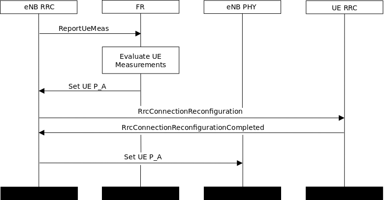
Sequence diagram of Downlink Power Control
Figure Sequence diagram of Downlink Power Control shows the sequence diagram of setting downlink P_A value for UE, highlighting the interactions between the RRC and the other entities. FR algorithm triggers RRC to change P_A values for UE. Then RRC starts RrcConnectionReconfiguration function to inform UE about new configuration. After successful RrcConnectionReconfiguration, RRC can set P_A value for UE by calling function SetPa from CphySap, value is saved in new map m_paMap which contain P_A values for each UE served by eNb.
When LteEnbPhy starts new subframe, DCI control messages are processed to get vector of used RBs. Now also GeneratePowerAllocationMap(uint16_t rnti, int rbId) function is also called. This function check P_A value for UE, generate power for each RB and store it in m_dlPowerAllocationMap. Then this map is used by CreateTxPowerSpectralDensityWithPowerAllocation function to create Ptr<SpectrumValue> txPsd.
PdschConfigDedicated (TS 36.331, 6.3.2 PDSCH-Config) was added in LteRrcSap::PhysicalConfigDedicated struct, which is used in RrcConnectionReconfiguration process.
Uplink Power Control
Uplink power control controls the transmit power of the different uplink physical channels. This functionality is described in 3GPP TS 36.213 section 5.
Uplink Power Control is enabled by default, and can be disabled by attribute system:
Config::SetDefault ("ns3::LteUePhy::EnableUplinkPowerControl", BooleanValue (false));
Two Uplink Power Control mechanisms are implemented:
- Open Loop Uplink Power Control: the UE transmission power depends on estimation of the downlink path-loss and channel configuration
- Closed Loop Uplink Power Control: as in Open Loop, in addition eNB can control the UE transmission power by means of explicit Transmit Power Control TPC commands transmitted in the downlink.
To switch between these two mechanism types, one should change parameter:
Config::SetDefault ("ns3::LteUePowerControl::ClosedLoop", BooleanValue (true));
By default, Closed Loop Power Control is enabled.
- Two modes of Closed Loop Uplink Power Control are available:
- Absolute mode: TxPower is computed with absolute TPC values
- Accumulative mode: TxPower is computed with accumulated TPC values
To switch between these two modes, one should change parameter:
Config::SetDefault ("ns3::LteUePowerControl::AccumulationEnabled", BooleanValue (true));
By default, Accumulation Mode is enabled and TPC commands in DL-DCI are set by all schedulers to 1, what is mapped to value of 0 in Accumulation Mode.
Uplink Power Control for PUSCH
The setting of the UE Transmit power for a Physical Uplink Shared Channel (PUSCH) transmission is defined as follows:
If the UE transmits PUSCH without a simultaneous PUCCH for the serving cell
, then the UE transmit power
for PUSCH transmission in subframe
If the UE transmits PUSCH simultaneous with PUCCH for the serving cell
Since Uplink Power Control for PUCCH is not implemented, this case is not implemented as well.
If the UE is not transmitting PUSCH for the serving cell
![P_{PUSCH,c}(i)=\min\begin{Bmatrix}
P_{CMAX,c}(i)\\
10\log_{10}(M_{PUSCH,c}(i))+ P_{O\_PUSCH,c}(j)
+ \alpha_{c} (j) * PL_{c} + \Delta_{TF,c}(i) + f_{c}(i)
\end{Bmatrix} [dBm]](_images/math/48fbe4d86c38694a906ce014d3586b83b043b70e.png)
![P_{PUSCH,c}(i)=\min\begin{Bmatrix}
10\log_{10}(\hat{P}_{CMAX,c}(i) - \hat{P}_{PUCCH}(i))\\
10\log_{10}(M_{PUSCH,c}(i))+ P_{O\_PUSCH,c}(j)
+ \alpha_{c} (j) * PL_{c} + \Delta_{TF,c}(i) + f_{c}(i)
\end{Bmatrix} [dBm]](_images/math/485d89cc67fe59bbf2b5c134cef849014b221af0.png)
![P_{PUSCH,c}(i)=\min\begin{Bmatrix}
{P}_{CMAX,c}(i)\\
P_{O\_PUSCH,c}(1) + \alpha_{c} (1) * PL_{c} + f_{c}(i)
\end{Bmatrix} [dBm]](_images/math/78ab89ef67195272913d0802f51cb08d07e60fdb.png)
- where:
 is the configured UE transmit power defined in 3GPP 36.101. Table 6.2.2-1
in subframe for serving cell and
is the configured UE transmit power defined in 3GPP 36.101. Table 6.2.2-1
in subframe for serving cell and  is the linear
value of . Default value for is 23 dBm
is the linear
value of . Default value for is 23 dBm is the bandwidth of the PUSCH resource assignment expressed in number
of resource blocks valid for subframe and serving cell .
is the bandwidth of the PUSCH resource assignment expressed in number
of resource blocks valid for subframe and serving cell . is a parameter composed of the sum of a component
  provided from higher layers for
  and a component
  provided by higher
layers for for serving cell . SIB2 message needs to be extended to carry these two
components, but currently they can be set via attribute system:
provided by higher
layers for for serving cell . SIB2 message needs to be extended to carry these two
components, but currently they can be set via attribute system:Config::SetDefault ("ns3::LteUePowerControl::PoNominalPusch", IntegerValue (-90)); Config::SetDefault ("ns3::LteUePowerControl::PoUePusch", IntegerValue (7));
 is a 3-bit parameter provided by higher layers for serving cell .
For
is a 3-bit parameter provided by higher layers for serving cell .
For  ,
,  For
For  ,
,  .
This parameter is configurable by attribute system:
.
This parameter is configurable by attribute system:Config::SetDefault ("ns3::LteUePowerControl::Alpha", DoubleValue (0.8));
 is the downlink pathloss estimate calculated in the UE for serving cell in dB
and
is the downlink pathloss estimate calculated in the UE for serving cell in dB
and  , where
  is provided by higher layers and RSRP. is provided in SIB2 message
 for
for  and
and  for
for  . Only second case is implemented.
 is component of Closed Loop Power Control. It is the current PUSCH power control
adjustment state for serving cell .
is component of Closed Loop Power Control. It is the current PUSCH power control
adjustment state for serving cell .If Accumulation Mode is enabled
is given by:
where:
 is a correction value, also referred to as a TPC command and is included
in PDCCH with DCI;
is a correction value, also referred to as a TPC command and is included
in PDCCH with DCI;  was signalled on PDCCH/EPDCCH with DCI for
serving cell on subframe
was signalled on PDCCH/EPDCCH with DCI for
serving cell on subframe  ;
;  for FDD.
If UE has reached
for serving cell , positive TPC commands for serving cell
are not be accumulated. If UE has reached minimum power, negative TPC commands are not be accumulated.
Minimum UE power is defined in TS36.101 section 6.2.3. Default value is -40 dBm.If Accumulation Mode is not enabled
is given by:
where:
is a correction value, also referred to as a TPC command and is included
in PDCCH with DCI; was signalled on PDCCH/EPDCCH with DCI for
serving cell on subframe ; for FDD.Mapping of TPC Command Field in DCI format 0/3/4 to absolute and accumulated
values is defined in TS36.231 section 5.1.1.1 Table 5.1.1.1-2
Uplink Power Control for PUCCH
Since all uplink control messages are an ideal messages and do not consume any radio resources, Uplink Power Control for PUCCH is not needed and it is not implemented.
Uplink Power Control for SRS
The setting of the UE Transmit power  for the SRS transmitted on subframe
for serving cell is defined by
for the SRS transmitted on subframe
for serving cell is defined by
![P_{PUSCH,c}(i)=\min\begin{Bmatrix}
{P}_{CMAX,c}(i)\\
P_{SRS\_OFFSET,c}(m) + 10\log_{10}(M_{SRS,c})+
P_{O\_PUSCH,c}(j) + \alpha_{c}(j) * PL_{c} + f_{c}(i)
\end{Bmatrix} [dBm]](_images/math/64cc6f41c617ec4064de08b9a784264a1d6794c4.png)
- where:
- is the configured UE transmit power defined in 3GPP 36.101. Table 6.2.2-1.
Default value for is 23 dBm
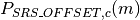 is semi-statically configured by higher layers for
  for
serving cell . For SRS transmission given trigger type 0 then and for SRS
transmission given trigger type 1 then
for
serving cell . For SRS transmission given trigger type 0 then and for SRS
transmission given trigger type 1 then  .
For P_Srs_Offset_Value is computed with equation:
.
For P_Srs_Offset_Value is computed with equation:![P_{SRS\_OFFSET,c}(m)value = -10.5 + P_{SRS\_OFFSET,c}(m) * 1.5 [dBm]](_images/math/0b57d02c0e1fcefe9fd49616806e4a7bcbc69db5.png)
This parameter is configurable by attribute system:
Config::SetDefault ("ns3::LteUePowerControl::PsrsOffset", IntegerValue (7));
 is the bandwidth of the SRS transmission in subframe for serving
cell expressed in number of resource blocks. In current implementation SRS is sent
over entire UL bandwidth.
is the bandwidth of the SRS transmission in subframe for serving
cell expressed in number of resource blocks. In current implementation SRS is sent
over entire UL bandwidth.- is the current PUSCH power control adjustment state for serving cell ,
as defined in Uplink Power Control for PUSCH
- and
 are parameters as defined in
Uplink Power Control for PUSCH, where
are parameters as defined in
Uplink Power Control for PUSCH, where  .
.
Fractional Frequency Reuse
Overview
This section describes the ns-3 support for Fractional Frequency Reuse algorithms. All implemented algorithms are described in [ASHamza2013]. Currently 7 FR algorithms are implemented:
ns3::LteFrNoOpAlgorithmns3::LteFrHardAlgorithmns3::LteFrStrictAlgorithmns3::LteFrSoftAlgorithmns3::LteFfrSoftAlgorithmns3::LteFfrEnhancedAlgorithmns3::LteFfrDistributedAlgorithm
New LteFfrAlgorithm class was created and it is a abstract class for Frequency Reuse algorithms implementation. Also, two new SAPs between FR-Scheduler and FR-RRC were added.
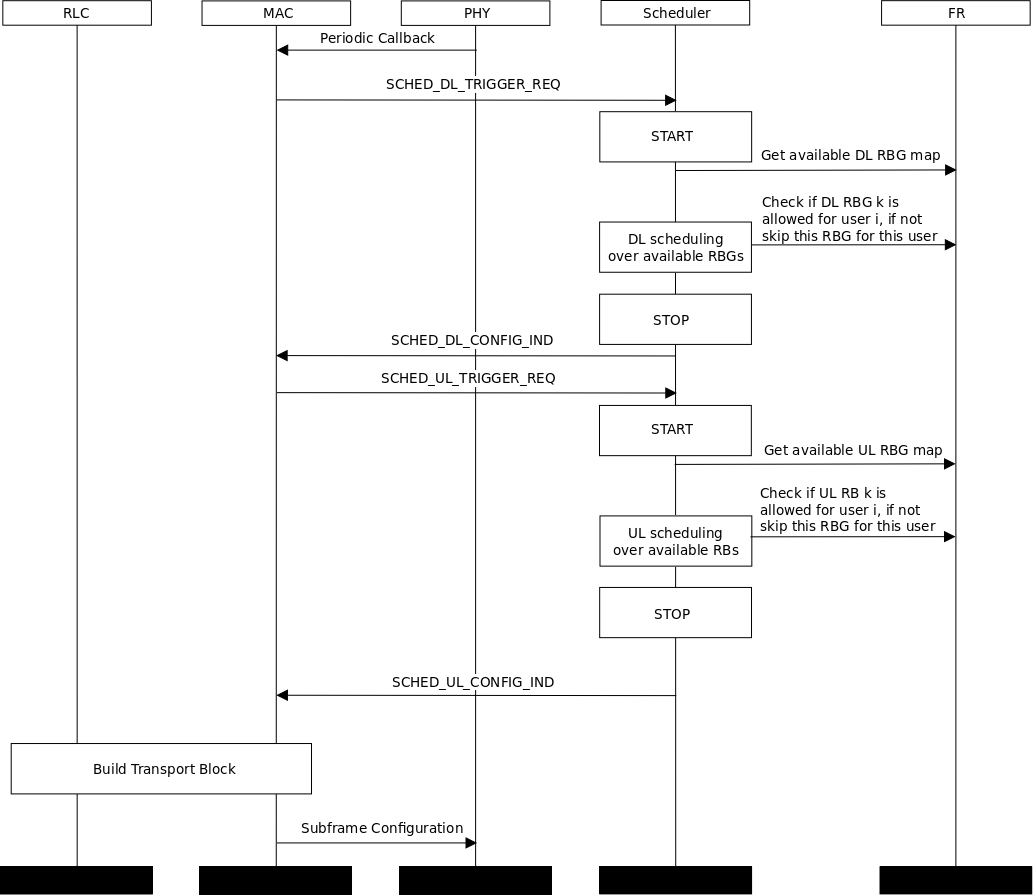
Sequence diagram of Scheduling with FR algorithm
Figure Sequence diagram of Scheduling with FR algorithm shows the sequence diagram of scheduling process with FR algorithm. In the beginning of scheduling process, scheduler asks FR entity for available RBGs. According to implementation FR returns all RBGs available in cell or filter them based on its policy. Then when trying to assign some RBG to UE, scheduler asks FR entity if this RBG is allowed for this UE. When FR returns true, scheduler can assign this RBG to this UE, if not scheduler is checking another RBG for this UE. Again, FR response depends on implementation and policy applied to UE.
Supported FR algorithms
No Frequency Reuse
The NoOp FR algorithm (LteFrNoOpAlgorithm class) is implementation of Full Frequency Reuse scheme, that means no frequency partitioning is performed between eNBs of the same network (frequency reuse factor, FRF equals 1). eNBs uses entire system bandwidth and transmit with uniform power over all RBGs. It is the simplest scheme and is the basic way of operating an LTE network. This scheme allows for achieving the high peak data rate. But from the other hand, due to heavy interference levels from neighbouring cells, cell-edge users performance is greatly limited.
Figure Full Frequency Reuse scheme below presents frequency and power plan for Full Frequency Reuse scheme.
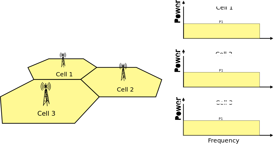
Full Frequency Reuse scheme
In ns-3, the NoOp FR algorithm always allows scheduler to use full bandwidth and allows all UEs to use any RBG. It simply does nothing new (i.e. it does not limit eNB bandwidth, FR algorithm is disabled), it is the simplest implementation of FrAlgorithm class and is installed in eNb by default.
Hard Frequency Reuse
The Hard Frequency Reuse algorithm provides the simplest scheme which allows to reduce inter-cell interference level. In this scheme whole frequency bandwidth is divided into few (typically 3, 4, or 7) disjoint sub-bands. Adjacent eNBs are allocated with different sub-band. Frequency reuse factor equals the number of sub-bands. This scheme allows to significantly reduce ICI at the cell edge, so the performance of cell-users is improved. But due to the fact, that each eNB uses only one part of whole bandwidth, peak data rate level is also reduced by the factor equal to the reuse factor.
Figure Hard Frequency Reuse scheme below presents frequency and power plan for Hard Frequency Reuse scheme.
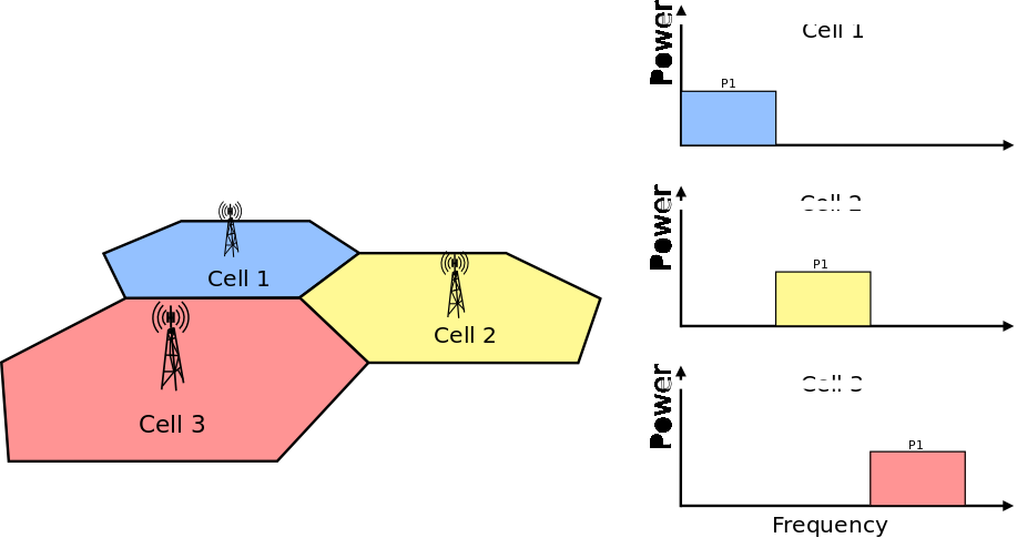
Hard Frequency Reuse scheme
In our implementation, the Hard FR algorithm has only vector of RBGs available for eNB and pass it to MAC Scheduler during scheduling functions. When scheduler ask, if RBG is allowed for specific UE it always return true.
Strict Frequency Reuse
Strict Frequency Reuse scheme is combination of Full and Hard Frequency Reuse schemes. It consists of dividing the system bandwidth into two parts which will have different frequency reuse. One common sub-band of the system bandwidth is used in each cell interior (frequency reuse-1), while the other part of the bandwidth is divided among the neighboring eNBs as in hard frequency reuse (frequency reuse-N, N>1), in order to create one sub-band with a low inter-cell interference level in each sector. Center UEs will be granted with the fully-reused frequency chunks, while cell-edge UEs with orthogonal chunks. It means that interior UEs from one cell do not share any spectrum with edge UEs from second cell, which reduces interference for both. As can be noticed, Strict FR requires a total of N + 1 sub-bands, and allows to achieve RFR in the middle between 1 and 3.
Figure Strict Frequency Reuse scheme below presents frequency and power plan for Strict Frequency Reuse scheme with a cell-edge reuse factor of N = 3.
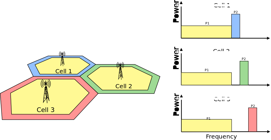
Strict Frequency Reuse scheme
In our implementation, Strict FR algorithm has two maps, one for each sub-band. If UE can be served within private sub-band, its RNTI is added to m_privateSubBandUe map. If UE can be served within common sub-band, its RNTI is added to m_commonSubBandUe map. Strict FR algorithm needs to decide within which sub-band UE should be served. It uses UE measurements provided by RRB and compare them with signal quality threshold (this parameter can be easily tuned by attribute mechanism). Threshold has influence on interior to cell radius ratio.
Soft Frequency Reuse
In Soft Frequency Reuse (SFR) scheme each eNb transmits over the entire system bandwidth, but there are two sub-bands, within UEs are served with different power level. Since cell-center UEs share the bandwidth with neighboring cells, they usually transmit at lower power level than the cell-edge UEs. SFR is more bandwidth efficient than Strict FR, because it uses entire system bandwidth, but it also results in more interference to both cell interior and edge users.
There are two possible versions of SFR scheme:
In first version, the sub-band dedicated for the cell-edge UEs may also be used by the cell-center UEs but with reduced power level and only if it is not occupied by the cell-edge UEs. Cell-center sub-band is available to the centre UEs only. Figure Soft Frequency Reuse scheme version 1 below presents frequency and power plan for this version of Soft Frequency Reuse scheme.
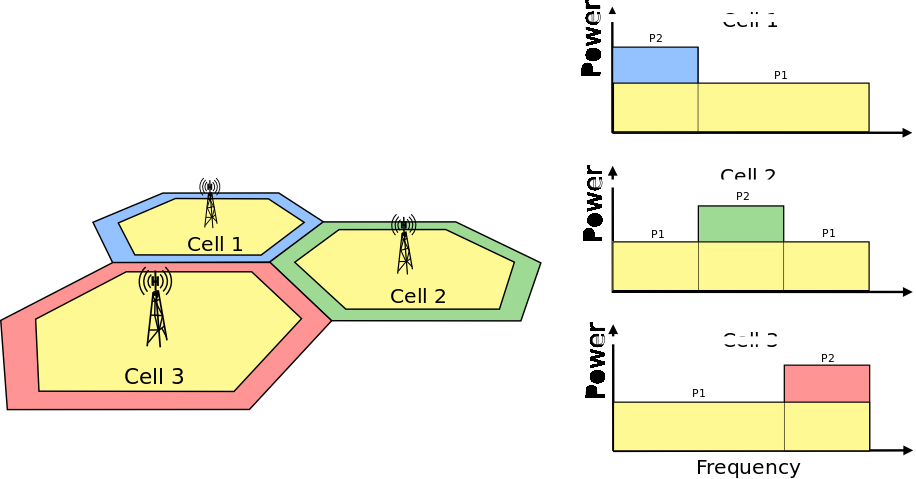
Soft Frequency Reuse scheme version 1
In second version, cell-center UEs do not have access to cell-edge sub-band. In this way, each cell can use the whole system bandwidth while reducing the interference to the neighbors cells. From the other hand, lower ICI level at the cell-edge is achieved at the expense of lower spectrum utilization. Figure Soft Frequency Reuse scheme version 2 below presents frequency and power plan for this version of Soft Frequency Reuse scheme.
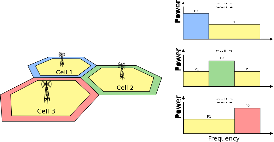
Soft Frequency Reuse scheme version 2
SFR algorithm maintain two maps. If UE should be served with lower power level, its RNTI is added to m_lowPowerSubBandUe map. If UE should be served with higher power level, its RNTI is added to m_highPowerSubBandUe map. To decide with which power level UE should be served SFR algorithm utilize UE measurements, and compares them to threshold. Signal quality threshold and PdschConfigDedicated (i.e. P_A value) for inner and outer area can be configured by attributes system. SFR utilizes Downlink Power Control described here.
Soft Fractional Frequency Reuse
Soft Fractional Frequency Reuse (SFFR) is an combination of Strict and Soft Frequency Reuse schemes. While Strict FR do not use the subbands allocated for outer region in the adjacent cells, soft FFR uses these subbands for the inner UEs with low transmit power. As a result, the SFFR, like SFR, use the subband with high transmit power level and with low transmit power level. Unlike the Soft FR and like Strict FR, the Soft FFR uses the common sub-band which can enhance the throughput of the inner users.
Figure Soft Fractional Fractional Frequency Reuse scheme below presents frequency and power plan for Soft Fractional Frequency Reuse.
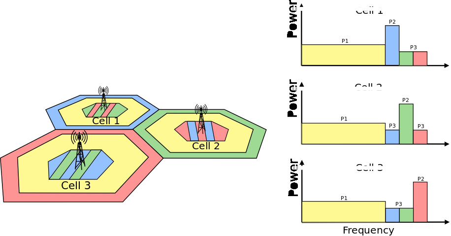
Soft Fractional Fractional Frequency Reuse scheme
Enhanced Fractional Frequency Reuse
Enhanced Fractional Frequency Reuse (EFFR) described in [ZXie2009] defines 3 cell-types for directly neighboring cells in a cellular system, and reserves for each cell-type a part of the whole frequency band named Primary Segment, which among different type cells should be orthogonal. The remaining subchannels constitute the Secondary Segment. The Primary Segment of a cell-type is at the same time a part of the Secondary Segments belonging to the other two cell-types. Each cell can occupy all subchannels of its Primary Segment at will, whereas only a part of subchannels in the Secondary Segment can be used by this cell in an interference-aware manner.The Primary Segment of each cell is divided into a reuse-3 part and reuse-1 part. The reuse-1 part can be reused by all types of cells in the system, whereas reuse-3 part can only be exclusively reused by other same type cells( i.e. the reuse-3 subchannels cannot be reused by directly neighboring cells). On the Secondary Segment cell acts as a guest, and occupying secondary subchannels is actually reuse the primary subchannels belonging to the directly neighboring cells, thus reuse on the Secondary Segment by each cell should conform to two rules:
- monitor before use
- resource reuse based on SINR estimation
Each cell listens on every secondary subchannel all the time. And before occupation, it makes SINR evaluation according to the gathered channel quality information (CQI) and chooses resources with best estimation values for reuse. If CQI value for RBG is above configured threshold for some user, transmission for this user can be performed using this RBG.
In [ZXie2009] scheduling process is described, it consist of three steps and two scheduling polices. Since none of currently implemented schedulers allow for this behaviour, some simplification were applied. In our implementation reuse-1 subchannels can be used only by cell center users. Reuse-3 subchannels can be used by edge users, and only if there is no edge user, transmission for cell center users can be served in reuse-3 subchannels.
Figure Enhanced Fractional Fractional Frequency Reuse scheme below presents frequency and power plan for Enhanced Fractional Frequency Reuse.
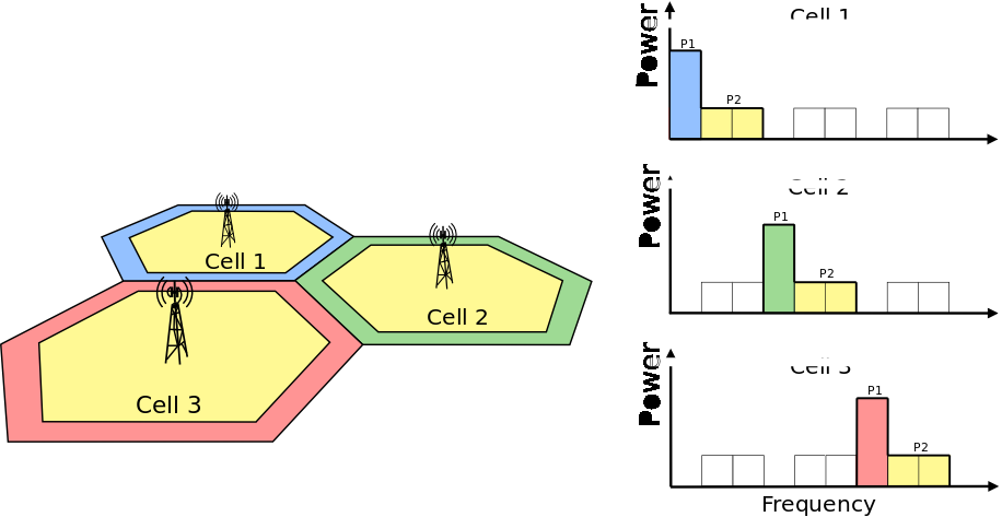
Enhanced Fractional Fractional Frequency Reuse scheme
Distributed Fractional Frequency Reuse
This Distributed Fractional Frequency Reuse Algorithm was presented in [DKimura2012]. It
automatically optimizes cell-edge sub-bands by focusing on user distribution (in particular,
receive-power distribution). This algorithm adaptively selects RBs for cell-edge sub-band on
basis of coordination information from adjecent cells and notifies the base stations of the
adjacent cells, which RBs it selected to use in edge sub-band. The base station of each cell
uses the received information and the following equation to compute cell-edge-band metric
 for each RB.
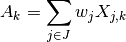
where  is a set of neighbor cells,
  is the RNTP from the -th
neighbor cell. It takes a value of 1 when the -th RB in the -th neighbor cell is used
as a cell-edge sub-band and 0 otherwise. The symbol
is the RNTP from the -th
neighbor cell. It takes a value of 1 when the -th RB in the -th neighbor cell is used
as a cell-edge sub-band and 0 otherwise. The symbol  denotes weight with respect to adjacent
cell , that is, the number of users for which the difference between the power of the signal
received from the serving cell and the power of the signal received from the adjacent cell
is less than a threshold value (i.e., the number of users near the cell edge in the service cell). A large
received power difference means that cell-edge users in the -th cell suffer strong interference
from the -th cell.
denotes weight with respect to adjacent
cell , that is, the number of users for which the difference between the power of the signal
received from the serving cell and the power of the signal received from the adjacent cell
is less than a threshold value (i.e., the number of users near the cell edge in the service cell). A large
received power difference means that cell-edge users in the -th cell suffer strong interference
from the -th cell.
The RB for which metric is smallest is considered to be least affected by interference from
another cell. Serving cell selects a configured number of RBs as cell-edge sub-band in ascending order
of . As a result, the RBs in which a small number of cell-edge users receive high
interference from adjacent base stations are selected.
The updated RNTP is then sent to all the neighbor cells. In order to avoid the meaningless oscillation of cell-edge-band selection, a base station ignores an RNTP from another base station that has larger cell ID than the base station.
Repeating this process across all cells enables the allocation of RBs to cell-edge areas to be optimized over the system and to be adjusted with changes in user distribution.
Figure Sequence diagram of Distributed Frequency Reuse Scheme below presents sequence diagram of Distributed Fractional Frequency Reuse Scheme.
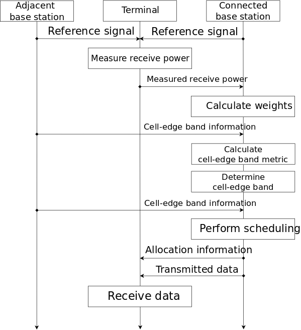
Sequence diagram of Distributed Frequency Reuse Scheme
Carrier Aggregation
Overview
This section describes the ns-3 support for Carrier Aggregation. The references in the standard are [TS36211], [TS36213] and [TS36331].
Note: Carrier Aggregation was introduced in release 3.27 and currently, only works in downlink.
3GPP standardizes, in release R10, the Carrier Aggregation (CA) technology.
This technology consists of the possibility, to aggregate radio resources belonging to different carriers, in order to have more bandwidth available, and to achieve a higher throughput. Carrier Aggregation as defined by 3GPP can be used with both TDD and FDD. Since ns-3 only supports FDD LTE implementation, we will consider only this case in this section. Each aggregated carrier is referred to as a component carrier, CC. The component carrier can have a bandwidth of 1.4, 3, 5, 10, 15 or 20 MHz and a maximum of five component carriers can be aggregated, hence the maximum aggregated bandwidth is 100 MHz. In FDD the number of aggregated carriers can be different in DL and UL. However, the number of UL component carriers is always equal to or lower than the number of DL component carriers. The individual component carriers can also be of different bandwidths. When carrier aggregation is used there are a number of serving cells, one for each component carrier. The coverage of the serving cells may differ, for example due to that CCs on different frequency bands will experience different pathloss. The RRC connection is only handled by one cell, the Primary serving cell, served by the Primary component carrier (DL and UL PCC). It is also on the DL PCC that the UE receives NAS information, such as security parameters.
3GPP defines three different CA bandwidth classes in releases 10 and 11 (where ATBC is Aggregated Transmission Bandwidth Configuration):
Class A: ATBC  100, maximum number of CC = 1
Class B: ATBC 100, maximum number of CC = 2
Class C: 100 ATBC 200, maximum number of CC = 2
Figure CA impact on different layers of LTE protocol stack (from 3gpp.org) (from 3gpp.org) shows the main impact of CA technology on the different layers of the LTE protocol stack. Introduction of carrier aggregation influences mainly the MAC and new RRC messages are introduced. In order to keep R8/R9 compatibility the protocol changes will be kept to a minimum. Basically each component carrier is treated as an R8 carrier. However some changes are required, such as new RRC messages in order to handle the secondary component carrier (SCC), and MAC must be able to handle scheduling on a number of CCs. In the following we describe the impact of the carrier aggregation implementation on the different layers of the LTE protocol stack in ns-3.
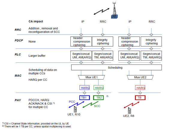
CA impact on different layers of LTE protocol stack (from 3gpp.org)
Impact on RRC layer
The main impacts on the RRC layer are related to secondary carrier configuration and measurements reporting. To enable these features we have enhanced the already existing procedures for the RRC Connection Reconfiguration and UE RRC Measurements Model.
The carrier aggregation enabling procedure is shown in figure A schematic overview of the secondary carrier enabling procedure.
As per 3GPP definition, the secondary cell is a cell, operating on a secondary frequency,
which may be configured once an RRC connection is established and which may be used to
provide additional radio resources. Hence, the procedure starts when the UE is in the
CONNECTED_NORMALLY state (see the RRC state machine description). This part of the procedure
is the same as in the previous architecture. In order to simplify the implementation,
the UE Capability Inquiry and UE Capability Information are not implemented. This
implies to assume that each UE can support the carrier aggregation, and any specific
configuration provided by the eNB to which is attached. The eNB RRC sends to the UE the
secondary carrier configuration parameters through the RRC Connection Reconfiguration
procedure. This procedure may be used for various purposes related to modifications of
the RRC connection, e.g. to establish, modify or release RBs, to perform handover, to
setup, modify or release measurements, to add, modify and release secondary cells (SCells).
At UE side, the RRC is extended to configure the lower layers, in such a way that the
SCell(s) are considered. Once the carriers are configured, the Reconfiguration Completed
message is sent back to the eNB RRC, informing the eNB RRC and CCM that the secondary
carriers have been properly configured. The RRC layer at both the UE and the eNB sides
is extended to allow measurement reporting for the secondary carriers. Finally, in order
to allow the procedures for configuration and measurement reporting, the RRC is enhanced
to support serialization and deserialization of RRC message structures that carry information
related to the secondary carriers, e.g., if the RRCConnectionReconfiguration message
includes sCellToAddModList structure, SCell addition or modification will be performed,
or, if it contains measConfig the measurement reporting will be configured. To allow
transmission of this information the following structures are implemented for the sCell:
RadioResourceConfigCommonSCell, RadioResourceConfigDedicatedSCell and
PhysicalConfigDedicatedSCell and NonCriticalExtensionConfiguration.
RadioResourceConfigCommonSCell and RadioResourceConfigDedicatedSCell are
used for SCell addition and modification (see TS 36.331, 5.3.10.3b).
PhysicalConfigDedicatedSCell is used for physical channel reconfiguration
(see TS 36.331, 5.3.10.6). Finally, NonCriticalExtensionConfiguration is used to
carry information of sCellToAddModeList and sCellToReleaseList,
which is a modified structure comparing to TS 36.331, 6.6.2, according to which these
are directly in the root of RRCConnectionReconfiguration message. Measurement
reporting is extended with measResultSCell structure to include RSRP and RSRQ
measurements for each configured SCell. However, the measurement report triggering
event A6 (neighbour becomes offset better than SCell) is not implemented yet.
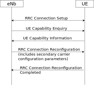
A schematic overview of the secondary carrier enabling procedure
Impact on PCDCP layer
There is no impact on PDCP layer.
Impact on RLC layer
The impact on the RLC layer is relatively small. There is some impact on configuration of
the buffer and the usage of SAP interfaces between RLC and MAC. Since the capacity of the
lower layers increases with the carrier aggregation it is necessary to accordingly adjust
the size of the RLC buffer. The impact on the implementation of the RLC layer is very small
thanks to the design choice that allows the CCM manager to serve the different RLC instances
through the LteMacSapProvider interface. Thanks to this design choice, the RLC is using
the same interface as in the earlier LTE module architecture, the LteMacSapProvider,
but the actual SAP provider in the new architecture is the CCM (some class that inherits
LteEnbComponentCarrierManager). The CCM acts as a proxy, it receives function calls
that are meant for the MAC, and forwards them to the MAC of the different component
carriers. Additionally, it uses the information of the UEs and the logical channels for
its own functionalities.
Impact on MAC layer
The impact on the MAC layer depends on the CA scheduling scheme in use. Two different scheduling schemes are proposed in R10 and are shown in figure CA scheduling schemes (from 3gpp.org).
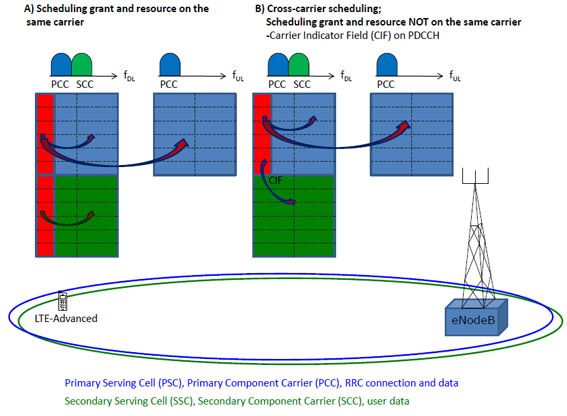
CA scheduling schemes (from 3gpp.org)
The CIF (Carrier Indicator Field) on PDCCH (represented by the red area) indicates on which carrier the scheduled resource is located. In the following we describe both the schemes:
- scheduling grant and resources on the same carrier. One PDCCH is supported per carrier.
- cross-carrier scheduling: it is used to schedule resources on the secondary carrier without PDCCH.
Current implementation covers only option 1, so there is no cross-carrier scheduling. The MAC layer of the eNodeB has suffered minor changes and they are mainly related to addition of component carrier information in message exchange between layers.
Impact on PHY layer
The impact on PHY layer is minor. There is an instance of PHY layer per each component carrier and the SAP interface functions remain unchanged. As shown in CA scheduling schemes (from 3gpp.org) the difference is that since there are multiple PHY instances, there are also multiple instances of PDCCH, HARQ, ACK/NACK and CSI per carrier. So, at the eNB PHY, the changes are related to the addition of the component carrier id information, while at the UE PHY the information of the Component Carrier is used for some functionalities that depend on the Component Carrier to which the PHY instance belongs. For example, the UE PHY is extended to allow disabling of the sounding reference signal (SRS) at the secondary carriers. This is necessary because there is one UE PHY instance per component carrier, but according to CA scheduling schemes (from 3gpp.org), only a single carrier is used and the uplink traffic is transmitted only over the primary carrier.
Code Structure Design
This section briefly introduces the software design and implementation of the carrier aggregation functionality.
Both LteEnbNetDevice and LteUeNetDevice are created by the LteHelper
using the method InstallSingleEnbDevice and InstallSingleUeDevice. These
functions are now extended to allow the carrier aggregation configuration. In the
following we explain the main differences comparing to the previous architecture.
Figure Changes in LteEnbNetDevice to support CA shows the attributes and associations
of the LteEnbNetDevice that are affected by the implementation, or are created
in order to support the carrier aggregation functionality. Since LteEnbNetDevice
may have several component carriers, the attributes that were formerly part of
the LteEnbNetDevice and are carrier specific are migrated to the ComponentCarrier
class, e.g. physical layer configuration parameters. The attributes that are
specific for the eNB component carrier are migrated to ComponentCarrierEnb, e.g.
pointers to MAC, PHY, scheduler, fractional frequency reuse instances.
LteEnbNetDevice can contain pointers to several ComponentCarrierEnb instances.
This architecture allows that each CC may have its own configuration for PHY, MAC,
scheduling algorithm and franctional frequency reuse algorithm. These attributes are
currently maintained also in the LteEnbNetDevice for backward compatibility purpose.
By default the LteEnbNetDevice attributes are the same as the
primary carrier attributes.
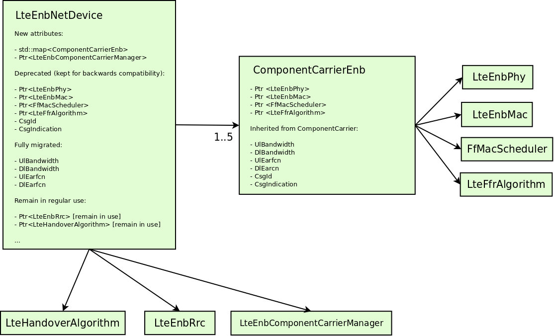
Changes in LteEnbNetDevice to support CA
Figure Changes in LteUeNetDevice to support CA shows the attributes and associations
of LteUeNetDevice that are affected by the carrier aggregation implementation.
Similarly, to the changes in LteEnbNetDevice, pointers that are specific to UE
component carrier are migrated to the ComponentCarrierUe class.
LteUeNetDevice has maintained m_dlEarfcn for initial cell selection purposes.
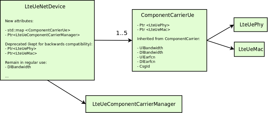
Changes in LteUeNetDevice to support CA
CA impact on data plane of eNodeB
Figure eNB Data Plane Architecture shows the class diagram of the data plane at the eNB.
The main impact is the insertion of the LteEnbComponentCarrierManager class
in the middle of the LTE protocol stack. During the design phase it was
decided to keep the same SAP interfaces design that existed between MAC and RLC
in order to avoid unnecessary changes in these parts of protocol stack.
To achieve this the LteEnbComponentCarrierManager implements all functions
that were previously exposed by RLC to MAC through LteMacSapUser interface.
It also implements functions that were previously exposed by MAC to RLC through
the LteMacSapProvider interface. In this way, the carrier aggregation is
transparent to upper and lower layers. The only difference is that the MAC
instance sees now only one LteMacSapUser, whereas formerly it was seeing only
one LteMacSapUser per RLC instance.
The LteEnbComponentCarrierManager is responsible for the forwarding messages
in both directions. In the current implementation, a PDCP and a RLC instances are
activated each time a new data radio bearer is configured. The correspondence
between a new data radio bearer and a RLC instance is one to one. In order to
maintain the same behavior, when a new logical channel is activated, the logical
channel configurations is propagated to each MAC layer object in “as is” fashion.
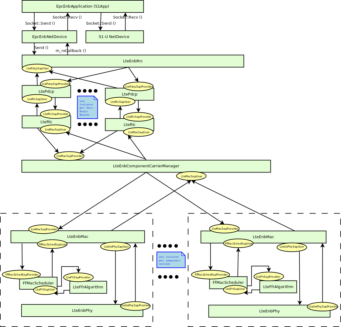
eNB Data Plane Architecture
Figure Sequence Diagram of downlink buffer status reporting (BSR) with CA shows a sequence diagram of downlink buffer status
reporting with a carrier aggregation implementation of only one secondary carrier.
Each time that an RLC instance sends a buffer status report (BSR), the
LteEnbComponentCarrierManager propagates the BSR to the MAC instances.
The LteEnbComponentCarrierManager may modify a BSR before sending it to the
MAC instances. This modification depends on the traffic split algorithm implemented
in CCM class that inherits LteEnbComponentCarrierManager.
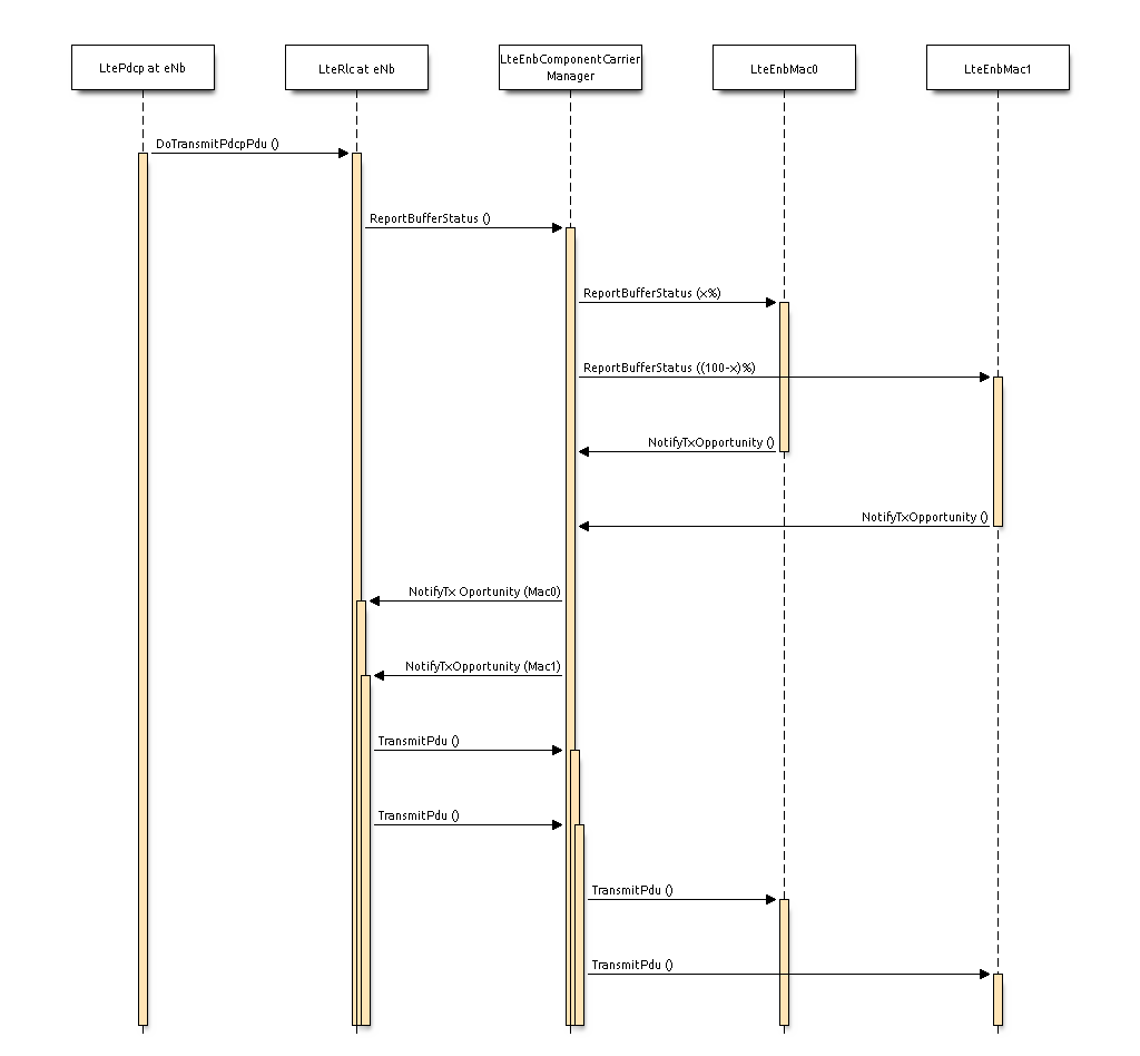
Sequence Diagram of downlink buffer status reporting (BSR) with CA
CA impact on control plane of eNodeB
Figure eNB Control Plane Architecture shows the class diagram of the control plane
at the eNB. During the design phase it was decided to maintain the same hooks as in
the former architecture. To do so, at each component carrier the PHY and the MAC are
directly associated to the RRC instance. However, the RRC instance is additionally
connected to the LteEnbComponentCarrierManager, which is responsible for enabling
and disabling the component carriers. When the simulation starts, the number of
component carrier is fixed, but only the primary carrier component is enabled.
Depending on the LteEnbComponentCarrierManager algorithm the other carrier
components could be activated or not.
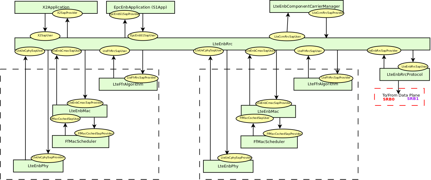
eNB Control Plane Architecture
Figure Sequence Diagram of Data Radio Bearer Setup shows how the Radio Bearer are configured.
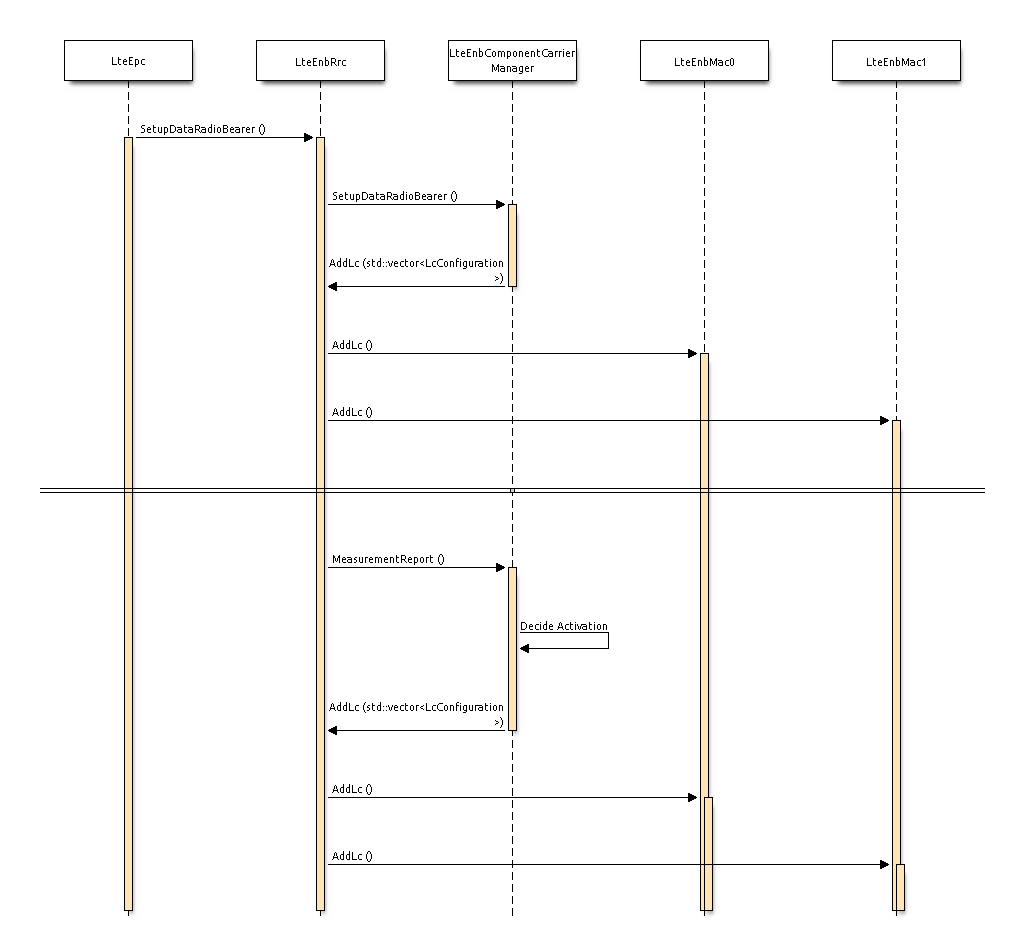
Sequence Diagram of Data Radio Bearer Setup
CA impact on data plane of UE
Figure UE Data Plane Architecture shows the relation between the different classes
related to the UE data plane. The UE data plane architecture is similar to the eNB data
plane implementation. The LteUeComponentCarrierManager is responsible to (re)map
each MacSapUserProvider to the corresponding RLC instance or to the proper MAC
instance. The channel remapping depends on algorithm used as LteUeComponentCarrierManager.
A particular case is represented by the UE buffer status report (BSR) to eNB.
Since, i) the standard does not specify how the BSR has to be reported on each component
carrier and ii) it is decided to map one-to-one the logical channel to each MAC layer,
the only way to send BSRs to the eNB is through the primary carrier.
Figure Uplink buffer status reporting with CA shows the sequence diagram.
Each time a BSR is generated, the LteUeComponentCarrierManager sends it through
the primary carrier component. When the primary component carrier at the eNB receives
the BSR, it sends it to LteEnbComponentCarrierManager. The latter, according to
algorithm dependent policies, forwards a BSR to component carriers. The communication
between the LteEnbMac and the LteEnbComponentCarrierManager is done through a
specific set of SAP functions which are implemented in the LteUlCcmRrcSapUser and
the LteUlCcmRrcSapProvider.
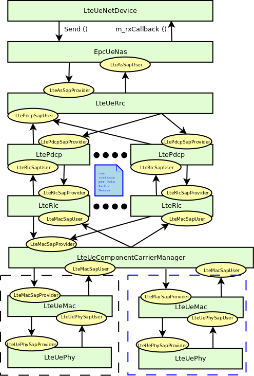
UE Data Plane Architecture
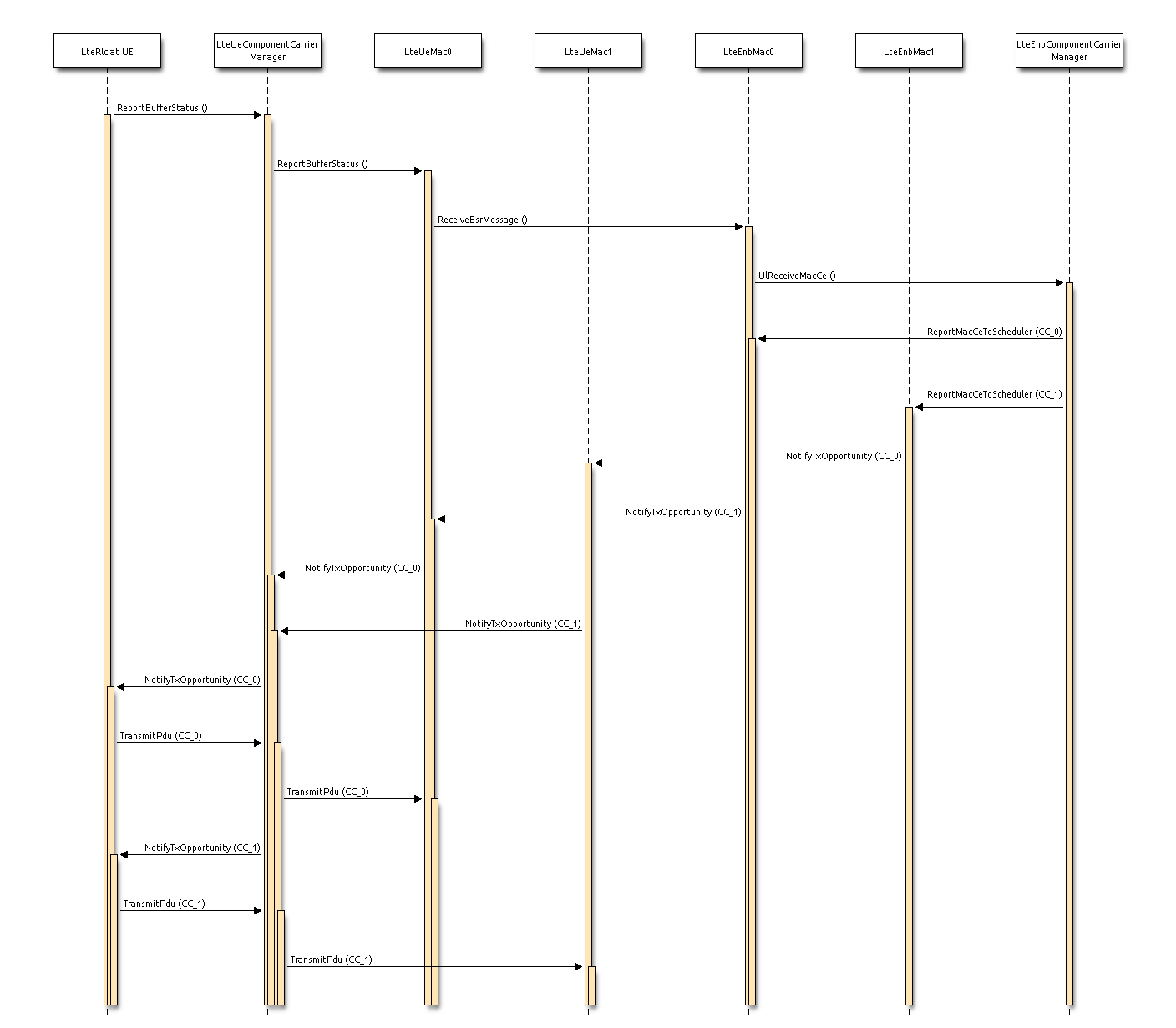
Uplink buffer status reporting with CA
CA impact on control plane of UE
Figure UE Control Plane Architecture shows the relation between the different classes
associated to the UE control plane. The control plane implementation at the UE is basically
the same as the eNB control plane implementation. Each component carrier control SAP
(both for PHY and MAC layer objects) is linked in a one-to-one fashion directly to the RRC
instance. The Ue RRC instance is then connected to the LteUeComponentCarrierManager
in the same way as in the eNB.
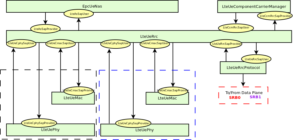
UE Control Plane Architecture
CCHelper is the class that is implemented to help the configuration of the physical
layer parameters, such as uplink and downlink,bandwidth and EARFCN of each carrier.
CCM RRC MAC interfaces
The Component carrier manager (CCM) is also developed by using the SAP interface design. The following SAP interfaces are implemented for CCM and MAC:
- the
LteCcmMacSapUserpart is provided by MAC and is used by the CCM- the
LteCcmMacSapProviderpart is provided by CCM and is used by the MAC layerWhen the primary component carrier receives an uplink BSR it uses the
LteCcmMacSapUserto forward it to the CCM, which should decide how to split the traffic corresponding to this BSR among carriers. Once this decision is made, the CCM uses theLteCcmMacSapProviderinterface to send back an uplink BSR to some of the MAC instances. Additionally, theLteCcmMacSapUsercan be used by the MAC to notify about the PRB occupancy in the downlink to the CCM. This information may be used by the CCM to decide how to split the traffic and whether to use the secondary carriers.
CCM RRC SAP interfaces
The following SAP interfaces are implemented for CCM and RRC:
- the
LteCcmRrcSapProvideris provided by the CCM and is used by the RRC layer- the
LteCcmRrcSapUseris provided by RRC and is used by the CCM
By using the LteCcmRrcSapUser the CCM may request a specific measurement reporting
configuration to be fulfilled by the UEs attached to the eNB. When a UE measurement
report is received, as a result of this configuration, the eNB RRC entity shall forward
this report to the CCM through the LteCcmRrcSapProvider::ReportUeMeas SAP function.
Additionally, the LteCcmRrcSapProvider offers different functions to the RRC that can
be used to add and remove of UEs, setup or release of radio bearer, configuration of the
signalling bearer, etc.
Component carrier managers
Currently, there are two component carrier manager implementations available. The first one
is the NoOpComponentCarrierManager, which is the default CCM choice. When this CCM is
used the carrier aggregation feature is disabled. This CCM forwards all traffic, the uplink
and the downlink, over
the primary carrier, and does not use secondary carriers.
Another implementation is the RrComponentCarrierManager, which splits the traffic
equally among carriers, by diving the buffer status report among different carriers.
SRB0 and SRB1 flows will be forwarded only over primary carrier.
Helpers
Two helper objects are used to setup simulations and configure the various components. These objects are:
LteHelper, which takes care of the configuration of the LTE radio access network, as well as of coordinating the setup and release of EPS bearers. TheLteHelperclass provides both the API definition and its implementation.EpcHelper, which takes care of the configuration of the Evolved Packet Core. TheEpcHelperclass is an abstract base class, which only provides the API definition; the implementation is delegated to the child classes in order to allow for different EPC network models.
A third helper object is used to configure the Carrier Aggregation functionality:
CcHelper, which takes care of the configuration of theLteEnbComponentCarrierMap, basically, it creates a user specified number ofLteEnbComponentCarrier.LteUeComponentCarrierMapis currently created starting from theLteEnbComponentCarrierMap.LteHelper:InstallSingleUeDevice, in this implementation, is needed to invoke after theLteHelper:InstallSingleEnbDeviceto ensure that theLteEnbComponentCarrierMapis properly initialized.
It is possible to create a simple LTE-only simulations by
using the LteHelper alone, or to create complete LTE-EPC simulations by using both
LteHelper and EpcHelper. When both helpers are used, they interact in a master-slave
fashion, with the LteHelper being the Master that interacts directly with the user program,
and the EpcHelper working “under the hood” to configure the EPC upon explicit methods
called by the LteHelper. The exact interactions are displayed in the Figure Sequence diagram of the interaction between LteHelper and EpcHelper..
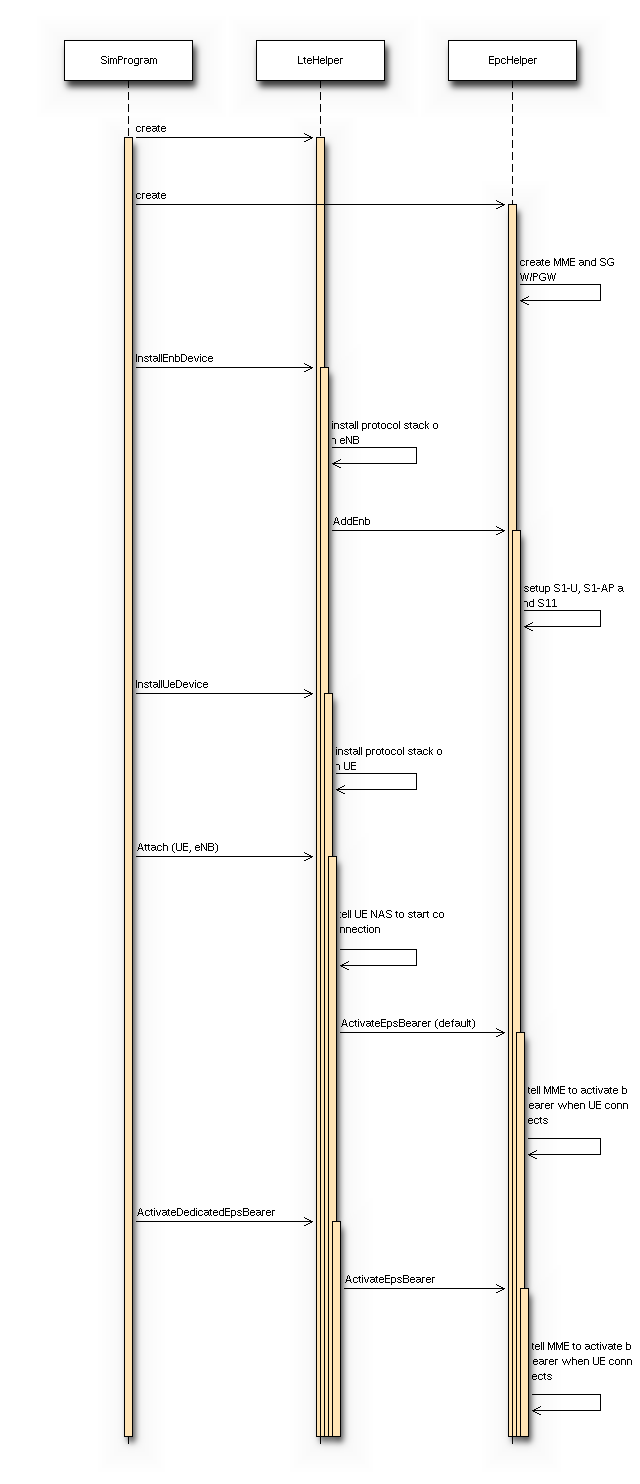
Sequence diagram of the interaction between LteHelper and EpcHelper.
User Documentation
Background
We assume the reader is already familiar with how to use the ns-3 simulator to run generic simulation programs. If this is not the case, we strongly recommend the reader to consult [ns3tutorial].
Usage Overview
The ns-3 LTE model is a software library that allows the simulation of LTE networks, optionally including the Evolved Packet Core (EPC). The process of performing such simulations typically involves the following steps:
- Define the scenario to be simulated
- Write a simulation program that recreates the desired scenario topology/architecture. This is done accessing the ns-3 LTE model library using the
ns3::LteHelperAPI defined insrc/lte/helper/lte-helper.h.- Specify configuration parameters of the objects that are being used for the simulation. This can be done using input files (via the
ns3::ConfigStore) or directly within the simulation program.- Configure the desired output to be produced by the simulator
- Run the simulation.
All these aspects will be explained in the following sections by means of practical examples.
Basic simulation program
Here is the minimal simulation program that is needed to do an LTE-only simulation (without EPC).
Initial boilerplate:
#include <ns3/core-module.h>
#include <ns3/network-module.h>
#include <ns3/mobility-module.h>
#include <ns3/lte-module.h>

using namespace ns3;

int main (int argc, char *argv[])
{
  // the rest of the simulation program follows
Create an
LteHelperobject:Ptr<LteHelper> lteHelper = CreateObject<LteHelper> ();
This will instantiate some common objects (e.g., the Channel object) and provide the methods to add eNBs and UEs and configure them.
Create
Nodeobjects for the eNB(s) and the UEs:NodeContainer enbNodes; enbNodes.Create (1); NodeContainer ueNodes; ueNodes.Create (2);
Note that the above Node instances at this point still don’t have an LTE protocol stack installed; they’re just empty nodes.
Configure the Mobility model for all the nodes:
MobilityHelper mobility;
mobility.SetMobilityModel ("ns3::ConstantPositionMobilityModel");
mobility.Install (enbNodes);
mobility.SetMobilityModel ("ns3::ConstantPositionMobilityModel");
mobility.Install (ueNodes);
The above will place all nodes at the coordinates (0,0,0). Please refer to the documentation of the ns-3 mobility model for how to set your own position or configure node movement.
Install an LTE protocol stack on the eNB(s):
NetDeviceContainer enbDevs;
enbDevs = lteHelper->InstallEnbDevice (enbNodes);
Install an LTE protocol stack on the UEs:
NetDeviceContainer ueDevs;
ueDevs = lteHelper->InstallUeDevice (ueNodes);
Attach the UEs to an eNB. This will configure each UE according to the eNB configuration, and create an RRC connection between them:
lteHelper->Attach (ueDevs, enbDevs.Get (0));
Activate a data radio bearer between each UE and the eNB it is attached to:
enum EpsBearer::Qci q = EpsBearer::GBR_CONV_VOICE;
EpsBearer bearer (q);
lteHelper->ActivateDataRadioBearer (ueDevs, bearer);
this method will also activate two saturation traffic generators for that bearer, one in uplink and one in downlink.
Set the stop time:
Simulator::Stop (Seconds (0.005));
This is needed otherwise the simulation will last forever, because (among others) the start-of-subframe event is scheduled repeatedly, and the ns-3 simulator scheduler will hence never run out of events.
Run the simulation:
Simulator::Run ();
Cleanup and exit:
Simulator::Destroy ();
return 0;
}
For how to compile and run simulation programs, please refer to [ns3tutorial].
Configuration of LTE model parameters
All the relevant LTE model parameters are managed through the ns-3 attribute system. Please refer to the [ns3tutorial] and [ns3manual] for detailed information on all the possible methods to do it (environmental variables, C++ API, GtkConfigStore…).
In the following, we just briefly summarize
how to do it using input files together with the ns-3 ConfigStore.
First of all, you need to put the following in your simulation
program, right after main () starts:
CommandLine cmd (__FILE__);
cmd.Parse (argc, argv);
ConfigStore inputConfig;
inputConfig.ConfigureDefaults ();
// parse again so you can override default values from the command line
cmd.Parse (argc, argv);
for the above to work, make sure you also #include "ns3/config-store.h".
Now create a text file named (for example) input-defaults.txt
specifying the new default values that you want to use for some attributes:
default ns3::LteHelper::Scheduler "ns3::PfFfMacScheduler"
default ns3::LteHelper::PathlossModel "ns3::FriisSpectrumPropagationLossModel"
default ns3::LteEnbNetDevice::UlBandwidth "25"
default ns3::LteEnbNetDevice::DlBandwidth "25"
default ns3::LteEnbNetDevice::DlEarfcn "100"
default ns3::LteEnbNetDevice::UlEarfcn "18100"
default ns3::LteUePhy::TxPower "10"
default ns3::LteUePhy::NoiseFigure "9"
default ns3::LteEnbPhy::TxPower "30"
default ns3::LteEnbPhy::NoiseFigure "5"
Supposing your simulation program is called
src/lte/examples/lte-sim-with-input, you can now pass these
settings to the simulation program in the following way:
./waf --command-template="%s --ns3::ConfigStore::Filename=input-defaults.txt
--ns3::ConfigStore::Mode=Load --ns3::ConfigStore::FileFormat=RawText"
--run src/lte/examples/lte-sim-with-input
Furthermore, you can generate a template input file with the following command:
./waf --command-template="%s --ns3::ConfigStore::Filename=input-defaults.txt
--ns3::ConfigStore::Mode=Save --ns3::ConfigStore::FileFormat=RawText"
--run src/lte/examples/lte-sim-with-input
note that the above will put in the file input-defaults.txt all
the default values that are registered in your particular build of the
simulator, including lots of non-LTE attributes.
Configure LTE MAC Scheduler
There are several types of LTE MAC scheduler user can choose here. User can use following codes to define scheduler type:
Ptr<LteHelper> lteHelper = CreateObject<LteHelper> ();
lteHelper->SetSchedulerType ("ns3::FdMtFfMacScheduler");    // FD-MT scheduler
lteHelper->SetSchedulerType ("ns3::TdMtFfMacScheduler");    // TD-MT scheduler
lteHelper->SetSchedulerType ("ns3::TtaFfMacScheduler");     // TTA scheduler
lteHelper->SetSchedulerType ("ns3::FdBetFfMacScheduler");   // FD-BET scheduler
lteHelper->SetSchedulerType ("ns3::TdBetFfMacScheduler");   // TD-BET scheduler
lteHelper->SetSchedulerType ("ns3::FdTbfqFfMacScheduler");  // FD-TBFQ scheduler
lteHelper->SetSchedulerType ("ns3::TdTbfqFfMacScheduler");  // TD-TBFQ scheduler
lteHelper->SetSchedulerType ("ns3::PssFfMacScheduler");     //PSS scheduler
TBFQ and PSS have more parameters than other schedulers. Users can define those parameters in following way:
* TBFQ scheduler::

 Ptr<LteHelper> lteHelper = CreateObject<LteHelper> ();
 lteHelper->SetSchedulerAttribute("DebtLimit", IntegerValue(yourvalue)); // default value -625000 bytes (-5Mb)
 lteHelper->SetSchedulerAttribute("CreditLimit", UintegerValue(yourvalue)); // default value 625000 bytes (5Mb)
 lteHelper->SetSchedulerAttribute("TokenPoolSize", UintegerValue(yourvalue)); // default value 1 byte
 lteHelper->SetSchedulerAttribute("CreditableThreshold", UintegerValue(yourvalue)); // default value 0

* PSS scheduler::

 Ptr<LteHelper> lteHelper = CreateObject<LteHelper> ();
 lteHelper->SetSchedulerAttribute("nMux", UIntegerValue(yourvalue)); // the maximum number of UE selected by TD scheduler
 lteHelper->SetSchedulerAttribute("PssFdSchedulerType", StringValue("CoItA")); // PF scheduler type in PSS
In TBFQ, default values of debt limit and credit limit are set to -5Mb and 5Mb respectively based on paper [FABokhari2009].
Current implementation does not consider credit threshold ( = 0). In PSS, if user does not define nMux,
PSS will set this value to half of total UE. The default FD scheduler is PFsch.
In addition, token generation rate in TBFQ and target bit rate in PSS need to be configured by Guarantee Bit Rate (GBR) or Maximum Bit Rate (MBR) in epc bearer QoS parameters. Users can use following codes to define GBR and MBR in both downlink and uplink:
Ptr<LteHelper> lteHelper = CreateObject<LteHelper> ();
enum EpsBearer::Qci q = EpsBearer::yourvalue;  // define Qci type
GbrQosInformation qos;
qos.gbrDl = yourvalue; // Downlink GBR
qos.gbrUl = yourvalue; // Uplink GBR
qos.mbrDl = yourvalue; // Downlink MBR
qos.mbrUl = yourvalue; // Uplink MBR
EpsBearer bearer (q, qos);
lteHelper->ActivateDedicatedEpsBearer (ueDevs, bearer, EpcTft::Default ());
In PSS, TBR is obtained from GBR in bearer level QoS parameters. In TBFQ, token generation rate is obtained from the MBR setting in bearer level QoS parameters, which therefore needs to be configured consistently. For constant bit rate (CBR) traffic, it is suggested to set MBR to GBR. For variance bit rate (VBR) traffic, it is suggested to set MBR k times larger than GBR in order to cover the peak traffic rate. In current implementation, k is set to three based on paper [FABokhari2009]. In addition, current version of TBFQ does not consider RLC header and PDCP header length in MBR and GBR. Another parameter in TBFQ is packet arrival rate. This parameter is calculated within scheduler and equals to the past average throughput which is used in PF scheduler.
Many useful attributes of the LTE-EPC model will be described in the
following subsections. Still, there are many attributes which are not
explicitly mentioned in the design or user documentation, but which
are clearly documented using the ns-3 attribute system. You can easily
print a list of the attributes of a given object together with their
description and default value passing --PrintAttributes= to a simulation
program, like this:
./waf --run lena-simple --command-template="%s --PrintAttributes=ns3::LteHelper"
You can try also with other LTE and EPC objects, like this:
./waf --run lena-simple --command-template="%s --PrintAttributes=ns3::LteEnbNetDevice"
./waf --run lena-simple --command-template="%s --PrintAttributes=ns3::LteEnbMac"
./waf --run lena-simple --command-template="%s --PrintAttributes=ns3::LteEnbPhy"
./waf --run lena-simple --command-template="%s --PrintAttributes=ns3::LteUePhy"
./waf --run lena-simple --command-template="%s --PrintAttributes=ns3::PointToPointEpcHelper"
Simulation Output
The ns-3 LTE model currently supports the output to file of PHY, MAC, RLC and PDCP level Key Performance Indicators (KPIs). You can enable it in the following way:
Ptr<LteHelper> lteHelper = CreateObject<LteHelper> ();

// configure all the simulation scenario here...

lteHelper->EnablePhyTraces ();
lteHelper->EnableMacTraces ();
lteHelper->EnableRlcTraces ();
lteHelper->EnablePdcpTraces ();

Simulator::Run ();
RLC and PDCP KPIs are calculated over a time interval and stored on ASCII
files, two for RLC KPIs and two for PDCP KPIs, in each case one for
uplink and one for downlink. The time interval duration can be controlled using the attribute
ns3::RadioBearerStatsCalculator::EpochDuration.
The columns of the RLC KPI files is the following (the same for uplink and downlink):
- start time of measurement interval in seconds since the start of simulation
- end time of measurement interval in seconds since the start of simulation
- Cell ID
- unique UE ID (IMSI)
- cell-specific UE ID (RNTI)
- Logical Channel ID
- Number of transmitted RLC PDUs
- Total bytes transmitted.
- Number of received RLC PDUs
- Total bytes received
- Average RLC PDU delay in seconds
- Standard deviation of the RLC PDU delay
- Minimum value of the RLC PDU delay
- Maximum value of the RLC PDU delay
- Average RLC PDU size, in bytes
- Standard deviation of the RLC PDU size
- Minimum RLC PDU size
- Maximum RLC PDU size
Similarly, the columns of the PDCP KPI files is the following (again, the same for uplink and downlink):
- start time of measurement interval in seconds since the start of simulation
- end time of measurement interval in seconds since the start of simulation
- Cell ID
- unique UE ID (IMSI)
- cell-specific UE ID (RNTI)
- Logical Channel ID
- Number of transmitted PDCP PDUs
- Total bytes transmitted.
- Number of received PDCP PDUs
- Total bytes received
- Average PDCP PDU delay in seconds
- Standard deviation of the PDCP PDU delay
- Minimum value of the PDCP PDU delay
- Maximum value of the PDCP PDU delay
- Average PDCP PDU size, in bytes
- Standard deviation of the PDCP PDU size
- Minimum PDCP PDU size
- Maximum PDCP PDU size
Note: The PDCP traces for data radio bearers are not generated when SM RLC is used.
MAC KPIs are basically a trace of the resource allocation reported by the scheduler upon the start of every subframe. They are stored in ASCII files. For downlink MAC KPIs the format is the following:
- Simulation time in seconds at which the allocation is indicated by the scheduler
- Cell ID
- unique UE ID (IMSI)
- Frame number
- Subframe number
- cell-specific UE ID (RNTI)
- MCS of TB 1
- size of TB 1
- MCS of TB 2 (0 if not present)
- size of TB 2 (0 if not present)
while for uplink MAC KPIs the format is:
- Simulation time in seconds at which the allocation is indicated by the scheduler
- Cell ID
- unique UE ID (IMSI)
- Frame number
- Subframe number
- cell-specific UE ID (RNTI)
- MCS of TB
- size of TB
The names of the files used for MAC KPI output can be customized via
the ns-3 attributes ns3::MacStatsCalculator::DlOutputFilename and
ns3::MacStatsCalculator::UlOutputFilename.
PHY KPIs are distributed in seven different files, configurable through the attributes
ns3::PhyStatsCalculator::DlRsrpSinrFilenamens3::PhyStatsCalculator::UeSinrFilenamens3::PhyStatsCalculator::InterferenceFilenamens3::PhyStatsCalculator::DlTxOutputFilenamens3::PhyStatsCalculator::UlTxOutputFilenamens3::PhyStatsCalculator::DlRxOutputFilenamens3::PhyStatsCalculator::UlRxOutputFilename
In the RSRP/SINR file, the following content is available:
- Simulation time in seconds at which the allocation is indicated by the scheduler
- Cell ID
- unique UE ID (IMSI)
- RSRP
- Linear average over all RBs of the downlink SINR in linear units
The contents in the UE SINR file are:
- Simulation time in seconds at which the allocation is indicated by the scheduler
- Cell ID
- unique UE ID (IMSI)
- uplink SINR in linear units for the UE
In the interference filename the content is:
- Simulation time in seconds at which the allocation is indicated by the scheduler
- Cell ID
- List of interference values per RB
In UL and DL transmission files the parameters included are:
- Simulation time in milliseconds
- Cell ID
- unique UE ID (IMSI)
- RNTI
- Layer of transmission
- MCS
- size of the TB
- Redundancy version
- New Data Indicator flag
And finally, in UL and DL reception files the parameters included are:
- Simulation time in milliseconds
- Cell ID
- unique UE ID (IMSI)
- RNTI
- Transmission Mode
- Layer of transmission
- MCS
- size of the TB
- Redundancy version
- New Data Indicator flag
- Correctness in the reception of the TB
Note: The traces generated by simulating the scenarios involving the RLF will have a discontinuity in time from the moment of the RLF event until the UE connects again to an eNB.
Fading Trace Usage
In this section we will describe how to use fading traces within LTE simulations.
Fading Traces Generation
It is possible to generate fading traces by using a dedicated matlab script provided with the code (/lte/model/fading-traces/fading-trace-generator.m). This script already includes the typical taps configurations for three 3GPP scenarios (i.e., pedestrian, vehicular and urban as defined in Annex B.2 of [TS36104]); however users can also introduce their specific configurations. The list of the configurable parameters is provided in the following:
fc: the frequency in use (it affects the computation of the doppler speed).v_km_h: the speed of the userstraceDuration: the duration in seconds of the total length of the trace.numRBs: the number of the resource block to be evaluated.tag: the tag to be applied to the file generated.
The file generated contains ASCII-formatted real values organized in a matrix fashion: every row corresponds to a different RB, and every column correspond to a different temporal fading trace sample.
It has to be noted that the ns-3 LTE module is able to work with any fading trace file that complies with the above described ASCII format. Hence, other external tools can be used to generate custom fading traces, such as for example other simulators or experimental devices.
Fading Traces Usage
When using a fading trace, it is of paramount importance to specify correctly the trace parameters in the simulation, so that the fading model can load and use it correctly. The parameters to be configured are:
TraceFilename: the name of the trace to be loaded (absolute path, or relative path w.r.t. the path from where the simulation program is executed);TraceLength: the trace duration in seconds;SamplesNum: the number of samples;WindowSize: the size of the fading sampling window in seconds;
It is important to highlight that the sampling interval of the fading trace has to be 1 ms or greater, and in the latter case it has to be an integer multiple of 1 ms in order to be correctly processed by the fading module.
The default configuration of the matlab script provides a trace 10 seconds long, made of 10,000 samples (i.e., 1 sample per TTI=1ms) and used with a windows size of 0.5 seconds amplitude. These are also the default values of the parameters above used in the simulator; therefore their settage can be avoided in case the fading trace respects them.
In order to activate the fading module (which is not active by default) the following code should be included in the simulation program:
Ptr<LteHelper> lteHelper = CreateObject<LteHelper> ();
lteHelper->SetFadingModel("ns3::TraceFadingLossModel");
And for setting the parameters:
lteHelper->SetFadingModelAttribute ("TraceFilename", StringValue ("src/lte/model/fading-traces/fading_trace_EPA_3kmph.fad"));
lteHelper->SetFadingModelAttribute ("TraceLength", TimeValue (Seconds (10.0)));
lteHelper->SetFadingModelAttribute ("SamplesNum", UintegerValue (10000));
lteHelper->SetFadingModelAttribute ("WindowSize", TimeValue (Seconds (0.5)));
lteHelper->SetFadingModelAttribute ("RbNum", UintegerValue (100));
It has to be noted that, TraceFilename does not have a default value, therefore is has to be always set explicitly.
The simulator provide natively three fading traces generated according to the configurations defined in in Annex B.2 of [TS36104]. These traces are available in the folder src/lte/model/fading-traces/). An excerpt from these traces is represented in the following figures.

Excerpt of the fading trace included in the simulator for a pedestrian scenario (speed of 3 kmph).
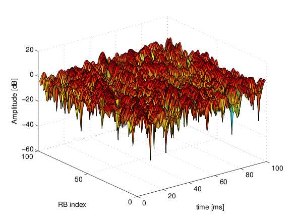
Excerpt of the fading trace included in the simulator for a vehicular scenario (speed of 60 kmph).
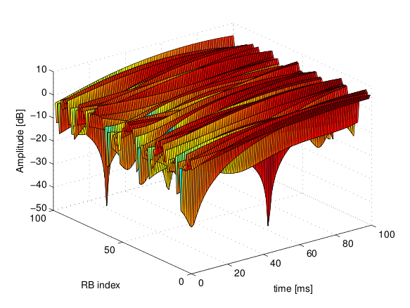
Excerpt of the fading trace included in the simulator for an urban scenario (speed of 3 kmph).
Mobility Model with Buildings
We now explain by examples how to use the buildings model (in particular, the MobilityBuildingInfo and the BuildingPropagationModel classes) in an ns-3 simulation program to setup an LTE simulation scenario that includes buildings and indoor nodes.
Header files to be included:
#include <ns3/mobility-building-info.h>
#include <ns3/buildings-propagation-loss-model.h>
#include <ns3/building.h>
Pathloss model selection:
Ptr<LteHelper> lteHelper = CreateObject<LteHelper> ();

lteHelper->SetAttribute ("PathlossModel", StringValue ("ns3::BuildingsPropagationLossModel"));
EUTRA Band Selection
The selection of the working frequency of the propagation model has to be done with the standard ns-3 attribute system as described in the correspond section (“Configuration of LTE model parameters”) by means of the DlEarfcn and UlEarfcn parameters, for instance:
lteHelper->SetEnbDeviceAttribute ("DlEarfcn", UintegerValue (100));
lteHelper->SetEnbDeviceAttribute ("UlEarfcn", UintegerValue (18100));
It is to be noted that using other means to configure the frequency used by the propagation model (i.e., configuring the corresponding BuildingsPropagationLossModel attributes directly) might generates conflicts in the frequencies definition in the modules during the simulation, and is therefore not advised.
Mobility model selection:
MobilityHelper mobility;
mobility.SetMobilityModel ("ns3::ConstantPositionMobilityModel");

It is to be noted that any mobility model can be used.
Building creation:
double x_min = 0.0;
double x_max = 10.0;
double y_min = 0.0;
double y_max = 20.0;
double z_min = 0.0;
double z_max = 10.0;
Ptr<Building> b = CreateObject <Building> ();
b->SetBoundaries (Box (x_min, x_max, y_min, y_max, z_min, z_max));
b->SetBuildingType (Building::Residential);
b->SetExtWallsType (Building::ConcreteWithWindows);
b->SetNFloors (3);
b->SetNRoomsX (3);
b->SetNRoomsY (2);
This will instantiate a residential building with base of 10 x 20 meters and height of 10 meters whose external walls are of concrete with windows; the building has three floors and has an internal 3 x 2 grid of rooms of equal size.
Node creation and positioning:
ueNodes.Create (2);
mobility.Install (ueNodes);
BuildingsHelper::Install (ueNodes);
NetDeviceContainer ueDevs;
ueDevs = lteHelper->InstallUeDevice (ueNodes);
Ptr<ConstantPositionMobilityModel> mm0 = enbNodes.Get (0)->GetObject<ConstantPositionMobilityModel> ();
Ptr<ConstantPositionMobilityModel> mm1 = enbNodes.Get (1)->GetObject<ConstantPositionMobilityModel> ();
mm0->SetPosition (Vector (5.0, 5.0, 1.5));
mm1->SetPosition (Vector (30.0, 40.0, 1.5));
Finalize the building and mobility model configuration:
BuildingsHelper::MakeMobilityModelConsistent ();
See the documentation of the buildings module for more detailed information.
PHY Error Model
The Physical error model consists of the data error model and the downlink control error model, both of them active by default. It is possible to deactivate them with the ns3 attribute system, in detail:
Config::SetDefault ("ns3::LteSpectrumPhy::CtrlErrorModelEnabled", BooleanValue (false));
Config::SetDefault ("ns3::LteSpectrumPhy::DataErrorModelEnabled", BooleanValue (false));
MIMO Model
Is this subsection we illustrate how to configure the MIMO parameters. LTE defines 7 types of transmission modes:
- Transmission Mode 1: SISO.
- Transmission Mode 2: MIMO Tx Diversity.
- Transmission Mode 3: MIMO Spatial Multiplexity Open Loop.
- Transmission Mode 4: MIMO Spatial Multiplexity Closed Loop.
- Transmission Mode 5: MIMO Multi-User.
- Transmission Mode 6: Closer loop single layer precoding.
- Transmission Mode 7: Single antenna port 5.
According to model implemented, the simulator includes the first three transmission modes types. The default one is the Transmission Mode 1 (SISO). In order to change the default Transmission Mode to be used, the attribute DefaultTransmissionMode of the LteEnbRrc can be used, as shown in the following:
Config::SetDefault ("ns3::LteEnbRrc::DefaultTransmissionMode", UintegerValue (0)); // SISO
Config::SetDefault ("ns3::LteEnbRrc::DefaultTransmissionMode", UintegerValue (1)); // MIMO Tx diversity (1 layer)
Config::SetDefault ("ns3::LteEnbRrc::DefaultTransmissionMode", UintegerValue (2)); // MIMO Spatial Multiplexity (2 layers)
For changing the transmission mode of a certain user during the simulation a specific interface has been implemented in both standard schedulers:
void TransmissionModeConfigurationUpdate (uint16_t rnti, uint8_t txMode);
This method can be used both for developing transmission mode decision engine (i.e., for optimizing the transmission mode according to channel condition and/or user’s requirements) and for manual switching from simulation script. In the latter case, the switching can be done as shown in the following:
Ptr<LteEnbNetDevice> lteEnbDev = enbDevs.Get (0)->GetObject<LteEnbNetDevice> ();
PointerValue ptrval;
enbNetDev->GetAttribute ("FfMacScheduler", ptrval);
Ptr<RrFfMacScheduler> rrsched = ptrval.Get<RrFfMacScheduler> ();
Simulator::Schedule (Seconds (0.2), &RrFfMacScheduler::TransmissionModeConfigurationUpdate, rrsched, rnti, 1);
Finally, the model implemented can be reconfigured according to different MIMO models by updating the gain values (the only constraints is that the gain has to be constant during simulation run-time and common for the layers). The gain of each Transmission Mode can be changed according to the standard ns3 attribute system, where the attributes are: TxMode1Gain, TxMode2Gain, TxMode3Gain, TxMode4Gain, TxMode5Gain, TxMode6Gain and TxMode7Gain. By default only TxMode1Gain, TxMode2Gain and TxMode3Gain have a meaningful value, that are the ones derived by _[CatreuxMIMO] (i.e., respectively 0.0, 4.2 and -2.8 dB).
Use of AntennaModel
We now show how associate a particular AntennaModel with an eNB device
in order to model a sector of a macro eNB. For this purpose, it is
convenient to use the CosineAntennaModel provided by the ns-3
antenna module. The configuration of the eNB is to be done via the
LteHelper instance right before the creation of the
EnbNetDevice, as shown in the following:
lteHelper->SetEnbAntennaModelType ("ns3::CosineAntennaModel");
lteHelper->SetEnbAntennaModelAttribute ("Orientation", DoubleValue (0));
lteHelper->SetEnbAntennaModelAttribute ("Beamwidth",   DoubleValue (60));
lteHelper->SetEnbAntennaModelAttribute ("MaxGain",     DoubleValue (0.0));
the above code will generate an antenna model with a 60 degrees
beamwidth pointing along the X axis. The orientation is measured
in degrees from the X axis, e.g., an orientation of 90 would point
along the Y axis, and an orientation of -90 would point in the
negative direction along the Y axis. The beamwidth is the -3 dB
beamwidth, e.g, for a 60 degree beamwidth the antenna gain at an angle
of  degrees from the direction of orientation is -3 dB.
To create a multi-sector site, you need to create different ns-3 nodes
placed at the same position, and to configure separate EnbNetDevice
with different antenna orientations to be installed on each node.
Radio Environment Maps
By using the class RadioEnvironmentMapHelper it is possible to output
to a file a Radio Environment Map (REM), i.e., a uniform 2D grid of values
that represent the Signal-to-noise ratio in the downlink with respect
to the eNB that has the strongest signal at each point. It is possible
to specify if REM should be generated for data or control channel. Also user
can set the RbId, for which REM will be generated. Default RbId is -1, what
means that REM will generated with averaged Signal-to-noise ratio from all RBs.
To do this, you just need to add the following code to your simulation program towards the end, right before the call to Simulator::Run ():
Ptr<RadioEnvironmentMapHelper> remHelper = CreateObject<RadioEnvironmentMapHelper> ();
remHelper->SetAttribute ("Channel", PointerValue (lteHelper->GetDownlinkSpectrumChannel ()));
remHelper->SetAttribute ("OutputFile", StringValue ("rem.out"));
remHelper->SetAttribute ("XMin", DoubleValue (-400.0));
remHelper->SetAttribute ("XMax", DoubleValue (400.0));
remHelper->SetAttribute ("XRes", UintegerValue (100));
remHelper->SetAttribute ("YMin", DoubleValue (-300.0));
remHelper->SetAttribute ("YMax", DoubleValue (300.0));
remHelper->SetAttribute ("YRes", UintegerValue (75));
remHelper->SetAttribute ("Z", DoubleValue (0.0));
remHelper->SetAttribute ("UseDataChannel", BooleanValue (true));
remHelper->SetAttribute ("RbId", IntegerValue (10));
remHelper->Install ();
By configuring the attributes of the RadioEnvironmentMapHelper object
as shown above, you can tune the parameters of the REM to be
generated. Note that each RadioEnvironmentMapHelper instance can
generate only one REM; if you want to generate more REMs, you need to
create one separate instance for each REM.
Note that the REM generation is very demanding, in particular:
- the run-time memory consumption is approximately 5KB per pixel. For example, a REM with a resolution of 500x500 would need about 1.25 GB of memory, and a resolution of 1000x1000 would need needs about 5 GB (too much for a regular PC at the time of this writing). To overcome this issue, the REM is generated at successive steps, with each step evaluating at most a number of pixels determined by the value of the the attribute
RadioEnvironmentMapHelper::MaxPointsPerIteration.- if you generate a REM at the beginning of a simulation, it will slow down the execution of the rest of the simulation. If you want to generate a REM for a program and also use the same program to get simulation result, it is recommended to add a command-line switch that allows to either generate the REM or run the complete simulation. For this purpose, note that there is an attribute
RadioEnvironmentMapHelper::StopWhenDone(default: true) that will force the simulation to stop right after the REM has been generated.
The REM is stored in an ASCII file in the following format:
- column 1 is the x coordinate
- column 2 is the y coordinate
- column 3 is the z coordinate
- column 4 is the SINR in linear units
A minimal gnuplot script that allows you to plot the REM is given below:
set view map;
set xlabel "X"
set ylabel "Y"
set cblabel "SINR (dB)"
unset key
plot "rem.out" using ($1):($2):(10*log10($4)) with image
As an example, here is the REM that can be obtained with the example program lena-dual-stripe, which shows a three-sector LTE macrocell in a co-channel deployment with some residential femtocells randomly deployed in two blocks of apartments.
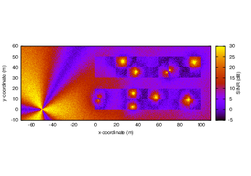
REM obtained from the lena-dual-stripe example
Note that the lena-dual-stripe example program also generate
gnuplot-compatible output files containing information about the
positions of the UE and eNB nodes as well as of the buildings,
respectively in the files ues.txt, enbs.txt and
buildings.txt. These can be easily included when using
gnuplot. For example, assuming that your gnuplot script (e.g., the
minimal gnuplot script described above) is saved in a file named
my_plot_script, running the following command would plot the
location of UEs, eNBs and buildings on top of the REM:
gnuplot -p enbs.txt ues.txt buildings.txt my_plot_script
AMC Model and CQI Calculation
The simulator provides two possible schemes for what concerns the selection of the MCSs and correspondingly the generation of the CQIs. The first one is based on the GSoC module [Piro2011] and works per RB basis. This model can be activated with the ns3 attribute system, as presented in the following:
Config::SetDefault ("ns3::LteAmc::AmcModel", EnumValue (LteAmc::PiroEW2010));
While, the solution based on the physical error model can be controlled with:
Config::SetDefault ("ns3::LteAmc::AmcModel", EnumValue (LteAmc::MiErrorModel));
Finally, the required efficiency of the PiroEW2010 AMC module can be tuned thanks to the Ber attribute (), for instance:
Config::SetDefault ("ns3::LteAmc::Ber", DoubleValue (0.00005));
Evolved Packet Core (EPC)
We now explain how to write a simulation program that allows to simulate the EPC in addition to the LTE radio access network. The use of EPC allows to use IPv4 and IPv6 networking with LTE devices. In other words, you will be able to use the regular ns-3 applications and sockets over IPv4 and IPv6 over LTE, and also to connect an LTE network to any other IPv4 and IPv6 network you might have in your simulation.
First of all, in addition to LteHelper that we already introduced
in Basic simulation program, you need to use an additional
EpcHelper class, which will take care of creating the EPC entities and
network topology. Note that you can’t use EpcHelper directly, as
it is an abstract base class; instead, you need to use one of its
child classes, which provide different EPC topology implementations. In
this example we will consider PointToPointEpcHelper, which
implements an EPC based on point-to-point links. To use it, you need
first to insert this code in your simulation program:
Ptr<LteHelper> lteHelper = CreateObject<LteHelper> ();
Ptr<PointToPointEpcHelper> epcHelper = CreateObject<PointToPointEpcHelper> ();
Then, you need to tell the LTE helper that the EPC will be used:
lteHelper->SetEpcHelper (epcHelper);
the above step is necessary so that the LTE helper will trigger the appropriate EPC configuration in correspondence with some important configuration, such as when a new eNB or UE is added to the simulation, or an EPS bearer is created. The EPC helper will automatically take care of the necessary setup, such as S1 link creation and S1 bearer setup. All this will be done without the intervention of the user.
Calling lteHelper->SetEpcHelper (epcHelper) enables the use of
EPC, and has the side effect that any new LteEnbRrc that is
created will have the EpsBearerToRlcMapping attribute set to
RLC_UM_ALWAYS instead of RLC_SM_ALWAYS if the latter was
the default; otherwise, the attribute won’t be changed (e.g., if
you changed the default to RLC_AM_ALWAYS, it won’t be touched).
It is to be noted that the EpcHelper will also automatically
create the PGW node and configure it so that it can properly handle
traffic from/to the LTE radio access network. Still,
you need to add some explicit code to connect the PGW to other
IPv4/IPv6 networks (e.g., the internet, another EPC). Here is a very
simple example about how to connect a single remote host (IPv4 type)
to the PGW via a point-to-point link:
Ptr<Node> pgw = epcHelper->GetPgwNode ();

// Create a single RemoteHost
NodeContainer remoteHostContainer;
remoteHostContainer.Create (1);
Ptr<Node> remoteHost = remoteHostContainer.Get (0);
InternetStackHelper internet;
internet.Install (remoteHostContainer);

// Create the internet
PointToPointHelper p2ph;
p2ph.SetDeviceAttribute ("DataRate", DataRateValue (DataRate ("100Gb/s")));
p2ph.SetDeviceAttribute ("Mtu", UintegerValue (1500));
p2ph.SetChannelAttribute ("Delay", TimeValue (Seconds (0.010)));
NetDeviceContainer internetDevices = p2ph.Install (pgw, remoteHost);
Ipv4AddressHelper ipv4h;
ipv4h.SetBase ("1.0.0.0", "255.0.0.0");
Ipv4InterfaceContainer internetIpIfaces = ipv4h.Assign (internetDevices);
// interface 0 is localhost, 1 is the p2p device
Ipv4Address remoteHostAddr = internetIpIfaces.GetAddress (1);


Ipv4StaticRoutingHelper ipv4RoutingHelper;
Ptr<Ipv4StaticRouting> remoteHostStaticRouting;
remoteHostStaticRouting = ipv4RoutingHelper.GetStaticRouting (remoteHost->GetObject<Ipv4> ());
remoteHostStaticRouting->AddNetworkRouteTo (epcHelper->GetEpcIpv4NetworkAddress (),
                                            Ipv4Mask ("255.255.0.0"), 1);
Now, you should go on and create LTE eNBs and UEs as explained in the previous sections. You can of course configure other LTE aspects such as pathloss and fading models. Right after you created the UEs, you should also configure them for IP networking. This is done as follows. We assume you have a container for UE and eNodeB nodes like this:
NodeContainer ueNodes;
NodeContainer enbNodes;
to configure an LTE-only simulation, you would then normally do something like this:
NetDeviceContainer ueLteDevs = lteHelper->InstallUeDevice (ueNodes);
lteHelper->Attach (ueLteDevs, enbLteDevs.Get (0));
in order to configure the UEs for IP networking, you just need to additionally do like this:
// we install the IP stack on the UEs
InternetStackHelper internet;
internet.Install (ueNodes);

// assign IP address to UEs
for (uint32_t u = 0; u < ueNodes.GetN (); ++u)
  {
    Ptr<Node> ue = ueNodes.Get (u);
    Ptr<NetDevice> ueLteDevice = ueLteDevs.Get (u);
    Ipv4InterfaceContainer ueIpIface;
    ueIpIface = epcHelper->AssignUeIpv4Address (NetDeviceContainer (ueLteDevice));
    // set the default gateway for the UE
    Ptr<Ipv4StaticRouting> ueStaticRouting;
    ueStaticRouting = ipv4RoutingHelper.GetStaticRouting (ue->GetObject<Ipv4> ());
    ueStaticRouting->SetDefaultRoute (epcHelper->GetUeDefaultGatewayAddress (), 1);
  }
The activation of bearers is done in a slightly different way with
respect to what done for an LTE-only simulation. First, the method
ActivateDataRadioBearer is not to be used when the EPC is
used. Second, when EPC is used, the default EPS bearer will be
activated automatically when you call LteHelper::Attach (). Third, if
you want to setup dedicated EPS bearer, you can do so using the method
LteHelper::ActivateDedicatedEpsBearer (). This method takes as a
parameter the Traffic Flow Template (TFT), which is a struct that
identifies the type of traffic that will be mapped to the dedicated
EPS bearer. Here is an example for how to setup a dedicated bearer
for an application at the UE communicating on port 1234:
Ptr<EpcTft> tft = Create<EpcTft> ();
EpcTft::PacketFilter pf;
pf.localPortStart = 1234;
pf.localPortEnd = 1234;
tft->Add (pf);
lteHelper->ActivateDedicatedEpsBearer (ueLteDevs,
                                       EpsBearer (EpsBearer::NGBR_VIDEO_TCP_DEFAULT),
                                       tft);
you can of course use custom EpsBearer and EpcTft configurations, please refer to the doxygen documentation for how to do it.
Finally, you can install applications on the LTE UE nodes that communicate with remote applications over the internet. This is done following the usual ns-3 procedures. Following our simple example with a single remoteHost, here is how to setup downlink communication, with an UdpClient application on the remote host, and a PacketSink on the LTE UE (using the same variable names of the previous code snippets)
uint16_t dlPort = 1234;
PacketSinkHelper packetSinkHelper ("ns3::UdpSocketFactory",
                                   InetSocketAddress (Ipv4Address::GetAny (), dlPort));
ApplicationContainer serverApps = packetSinkHelper.Install (ue);
serverApps.Start (Seconds (0.01));
UdpClientHelper client (ueIpIface.GetAddress (0), dlPort);
ApplicationContainer clientApps = client.Install (remoteHost);
clientApps.Start (Seconds (0.01));
That’s all! You can now start your simulation as usual:
Simulator::Stop (Seconds (10.0));
Simulator::Run ();
Using the EPC with emulation mode
In the previous section we used PointToPoint links for the connection between the eNBs and the SGW (S1-U interface) and among eNBs (X2-U and X2-C interfaces). The LTE module supports using emulated links instead of PointToPoint links. This is achieved by just replacing the creation of LteHelper and EpcHelper with the following code:
Ptr<LteHelper> lteHelper = CreateObject<LteHelper> ();
Ptr<EmuEpcHelper>  epcHelper = CreateObject<EmuEpcHelper> ();
lteHelper->SetEpcHelper (epcHelper);
epcHelper->Initialize ();
The attributes ns3::EmuEpcHelper::sgwDeviceName and ns3::EmuEpcHelper::enbDeviceName are used to set the name of the devices used for transporting the S1-U, X2-U and X2-C interfaces at the SGW and eNB, respectively. We will now show how this is done in an example where we execute the example program lena-simple-epc-emu using two virtual ethernet interfaces.
First of all we build ns-3 appropriately:
# configure
./waf configure --enable-sudo --enable-modules=lte,fd-net-device --enable-examples

# build
./waf
Then we setup two virtual ethernet interfaces, and start wireshark to look at the traffic going through:
# note: you need to be root

# create two paired veth devices
ip link add name veth0 type veth peer name veth1
ip link show

# enable promiscuous mode
ip link set veth0 promisc on
ip link set veth1 promisc on

# bring interfaces up
ip link set veth0 up
ip link set veth1 up

# start wireshark and capture on veth0
wireshark &
We can now run the example program with the simulated clock:
./waf --run lena-simple-epc-emu --command="%s --ns3::EmuEpcHelper::sgwDeviceName=veth0
--ns3::EmuEpcHelper::enbDeviceName=veth1"
Using wireshark, you should see ARP resolution first, then some GTP packets exchanged both in uplink and downlink.
The default setting of the example program is 1 eNB and 1UE. You can change this via command line parameters, e.g.:
./waf --run lena-simple-epc-emu --command="%s --ns3::EmuEpcHelper::sgwDeviceName=veth0
--ns3::EmuEpcHelper::enbDeviceName=veth1 --nEnbs=2 --nUesPerEnb=2"
To get a list of the available parameters:
./waf --run lena-simple-epc-emu --command="%s --PrintHelp"
To run with the realtime clock: it turns out that the default debug build is too slow for realtime. Softening the real time constraints with the BestEffort mode is not a good idea: something can go wrong (e.g., ARP can fail) and, if so, you won’t get any data packets out. So you need a decent hardware and the optimized build with statically linked modules:
./waf configure -d optimized --enable-static --enable-modules=lte --enable-examples
--enable-sudo
Then run the example program like this:
./waf --run lena-simple-epc-emu --command="%s --ns3::EmuEpcHelper::sgwDeviceName=veth0
--ns3::EmuEpcHelper::enbDeviceName=veth1
--SimulatorImplementationType=ns3::RealtimeSimulatorImpl
--ns3::RealtimeSimulatorImpl::SynchronizationMode=HardLimit"
note the HardLimit setting, which will cause the program to terminate if it cannot keep up with real time.
The approach described in this section can be used with any type of net device. For instance, [Baldo2014] describes how it was used to run an emulated LTE-EPC network over a real multi-layer packet-optical transport network.
Custom Backhaul
In the previous sections, Evolved Packet Core (EPC), we explained how to write a simulation
program using EPC with a predefined backhaul network between the RAN and the EPC. We used the
PointToPointEpcHelper. This EpcHelper creates point-to-point links between the eNBs and the SGW.
We now explain how to write a simulation program that allows the simulator user to create any kind of backhaul network in the simulation program.
First of all, in addition to LteHelper, you need to use the NoBackhaulEpcHelper class, which
implements an EPC but without connecting the eNBs with the core network. It just creates the network
elements of the core network:
Ptr<LteHelper> lteHelper = CreateObject<LteHelper> ();
Ptr<NoBackhaulEpcHelper> epcHelper = CreateObject<NoBackhaulEpcHelper> ();
Then, as usual, you need to tell the LTE helper that the EPC will be used:
lteHelper->SetEpcHelper (epcHelper);
Now, you should create the backhaul network. Here we create point-to-point links as it is done
by the PointToPointEpcHelper. We assume you have a container for eNB nodes like this:
NodeContainer enbNodes;
We get the SGW node:
Ptr<Node> sgw = epcHelper->GetSgwNode ();
And we connect every eNB from the container with the SGW with a point-to-point link. We also assign
IPv4 addresses to the interfaces of eNB and SGW with s1uIpv4AddressHelper.Assign (sgwEnbDevices)
and finally we tell the EpcHelper that this enb has a new S1 interface with
epcHelper->AddS1Interface (enb, enbS1uAddress, sgwS1uAddress), where enbS1uAddress and
sgwS1uAddress are the IPv4 addresses of the eNB and the SGW, respectively:
Ipv4AddressHelper s1uIpv4AddressHelper;

// Create networks of the S1 interfaces
s1uIpv4AddressHelper.SetBase ("10.0.0.0", "255.255.255.252");

for (uint16_t i = 0; i < enbNodes.GetN (); ++i)
  {
    Ptr<Node> enb = enbNodes.Get (i);

    // Create a point to point link between the eNB and the SGW with
    // the corresponding new NetDevices on each side
    PointToPointHelper p2ph;
    DataRate s1uLinkDataRate = DataRate ("10Gb/s");
    uint16_t s1uLinkMtu = 2000;
    Time s1uLinkDelay = Time (0);
    p2ph.SetDeviceAttribute ("DataRate", DataRateValue (s1uLinkDataRate));
    p2ph.SetDeviceAttribute ("Mtu", UintegerValue (s1uLinkMtu));
    p2ph.SetChannelAttribute ("Delay", TimeValue (s1uLinkDelay));
    NetDeviceContainer sgwEnbDevices = p2ph.Install (sgw, enb);

    Ipv4InterfaceContainer sgwEnbIpIfaces = s1uIpv4AddressHelper.Assign (sgwEnbDevices);
    s1uIpv4AddressHelper.NewNetwork ();

    Ipv4Address sgwS1uAddress = sgwEnbIpIfaces.GetAddress (0);
    Ipv4Address enbS1uAddress = sgwEnbIpIfaces.GetAddress (1);

    // Create S1 interface between the SGW and the eNB
    epcHelper->AddS1Interface (enb, enbS1uAddress, sgwS1uAddress);
  }
This is just an example how to create a custom backhaul network. In this other example, we connect all eNBs and the SGW to the same CSMA network:
// Create networks of the S1 interfaces
s1uIpv4AddressHelper.SetBase ("10.0.0.0", "255.255.255.0");

NodeContainer sgwEnbNodes;
sgwEnbNodes.Add (sgw);
sgwEnbNodes.Add (enbNodes);

CsmaHelper csmah;
NetDeviceContainer sgwEnbDevices = csmah.Install (sgwEnbNodes);
Ptr<NetDevice> sgwDev = sgwEnbDevices.Get (0);

Ipv4InterfaceContainer sgwEnbIpIfaces = s1uIpv4AddressHelper.Assign (sgwEnbDevices);
Ipv4Address sgwS1uAddress = sgwEnbIpIfaces.GetAddress (0);

for (uint16_t i = 0; i < enbNodes.GetN (); ++i)
  {
    Ptr<Node> enb = enbNodes.Get (i);
    Ipv4Address enbS1uAddress = sgwEnbIpIfaces.GetAddress (i + 1);

    // Create S1 interface between the SGW and the eNB
    epcHelper->AddS1Interface (enb, enbS1uAddress, sgwS1uAddress);
  }
As you can see, apart from how you create the backhaul network, i.e. the point-to-point links or
the CSMA network, the important point is to tell the EpcHelper that an eNB has a new S1 interface.
Now, you should continue configuring your simulation program as it is explained in Evolved Packet Core (EPC) subsection. This configuration includes: the internet, installing the LTE eNBs and possibly configuring other LTE aspects, installing the LTE UEs and configuring them as IP nodes, activation of the dedicated EPS bearers and installing applications on the LTE UEs and on the remote hosts.
Network Attachment
As shown in the basic example in section Basic simulation program,
attaching a UE to an eNodeB is done by calling LteHelper::Attach function.
There are 2 possible ways of network attachment. The first method is the “manual” one, while the second one has a more “automatic” sense on it. Each of them will be covered in this section.
Manual attachment
This method uses the LteHelper::Attach function mentioned above. It has been
the only available network attachment method in earlier versions of LTE module.
It is typically invoked before the simulation begins:
lteHelper->Attach (ueDevs, enbDev); // attach one or more UEs to a single eNodeB
LteHelper::InstallEnbDevice and LteHelper::InstallUeDevice functions
must have been called before attaching. In an EPC-enabled simulation, it is also
required to have IPv4/IPv6 properly pre-installed in the UE.
This method is very simple, but requires you to know exactly which UE belongs to to which eNodeB before the simulation begins. This can be difficult when the UE initial position is randomly determined by the simulation script.
One may choose the distance between the UE and the eNodeB as a criterion for selecting the appropriate cell. It is quite simple (at least from the simulator’s point of view) and sometimes practical. But it is important to note that sometimes distance does not make a single correct criterion. For instance, the eNodeB antenna directivity should be considered as well. Besides that, one should also take into account the channel condition, which might be fluctuating if there is fading or shadowing in effect. In these kind of cases, network attachment should not be based on distance alone.
In real life, UE will automatically evaluate certain criteria and select the
best cell to attach to, without manual intervention from the user. Obviously
this is not the case in this LteHelper::Attach function. The other network
attachment method uses more “automatic” approach to network attachment, as
will be described next.
Automatic attachment using Idle mode cell selection procedure
The strength of the received signal is the standard criterion used for selecting
the best cell to attach to. The use of this criterion is implemented in the
initial cell selection process, which can be invoked by calling another
version of the LteHelper::Attach function, as shown below:
lteHelper->Attach (ueDevs); // attach one or more UEs to a strongest cell
The difference with the manual method is that the destination eNodeB is not specified. The procedure will find the best cell for the UEs, based on several criteria, including the strength of the received signal (RSRP).
After the method is called, the UE will spend some time to measure the neighbouring cells, and then attempt to attach to the best one. More details can be found in section Initial Cell Selection of the Design Documentation.
It is important to note that this method only works in EPC-enabled simulations. LTE-only simulations must resort to manual attachment method.
Closed Subscriber Group
An interesting use case of the initial cell selection process is to setup a simulation environment with Closed Subscriber Group (CSG).
For example, a certain eNodeB, typically a smaller version such as femtocell, might belong to a private owner (e.g. a household or business), allowing access only to some UEs which have been previously registered by the owner. The eNodeB and the registered UEs altogether form a CSG.
The access restriction can be simulated by “labeling” the CSG members with the
same CSG ID. This is done through the attributes in both eNodeB and UE, for
example using the following LteHelper functions:
// label the following eNodeBs with CSG identity of 1 and CSG indication enabled
lteHelper->SetEnbDeviceAttribute ("CsgId", UintegerValue (1));
lteHelper->SetEnbDeviceAttribute ("CsgIndication", BooleanValue (true));

// label one or more UEs with CSG identity of 1
lteHelper->SetUeDeviceAttribute ("CsgId", UintegerValue (1));

// install the eNodeBs and UEs
NetDeviceContainer csgEnbDevs = lteHelper->InstallEnbDevice (csgEnbNodes);
NetDeviceContainer csgUeDevs = lteHelper->InstallUeDevice (csgUeNodes);
Then enable the initial cell selection procedure on the UEs:
lteHelper->Attach (csgUeDevs);
This is necessary because the CSG restriction only works with automatic method of network attachment, but not in the manual method.
Note that setting the CSG indication of an eNodeB as false (the default value) will disable the restriction, i.e., any UEs can connect to this eNodeB.
Configure UE measurements
The active UE measurement configuration in a simulation is dictated by the selected so called “consumers”, such as handover algorithm. Users may add their own configuration into action, and there are several ways to do so:
- direct configuration in eNodeB RRC entity;
- configuring existing handover algorithm; and
- developing a new handover algorithm.
This section will cover the first method only. The second method is covered in Automatic handover trigger, while the third method is explained in length in Section Handover algorithm of the Design Documentation.
Direct configuration in eNodeB RRC works as follows. User begins by creating a
new LteRrcSap::ReportConfigEutra instance and pass it to the
LteEnbRrc::AddUeMeasReportConfig function. The function will return the
measId (measurement identity) which is a unique reference of the
configuration in the eNodeB instance. This function must be called before the
simulation begins. The measurement configuration will be active in all UEs
attached to the eNodeB throughout the duration of the simulation. During the
simulation, user can capture the measurement reports produced by the UEs by
listening to the existing LteEnbRrc::RecvMeasurementReport trace source.
The structure ReportConfigEutra is in accord with 3GPP specification. Definition of the structure and each member field can be found in Section 6.3.5 of [TS36331].
The code sample below configures Event A1 RSRP measurement to every eNodeB
within the container devs:
LteRrcSap::ReportConfigEutra config;
config.eventId = LteRrcSap::ReportConfigEutra::EVENT_A1;
config.threshold1.choice = LteRrcSap::ThresholdEutra::THRESHOLD_RSRP;
config.threshold1.range = 41;
config.triggerQuantity = LteRrcSap::ReportConfigEutra::RSRP;
config.reportInterval = LteRrcSap::ReportConfigEutra::MS480;

std::vector<uint8_t> measIdList;

NetDeviceContainer::Iterator it;
for (it = devs.Begin (); it != devs.End (); it++)
{
  Ptr<NetDevice> dev = *it;
  Ptr<LteEnbNetDevice> enbDev = dev->GetObject<LteEnbNetDevice> ();
  Ptr<LteEnbRrc> enbRrc = enbDev->GetRrc ();

  uint8_t measId = enbRrc->AddUeMeasReportConfig (config);
  measIdList.push_back (measId); // remember the measId created

  enbRrc->TraceConnect ("RecvMeasurementReport",
                        "context",
                        MakeCallback (&RecvMeasurementReportCallback));
}
Note that thresholds are expressed as range. In the example above, the range 41
for RSRP corresponds to -100 dBm. The conversion from and to the range format is
due to Section 9.1.4 and 9.1.7 of [TS36133]. The EutranMeasurementMapping
class has several static functions that can be used for this purpose.
The corresponding callback function would have a definition similar as below:
void
RecvMeasurementReportCallback (std::string context,
                               uint64_t imsi,
                               uint16_t cellId,
                               uint16_t rnti,
                               LteRrcSap::MeasurementReport measReport);
This method will register the callback function as a consumer of UE
measurements. In the case where there are more than one consumers in the
simulation (e.g. handover algorithm), the measurements intended for other
consumers will also be captured by this callback function. Users may utilize the
the measId field, contained within the LteRrcSap::MeasurementReport
argument of the callback function, to tell which measurement configuration has
triggered the report.
In general, this mechanism prevents one consumer to unknowingly intervene with another consumer’s reporting configuration.
Note that only the reporting configuration part (i.e.
LteRrcSap::ReportConfigEutra) of the UE measurements parameter is open for
consumers to configure, while the other parts are kept hidden. The
intra-frequency limitation is the main motivation behind this API implementation
decision:
- there is only one, unambiguous and definitive measurement object, thus there is no need to configure it;
- measurement identities are kept hidden because of the fact that there is one-to-one mapping between reporting configuration and measurement identity, thus a new measurement identity is set up automatically when a new reporting configuration is created;
- quantity configuration is configured elsewhere, see Performing measurements; and
- measurement gaps are not supported, because it is only applicable for inter-frequency settings;
X2-based handover
As defined by 3GPP, handover is a procedure for changing the serving cell of a UE in CONNECTED mode. The two eNodeBs involved in the process are typically called the source eNodeB and the target eNodeB.
In order to enable the execution of X2-based handover in simulation, there are two requirements that must be met. Firstly, EPC must be enabled in the simulation (see Evolved Packet Core (EPC)).
Secondly, an X2 interface must be configured between the two eNodeBs, which needs to be done explicitly within the simulation program:
lteHelper->AddX2Interface (enbNodes);
where enbNodes is a NodeContainer that contains the two eNodeBs between
which the X2 interface is to be configured. If the container has more than two
eNodeBs, the function will create an X2 interface between every pair of eNodeBs
in the container.
Lastly, the target eNodeB must be configured as “open” to X2 HANDOVER REQUEST.
Every eNodeB is open by default, so no extra instruction is needed in most
cases. However, users may set the eNodeB to “closed” by setting the boolean
attribute LteEnbRrc::AdmitHandoverRequest to false. As an example, you can
run the lena-x2-handover program and setting the attribute in this way:
NS_LOG=EpcX2:LteEnbRrc ./waf --run lena-x2-handover --command="%s --ns3::LteEnbRrc::AdmitHandoverRequest=false"
After the above three requirements are fulfilled, the handover procedure can be triggered manually or automatically. Each will be presented in the following subsections.
Manual handover trigger
Handover event can be triggered “manually” within the simulation program by
scheduling an explicit handover event. The LteHelper object provides a
convenient method for the scheduling of a handover event. As an example, let us
assume that ueLteDevs is a NetDeviceContainer that contains the UE that
is to be handed over, and that enbLteDevs is another NetDeviceContainer
that contains the source and the target eNB. Then, a handover at 0.1s can be
scheduled like this:
lteHelper->HandoverRequest (Seconds (0.100),
                            ueLteDevs.Get (0),
                            enbLteDevs.Get (0),
                            enbLteDevs.Get (1));
Note that the UE needs to be already connected to the source eNB, otherwise the simulation will terminate with an error message.
For an example with full source code, please refer to the lena-x2-handover
example program.
Automatic handover trigger
Handover procedure can also be triggered “automatically” by the serving eNodeB of the UE. The logic behind the trigger depends on the handover algorithm currently active in the eNodeB RRC entity. Users may select and configure the handover algorithm that will be used in the simulation, which will be explained shortly in this section. Users may also opt to write their own implementation of handover algorithm, as described in Section Handover algorithm of the Design Documentation.
Selecting a handover algorithm is done via the LteHelper object and its
SetHandoverAlgorithmType method as shown below:
Ptr<LteHelper> lteHelper = CreateObject<LteHelper> ();
lteHelper->SetHandoverAlgorithmType ("ns3::A2A4RsrqHandoverAlgorithm");
The selected handover algorithm may also provide several configurable attributes, which can be set as follows:
lteHelper->SetHandoverAlgorithmAttribute ("ServingCellThreshold",
                                          UintegerValue (30));
lteHelper->SetHandoverAlgorithmAttribute ("NeighbourCellOffset",
                                          UintegerValue (1));
Three options of handover algorithm are included in the LTE module. The
A2-A4-RSRQ handover algorithm (named as ns3::A2A4RsrqHandoverAlgorithm) is
the default option, and the usage has already been shown above.
Another option is the strongest cell handover algorithm (named as
ns3::A3RsrpHandoverAlgorithm), which can be selected and configured by the
following code:
lteHelper->SetHandoverAlgorithmType ("ns3::A3RsrpHandoverAlgorithm");
lteHelper->SetHandoverAlgorithmAttribute ("Hysteresis",
                                          DoubleValue (3.0));
lteHelper->SetHandoverAlgorithmAttribute ("TimeToTrigger",
                                          TimeValue (MilliSeconds (256)));
The last option is a special one, called the no-op handover algorithm, which basically disables automatic handover trigger. This is useful for example in cases where manual handover trigger need an exclusive control of all handover decision. It does not have any configurable attributes. The usage is as follows:
lteHelper->SetHandoverAlgorithmType ("ns3::NoOpHandoverAlgorithm");
For more information on each handover algorithm’s decision policy and their attributes, please refer to their respective subsections in Section Handover algorithm of the Design Documentation.
Finally, the InstallEnbDevice function of LteHelper will instantiate one
instance of the selected handover algorithm for each eNodeB device. In other
words, make sure to select the right handover algorithm before finalizing it in
the following line of code:
NetDeviceContainer enbLteDevs = lteHelper->InstallEnbDevice (enbNodes);
Example with full source code of using automatic handover trigger can be found
in the lena-x2-handover-measures example program.
Tuning simulation with handover
As mentioned in the Design Documentation, the current implementation of handover model may produce unpredicted behaviour when handover failure occurs. This subsection will focus on the steps that should be taken into account by users if they plan to use handover in their simulations.
The major cause of handover failure that we will tackle is the error in transmitting handover-related signaling messages during the execution of a handover procedure. As apparent from the Figure Sequence diagram of the X2-based handover from the Design Documentation, there are many of them and they use different interfaces and protocols. For the sake of simplicity, we can safely assume that the X2 interface (between the source eNodeB and the target eNodeB) and the S1 interface (between the target eNodeB and the SGW/PGW) are quite stable. Therefore we will focus our attention to the RRC protocol (between the UE and the eNodeBs) and the Random Access procedure, which are normally transmitted through the air and susceptible to degradation of channel condition.
A general tips to reduce transmission error is to ensure high enough SINR level in every UE. This can be done by a proper planning of the network topology that minimizes network coverage hole. If the topology has a known coverage hole, then the UE should be configured not to venture to that area.
Another approach to keep in mind is to avoid too-late handovers. In other words, handover should happen before the UE’s SINR becomes too low, otherwise the UE may fail to receive the handover command from the source eNodeB. Handover algorithms have the means to control how early or late a handover decision is made. For example, A2-A4-RSRQ handover algorithm can be configured with a higher threshold to make it decide a handover earlier. Similarly, smaller hysteresis and/or shorter time-to-trigger in the strongest cell handover algorithm typically results in earlier handovers. In order to find the right values for these parameters, one of the factors that should be considered is the UE movement speed. Generally, a faster moving UE requires the handover to be executed earlier. Some research work have suggested recommended values, such as in [Lee2010].
The above tips should be enough in normal simulation uses, but in the case some special needs arise then an extreme measure can be taken into consideration. For instance, users may consider disabling the channel error models. This will ensure that all handover-related signaling messages will be transmitted successfully, regardless of distance and channel condition. However, it will also affect all other data or control packets not related to handover, which may be an unwanted side effect. Otherwise, it can be done as follows:
Config::SetDefault ("ns3::LteSpectrumPhy::CtrlErrorModelEnabled", BooleanValue (false));
Config::SetDefault ("ns3::LteSpectrumPhy::DataErrorModelEnabled", BooleanValue (false));
By using the above code, we disable the error model in both control and data channels and in both directions (downlink and uplink). This is necessary because handover-related signaling messages are transmitted using these channels. An exception is when the simulation uses the ideal RRC protocol. In this case, only the Random Access procedure is left to be considered. The procedure consists of control messages, therefore we only need to disable the control channel’s error model.
Handover traces
The RRC model, in particular the LteEnbRrc and LteUeRrc
objects, provide some useful traces which can be hooked up to some
custom functions so that they are called upon start and end of the
handover execution phase at both the UE and eNB side. As an example,
in your simulation program you can declare the following methods:
void
NotifyHandoverStartUe (std::string context,
                       uint64_t imsi,
                       uint16_t cellId,
                       uint16_t rnti,
                       uint16_t targetCellId)
{
  std::cout << Simulator::Now ().GetSeconds () << " " << context
            << " UE IMSI " << imsi
            << ": previously connected to CellId " << cellId
            << " with RNTI " << rnti
            << ", doing handover to CellId " << targetCellId
            << std::endl;
}

void
NotifyHandoverEndOkUe (std::string context,
                       uint64_t imsi,
                       uint16_t cellId,
                       uint16_t rnti)
{
  std::cout << Simulator::Now ().GetSeconds () << " " << context
            << " UE IMSI " << imsi
            << ": successful handover to CellId " << cellId
            << " with RNTI " << rnti
            << std::endl;
}

void
NotifyHandoverStartEnb (std::string context,
                        uint64_t imsi,
                        uint16_t cellId,
                        uint16_t rnti,
                        uint16_t targetCellId)
{
  std::cout << Simulator::Now ().GetSeconds () << " " << context
            << " eNB CellId " << cellId
            << ": start handover of UE with IMSI " << imsi
            << " RNTI " << rnti
            << " to CellId " << targetCellId
            << std::endl;
}

void
NotifyHandoverEndOkEnb (std::string context,
                        uint64_t imsi,
                        uint16_t cellId,
                        uint16_t rnti)
{
  std::cout << Simulator::Now ().GetSeconds () << " " << context
            << " eNB CellId " << cellId
            << ": completed handover of UE with IMSI " << imsi
            << " RNTI " << rnti
            << std::endl;
}
Then, you can hook up these methods to the corresponding trace sources like this:
Config::Connect ("/NodeList/*/DeviceList/*/LteEnbRrc/HandoverStart",
                 MakeCallback (&NotifyHandoverStartEnb));
Config::Connect ("/NodeList/*/DeviceList/*/LteUeRrc/HandoverStart",
                 MakeCallback (&NotifyHandoverStartUe));
Config::Connect ("/NodeList/*/DeviceList/*/LteEnbRrc/HandoverEndOk",
                 MakeCallback (&NotifyHandoverEndOkEnb));
Config::Connect ("/NodeList/*/DeviceList/*/LteUeRrc/HandoverEndOk",
                 MakeCallback (&NotifyHandoverEndOkUe));
The example program src/lte/examples/lena-x2-handover.cc
illustrates how the all above instructions can be integrated in a
simulation program. You can run the program like this:
./waf --run lena-x2-handover
and it will output the messages printed by the custom handover trace hooks. In order additionally visualize some meaningful logging information, you can run the program like this:
NS_LOG=LteEnbRrc:LteUeRrc:EpcX2 ./waf --run lena-x2-handover
Frequency Reuse Algorithms
In this section we will describe how to use Frequency Reuse Algorithms in eNb within LTE simulations. There are two possible ways of configuration. The first approach is the “manual” one, it requires more parameters to be configured, but allow user to configure FR algorithm as he/she needs. The second approach is more “automatic”. It is very convenient, because is the same for each FR algorithm, so user can switch FR algorithm very quickly by changing only type of FR algorithm. One drawback is that “automatic” approach uses only limited set of configurations for each algorithm, what make it less flexible, but is sufficient for most of cases.
These two approaches will be described more in following sub-section.
If user do not configure Frequency Reuse algorithm, default one (i.e. LteFrNoOpAlgorithm) is installed in eNb. It acts as if FR algorithm was disabled.
One thing that should be mentioned is that most of implemented FR algorithms work with cell bandwidth greater or equal than 15 RBs. This limitation is caused by requirement that at least three continuous RBs have to be assigned to UE for transmission.
Manual configuration
Frequency reuse algorithm can be configured “manually” within the simulation program by setting type of FR algorithm and all its attributes. Currently, seven FR algorithms are implemented:
ns3::LteFrNoOpAlgorithmns3::LteFrHardAlgorithmns3::LteFrStrictAlgorithmns3::LteFrSoftAlgorithmns3::LteFfrSoftAlgorithmns3::LteFfrEnhancedAlgorithmns3::LteFfrDistributedAlgorithm
Selecting a FR algorithm is done via the LteHelper object and
its SetFfrAlgorithmType method as shown below:
Ptr<LteHelper> lteHelper = CreateObject<LteHelper> ();
lteHelper->SetFfrAlgorithmType ("ns3::LteFrHardAlgorithm");
Each implemented FR algorithm provide several configurable attributes. Users do
not have to care about UL and DL bandwidth configuration, because it is done
automatically during cell configuration. To change bandwidth for FR algorithm,
configure required values for LteEnbNetDevice:
uint8_t bandwidth = 100;
lteHelper->SetEnbDeviceAttribute ("DlBandwidth", UintegerValue (bandwidth));
lteHelper->SetEnbDeviceAttribute ("UlBandwidth", UintegerValue (bandwidth));
Now, each FR algorithms configuration will be described.
Hard Frequency Reuse Algorithm
As described in Section Hard Frequency Reuse of the Design Documentation
ns3::LteFrHardAlgorithm uses one sub-band. To configure this sub-band user need
to specify offset and bandwidth for DL and UL in number of RBs.
Hard Frequency Reuse Algorithm provides following attributes:
DlSubBandOffset: Downlink Offset in number of Resource Block GroupsDlSubBandwidth: Downlink Transmission SubBandwidth Configuration in number of Resource Block GroupsUlSubBandOffset: Uplink Offset in number of Resource Block GroupsUlSubBandwidth: Uplink Transmission SubBandwidth Configuration in number of Resource Block Groups
Example configuration of LteFrHardAlgorithm can be done in following way:
lteHelper->SetFfrAlgorithmType ("ns3::LteFrHardAlgorithm");
lteHelper->SetFfrAlgorithmAttribute ("DlSubBandOffset", UintegerValue (8));
lteHelper->SetFfrAlgorithmAttribute ("DlSubBandwidth", UintegerValue (8));
lteHelper->SetFfrAlgorithmAttribute ("UlSubBandOffset", UintegerValue (8));
lteHelper->SetFfrAlgorithmAttribute ("UlSubBandwidth", UintegerValue (8));
NetDeviceContainer enbDevs = lteHelper->InstallEnbDevice (enbNodes.Get(0));
Above example allow eNB to use only RBs from 8 to 16 in DL and UL, while entire cell bandwidth is 25.
Strict Frequency Reuse Algorithm
Strict Frequency Reuse Algorithm uses two sub-bands: one common for each cell and one private. There is also RSRQ threshold, which is needed to decide within which sub-band UE should be served. Moreover the power transmission in these sub-bands can be different.
Strict Frequency Reuse Algorithm provides following attributes:
UlCommonSubBandwidth: Uplink Common SubBandwidth Configuration in number of Resource Block GroupsUlEdgeSubBandOffset: Uplink Edge SubBand Offset in number of Resource Block GroupsUlEdgeSubBandwidth: Uplink Edge SubBandwidth Configuration in number of Resource Block GroupsDlCommonSubBandwidth: Downlink Common SubBandwidth Configuration in number of Resource Block GroupsDlEdgeSubBandOffset: Downlink Edge SubBand Offset in number of Resource Block GroupsDlEdgeSubBandwidth: Downlink Edge SubBandwidth Configuration in number of Resource Block GroupsRsrqThreshold: If the RSRQ of is worse than this threshold, UE should be served in edge sub-bandCenterPowerOffset: PdschConfigDedicated::Pa value for center sub-band, default value dB0EdgePowerOffset: PdschConfigDedicated::Pa value for edge sub-band, default value dB0CenterAreaTpc: TPC value which will be set in DL-DCI for UEs in center area, Absolute mode is used, default value 1 is mapped to -1 according to TS36.213 Table 5.1.1.1-2EdgeAreaTpc: TPC value which will be set in DL-DCI for UEs in edge area, Absolute mode is used, default value 1 is mapped to -1 according to TS36.213 Table 5.1.1.1-2
Example below allow eNB to use RBs from 0 to 6 as common sub-band and from 12 to 18 as
private sub-band in DL and UL, RSRQ threshold is 20 dB, power in center area equals
LteEnbPhy::TxPower - 3dB, power in edge area equals LteEnbPhy::TxPower + 3dB:
lteHelper->SetFfrAlgorithmType ("ns3::LteFrStrictAlgorithm");
lteHelper->SetFfrAlgorithmAttribute ("DlCommonSubBandwidth", UintegerValue (6));
lteHelper->SetFfrAlgorithmAttribute ("UlCommonSubBandwidth", UintegerValue (6));
lteHelper->SetFfrAlgorithmAttribute ("DlEdgeSubBandOffset", UintegerValue (6));
lteHelper->SetFfrAlgorithmAttribute ("DlEdgeSubBandwidth", UintegerValue (6));
lteHelper->SetFfrAlgorithmAttribute ("UlEdgeSubBandOffset", UintegerValue (6));
lteHelper->SetFfrAlgorithmAttribute ("UlEdgeSubBandwidth", UintegerValue (6));
lteHelper->SetFfrAlgorithmAttribute ("RsrqThreshold", UintegerValue (20));
lteHelper->SetFfrAlgorithmAttribute ("CenterPowerOffset",
                      UintegerValue (LteRrcSap::PdschConfigDedicated::dB_3));
lteHelper->SetFfrAlgorithmAttribute ("EdgePowerOffset",
                      UintegerValue (LteRrcSap::PdschConfigDedicated::dB3));
lteHelper->SetFfrAlgorithmAttribute ("CenterAreaTpc", UintegerValue (1));
lteHelper->SetFfrAlgorithmAttribute ("EdgeAreaTpc", UintegerValue (2));
NetDeviceContainer enbDevs = lteHelper->InstallEnbDevice (enbNodes.Get(0));
Soft Frequency Reuse Algorithm
With Soft Frequency Reuse Algorithm, eNb uses entire cell bandwidth, but there are two sub-bands, within UEs are served with different power level.
Soft Frequency Reuse Algorithm provides following attributes:
UlEdgeSubBandOffset: Uplink Edge SubBand Offset in number of Resource Block GroupsUlEdgeSubBandwidth: Uplink Edge SubBandwidth Configuration in number of Resource Block GroupsDlEdgeSubBandOffset: Downlink Edge SubBand Offset in number of Resource Block GroupsDlEdgeSubBandwidth: Downlink Edge SubBandwidth Configuration in number of Resource Block GroupsAllowCenterUeUseEdgeSubBand: If true center UEs can receive on edge sub-band RBGs, otherwise edge sub-band is allowed only for edge UEs, default value is trueRsrqThreshold: If the RSRQ of is worse than this threshold, UE should be served in edge sub-bandCenterPowerOffset: PdschConfigDedicated::Pa value for center sub-band, default value dB0EdgePowerOffset: PdschConfigDedicated::Pa value for edge sub-band, default value dB0CenterAreaTpc: TPC value which will be set in DL-DCI for UEs in center area, Absolute mode is used, default value 1 is mapped to -1 according to TS36.213 Table 5.1.1.1-2EdgeAreaTpc: TPC value which will be set in DL-DCI for UEs in edge area, Absolute mode is used, default value 1 is mapped to -1 according to TS36.213 Table 5.1.1.1-2
Example below configures RBs from 8 to 16 to be used by cell edge UEs and this sub-band
is not available for cell center users. RSRQ threshold is 20 dB, power in center area
equals LteEnbPhy::TxPower, power in edge area equals LteEnbPhy::TxPower + 3dB:
lteHelper->SetFfrAlgorithmType ("ns3::LteFrSoftAlgorithm");
lteHelper->SetFfrAlgorithmAttribute ("DlEdgeSubBandOffset", UintegerValue (8));
lteHelper->SetFfrAlgorithmAttribute ("DlEdgeSubBandwidth", UintegerValue (8));
lteHelper->SetFfrAlgorithmAttribute ("UlEdgeSubBandOffset", UintegerValue (8));
lteHelper->SetFfrAlgorithmAttribute ("UlEdgeSubBandwidth", UintegerValue (8));
lteHelper->SetFfrAlgorithmAttribute ("AllowCenterUeUseEdgeSubBand", BooleanValue (false));
lteHelper->SetFfrAlgorithmAttribute ("RsrqThreshold", UintegerValue (20));
lteHelper->SetFfrAlgorithmAttribute ("CenterPowerOffset",
                      UintegerValue (LteRrcSap::PdschConfigDedicated::dB0));
lteHelper->SetFfrAlgorithmAttribute ("EdgePowerOffset",
                      UintegerValue (LteRrcSap::PdschConfigDedicated::dB3));
NetDeviceContainer enbDevs = lteHelper->InstallEnbDevice (enbNodes.Get(0));
Soft Fractional Frequency Reuse Algorithm
Soft Fractional Frequency Reuse (SFFR) uses three sub-bands: center, medium (common) and edge. User have to configure only two of them: common and edge. Center sub-band will be composed from the remaining bandwidth. Each sub-band can be served with different transmission power. Since there are three sub-bands, two RSRQ thresholds needs to be configured.
Soft Fractional Frequency Reuse Algorithm provides following attributes:
UlCommonSubBandwidth: Uplink Common SubBandwidth Configuration in number of Resource Block GroupsUlEdgeSubBandOffset: Uplink Edge SubBand Offset in number of Resource Block GroupsUlEdgeSubBandwidth: Uplink Edge SubBandwidth Configuration in number of Resource Block GroupsDlCommonSubBandwidth: Downlink Common SubBandwidth Configuration in number of Resource Block GroupsDlEdgeSubBandOffset: Downlink Edge SubBand Offset in number of Resource Block GroupsDlEdgeSubBandwidth: Downlink Edge SubBandwidth Configuration in number of Resource Block GroupsCenterRsrqThreshold: If the RSRQ of is worse than this threshold, UE should be served in medium sub-bandEdgeRsrqThreshold: If the RSRQ of is worse than this threshold, UE should be served in edge sub-bandCenterAreaPowerOffset: PdschConfigDedicated::Pa value for center sub-band, default value dB0MediumAreaPowerOffset: PdschConfigDedicated::Pa value for medium sub-band, default value dB0EdgeAreaPowerOffset: PdschConfigDedicated::Pa value for edge sub-band, default value dB0CenterAreaTpc: TPC value which will be set in DL-DCI for UEs in center area, Absolute mode is used, default value 1 is mapped to -1 according to TS36.213 Table 5.1.1.1-2MediumAreaTpc: TPC value which will be set in DL-DCI for UEs in medium area, Absolute mode is used, default value 1 is mapped to -1 according to TS36.213 Table 5.1.1.1-2EdgeAreaTpc: TPC value which will be set in DL-DCI for UEs in edge area, Absolute mode is used, default value 1 is mapped to -1 according to TS36.213 Table 5.1.1.1-2
In example below RBs from 0 to 6 will be used as common (medium) sub-band,
RBs from 6 to 12 will be used as edge sub-band and RBs from 12 to 24 will be used as
center sub-band (it is composed with remaining RBs). RSRQ threshold between center
and medium area is 28 dB, RSRQ threshold between medium and edge area is 18 dB.
Power in center area equals LteEnbPhy::TxPower - 3dB, power in medium area equals
LteEnbPhy::TxPower + 3dB, power in edge area equals LteEnbPhy::TxPower + 3dB:
lteHelper->SetFfrAlgorithmType ("ns3::LteFfrSoftAlgorithm");
lteHelper->SetFfrAlgorithmAttribute ("UlCommonSubBandwidth", UintegerValue (6));
lteHelper->SetFfrAlgorithmAttribute ("DlCommonSubBandwidth", UintegerValue (6));
lteHelper->SetFfrAlgorithmAttribute ("DlEdgeSubBandOffset", UintegerValue (0));
lteHelper->SetFfrAlgorithmAttribute ("DlEdgeSubBandwidth", UintegerValue (6));
lteHelper->SetFfrAlgorithmAttribute ("UlEdgeSubBandOffset", UintegerValue (0));
lteHelper->SetFfrAlgorithmAttribute ("UlEdgeSubBandwidth", UintegerValue (6));
lteHelper->SetFfrAlgorithmAttribute ("CenterRsrqThreshold", UintegerValue (28));
lteHelper->SetFfrAlgorithmAttribute ("EdgeRsrqThreshold", UintegerValue (18));
lteHelper->SetFfrAlgorithmAttribute ("CenterAreaPowerOffset",
                      UintegerValue (LteRrcSap::PdschConfigDedicated::dB_3));
lteHelper->SetFfrAlgorithmAttribute ("MediumAreaPowerOffset",
                      UintegerValue (LteRrcSap::PdschConfigDedicated::dB0));
lteHelper->SetFfrAlgorithmAttribute ("EdgeAreaPowerOffset",
                      UintegerValue (LteRrcSap::PdschConfigDedicated::dB3));
NetDeviceContainer enbDevs = lteHelper->InstallEnbDevice (enbNodes.Get(0));
Enhanced Fractional Frequency Reuse Algorithm
Enhanced Fractional Frequency Reuse (EFFR) reserve part of system bandwidth for each cell
(typically there are 3 cell types and each one gets 1/3 of system bandwidth). Then part of
this subbandwidth it used as Primary Segment with reuse factor 3 and as Secondary Segment
with reuse factor 1. User has to configure (for DL and UL) offset of the cell subbandwidth
in number of RB, number of RB which will be used as Primary Segment and number of RB which
will be used as Secondary Segment. Primary Segment is used by cell at will, but RBs from
Secondary Segment can be assigned to UE only is CQI feedback from this UE have higher value
than configured CQI threshold. UE is considered as edge UE when its RSRQ is lower than RsrqThreshold.
Since each eNb needs to know where are Primary and Secondary of other cell types, it will calculate them assuming configuration is the same for each cell and only subbandwidth offsets are different. So it is important to divide available system bandwidth equally to each cell and apply the same configuration of Primary and Secondary Segments to them.
Enhanced Fractional Frequency Reuse Algorithm provides following attributes:
UlSubBandOffset: Uplink SubBand Offset for this cell in number of Resource Block GroupsUlReuse3SubBandwidth: Uplink Reuse 3 SubBandwidth Configuration in number of Resource Block GroupsUlReuse1SubBandwidth: Uplink Reuse 1 SubBandwidth Configuration in number of Resource Block GroupsDlSubBandOffset: Downlink SubBand Offset for this cell in number of Resource Block GroupsDlReuse3SubBandwidth: Downlink Reuse 3 SubBandwidth Configuration in number of Resource Block GroupsDlReuse1SubBandwidth: Downlink Reuse 1 SubBandwidth Configuration in number of Resource Block GroupsRsrqThreshold: If the RSRQ of is worse than this threshold, UE should be served in edge sub-bandCenterAreaPowerOffset: PdschConfigDedicated::Pa value for center sub-band, default value dB0EdgeAreaPowerOffset: PdschConfigDedicated::Pa value for edge sub-band, default value dB0DlCqiThreshold: If the DL-CQI for RBG of is higher than this threshold, transmission on RBG is possibleUlCqiThreshold: If the UL-CQI for RBG of is higher than this threshold, transmission on RBG is possibleCenterAreaTpc: TPC value which will be set in DL-DCI for UEs in center area, Absolute mode is used, default value 1 is mapped to -1 according to TS36.213 Table 5.1.1.1-2EdgeAreaTpc: TPC value which will be set in DL-DCI for UEs in edge area, Absolute mode is used, default value 1 is mapped to -1 according to TS36.213 Table 5.1.1.1-2
In example below offset in DL and UL is 0 RB, 4 RB will be used in Primary Segment and
Secondary Segment. RSRQ threshold between center and edge area is 25 dB. DL and UL CQI
thresholds are set to value of 10. Power in center area equals LteEnbPhy::TxPower - 6dB,
power in edge area equals LteEnbPhy::TxPower + 0dB:
lteHelper->SetFfrAlgorithmType("ns3::LteFfrEnhancedAlgorithm");
lteHelper->SetFfrAlgorithmAttribute("RsrqThreshold", UintegerValue (25));
lteHelper->SetFfrAlgorithmAttribute("DlCqiThreshold", UintegerValue (10));
lteHelper->SetFfrAlgorithmAttribute("UlCqiThreshold", UintegerValue (10));
lteHelper->SetFfrAlgorithmAttribute("CenterAreaPowerOffset",
               UintegerValue (LteRrcSap::PdschConfigDedicated::dB_6));
lteHelper->SetFfrAlgorithmAttribute("EdgeAreaPowerOffset",
               UintegerValue (LteRrcSap::PdschConfigDedicated::dB0));
lteHelper->SetFfrAlgorithmAttribute("UlSubBandOffset", UintegerValue (0));
lteHelper->SetFfrAlgorithmAttribute("UlReuse3SubBandwidth", UintegerValue (4));
lteHelper->SetFfrAlgorithmAttribute("UlReuse1SubBandwidth", UintegerValue (4));
lteHelper->SetFfrAlgorithmAttribute("DlSubBandOffset", UintegerValue (0));
lteHelper->SetFfrAlgorithmAttribute("DlReuse3SubBandwidth", UintegerValue (4));
lteHelper->SetFfrAlgorithmAttribute("DlReuse1SubBandwidth", UintegerValue (4));
Distributed Fractional Frequency Reuse Algorithm
Distributed Fractional Frequency Reuse requires X2 interface between all eNB to be installed. X2 interfaces can be installed only when EPC is configured, so this FFR scheme can be used only with EPC scenarios.
With Distributed Fractional Frequency Reuse Algorithm, eNb uses entire cell bandwidth and there can be two sub-bands: center sub-band and edge sub-band . Within these sub-bands UEs can be served with different power level. Algorithm adaptively selects RBs for cell-edge sub-band on basis of coordination information (i.e. RNTP) from adjecent cells and notifies the base stations of the adjacent cells, which RBs it selected to use in edge sub-band. If there are no UE classified as edge UE in cell, eNB will not use any RBs as edge sub-band.
Distributed Fractional Frequency Reuse Algorithm provides following attributes:
CalculationInterval: Time interval between calculation of Edge sub-band, Default value 1 secondRsrqThreshold: If the RSRQ of is worse than this threshold, UE should be served in edge sub-bandRsrpDifferenceThreshold: If the difference between the power of the signal received by UE from the serving cell and the power of the signal received from the adjacent cell is less than a RsrpDifferenceThreshold value, the cell weight is incrementedCenterPowerOffset: PdschConfigDedicated::Pa value for edge sub-band, default value dB0EdgePowerOffset: PdschConfigDedicated::Pa value for edge sub-band, default value dB0EdgeRbNum: Number of RB that can be used in edge sub-bandCenterAreaTpc: TPC value which will be set in DL-DCI for UEs in center area, Absolute mode is used, default value 1 is mapped to -1 according to TS36.213 Table 5.1.1.1-2EdgeAreaTpc: TPC value which will be set in DL-DCI for UEs in edge area, Absolute mode is used, default value 1 is mapped to -1 according to TS36.213 Table 5.1.1.1-2
In example below calculation interval is 500 ms. RSRQ threshold between center and edge area is 25.
RSRP Difference Threshold is set to be 5. In DL and UL 6 RB will be used by each cell in edge sub-band.
Power in center area equals LteEnbPhy::TxPower - 0dB, power in edge area equals LteEnbPhy::TxPower + 3dB:
lteHelper->SetFfrAlgorithmType("ns3::LteFfrDistributedAlgorithm");
lteHelper->SetFfrAlgorithmAttribute("CalculationInterval", TimeValue(MilliSeconds(500)));
lteHelper->SetFfrAlgorithmAttribute ("RsrqThreshold", UintegerValue (25));
lteHelper->SetFfrAlgorithmAttribute ("RsrpDifferenceThreshold", UintegerValue (5));
lteHelper->SetFfrAlgorithmAttribute ("EdgeRbNum", UintegerValue (6));
lteHelper->SetFfrAlgorithmAttribute ("CenterPowerOffset",
UintegerValue (LteRrcSap::PdschConfigDedicated::dB0));
lteHelper->SetFfrAlgorithmAttribute ("EdgePowerOffset",
UintegerValue (LteRrcSap::PdschConfigDedicated::dB3));
Automatic configuration
Frequency Reuse algorithms can also be configured in more “automatic” way by setting only the bandwidth and FrCellTypeId. During initialization of FR instance, configuration for set bandwidth and FrCellTypeId will be taken from configuration table. It is important that only sub-bands will be configured, thresholds and transmission power will be set to default values. If one wants, he/she can change thresholds and transmission power as show in previous sub-section.
There are three FrCellTypeId : 1, 2, 3, which correspond to three different
configurations for each bandwidth. Three configurations allow to have different
configurations in neighbouring cells in hexagonal eNB layout. If user needs to have
more different configuration for neighbouring cells, he/she need to use manual
configuration.
Example below show automatic FR algorithm configuration:
lteHelper->SetFfrAlgorithmType("ns3::LteFfrSoftAlgorithm");
lteHelper->SetFfrAlgorithmAttribute("FrCellTypeId", UintegerValue (1));
NetDeviceContainer enbDevs = lteHelper->InstallEnbDevice (enbNodes.Get(0));
Uplink Power Control
Uplink Power Control functionality is enabled by default. User can disable it by setting
the boolean attribute ns3::LteUePhy::EnableUplinkPowerControl to true.
User can switch between Open Loop Power Control and Closed Loop Power Control mechanisms
by setting the boolean attribute ns3::LteUePowerControl::ClosedLoop.
By default Closed Loop Power Control with Accumulation Mode is enabled.
Path-loss is key component of Uplink Power Control. It is computed as difference between filtered RSRP and ReferenceSignalPower parameter. ReferenceSignalPower is sent with SIB2.
Attributes available in Uplink Power Control:
ClosedLoop: if true Closed Loop Uplink Power Control mode is enabled and Open Loop Power Control otherwise, default value is falseAccumulationEnabled: if true Accumulation Mode is enabled and Absolute mode otherwise, default value is falseAlpha: the path loss compensation factor, default value is 1.0Pcmin: minimal UE TxPower, default value is -40 dBmPcmax: maximal UE TxPower, default value is 23 dBmPoNominalPusch: this parameter should be set by higher layers, but currently it needs to be configured by attribute system, possible values are integers in range (-126 … 24), Default value is -80PoUePusch: this parameter should be set by higher layers, but currently it needs to be configured by attribute system, possible values are integers in range (-8 … 7), Default value is 0PsrsOffset: this parameter should be set by higher layers, but currently it needs to be configured by attribute system, possible values are integers in range (0 … 15), Default value is 7, what gives P_Srs_Offset_Value = 0
- Traced values in Uplink Power Control:
ReportPuschTxPower: Current UE TxPower for PUSCHReportPucchTxPower: Current UE TxPower for PUCCHReportSrsTxPower: Current UE TxPower for SRS
Example configuration is presented below:
Config::SetDefault ("ns3::LteUePhy::EnableUplinkPowerControl", BooleanValue (true));
Config::SetDefault ("ns3::LteEnbPhy::TxPower", DoubleValue (30));
Config::SetDefault ("ns3::LteUePowerControl::ClosedLoop", BooleanValue (true));
Config::SetDefault ("ns3::LteUePowerControl::AccumulationEnabled", BooleanValue (true));
As an example, user can take a look and run the lena-uplink-power-control program.
Examples Programs
The directory src/lte/examples/ contains some example simulation programs that
show how to simulate different LTE scenarios.
Reference scenarios
There is a vast amount of reference LTE simulation scenarios which can be found in the literature. Here we list some of them:
The system simulation scenarios mentioned in section A.2 of [TR36814].
The dual stripe model [R4-092042], which is partially implemented in the example program
src/lte/examples/lena-dual-stripe.cc. This example program features a lot of configurable parameters which can be customized by changing the corresponding global variables. To get a list of all these global variables, you can run this command:./waf --run lena-dual-stripe --command-template="%s --PrintGlobals"The following subsection presents an example of running a simulation campaign using this example program.
Handover simulation campaign
In this subsection, we will demonstrate an example of running a simulation campaign using the LTE module of ns-3. The objective of the campaign is to compare the effect of each built-in handover algorithm of the LTE module.
The campaign will use the lena-dual-stripe example program. First, we have
to modify the example program to produce the output that we need. In this
occasion, we want to produce the number of handovers, user average throughput,
and average SINR.
The number of handovers can be obtained by counting the number of times the HandoverEndOk Handover traces is fired. Then the user average throughput can be obtained by enabling the RLC Simulation Output. Finally, SINR can be obtained by enabling the PHY simulation output. The following sample code snippet shows one possible way to obtain the above:
void
NotifyHandoverEndOkUe (std::string context, uint64_t imsi,
uint16_t cellId, uint16_t rnti)
{
std::cout << "Handover IMSI " << imsi << std::endl;
}
int
main (int argc, char *argv[])
{
/*** SNIP ***/
Config::Connect ("/NodeList/*/DeviceList/*/LteUeRrc/HandoverEndOk",
MakeCallback (&NotifyHandoverEndOkUe));
lteHelper->EnablePhyTraces ();
lteHelper->EnableRlcTraces ();
Ptr<RadioBearerStatsCalculator> rlcStats = lteHelper->GetRlcStats ();
rlcStats->SetAttribute ("StartTime", TimeValue (Seconds (0)));
rlcStats->SetAttribute ("EpochDuration", TimeValue (Seconds (simTime)));
Simulator::Run ();
Simulator::Destroy ();
return 0;
}
Then we have to configure the parameters of the program to suit our simulation needs. We are looking for the following assumptions in our simulation:
- 7 sites of tri-sectored macro eNodeBs (i.e. 21 macrocells) deployed in hexagonal layout with 500 m inter-site distance.
- Although
lena-dual-stripeis originally intended for a two-tier (macrocell and femtocell) simulation, we will simplify our simulation to one-tier (macrocell) simulation only.- UEs are randomly distributed around the sites and attach to the network automatically using Idle mode cell selection. After that, UE will roam the simulation environment with 60 kmph movement speed.
- 50 seconds simulation duration, so UEs would have traveled far enough to trigger some handovers.
- 46 dBm macrocell Tx power and 10 dBm UE Tx power.
- EPC mode will be used because the X2 handover procedure requires it to be enabled.
- Full-buffer downlink and uplink traffic, both in 5 MHz bandwidth, using TCP protocol and Proportional Fair scheduler.
- Ideal RRC protocol.
Table lena-dual-stripe parameter configuration for handover campaign below shows how we
configure the parameters of lena-dual-stripe to achieve the above
assumptions.
| Parameter name | Value | Description |
|---|---|---|
| simTime | 50 | 50 seconds simulation duration |
| nBlocks | 0 | Disabling apartment buildings and femtocells |
| nMacroEnbSites | 7 | Number of macrocell sites (each site has 3 cells) |
| nMacroEnbSitesX | 2 | The macrocell sites will be positioned in a 2-3-2 formation |
| interSiteDistance | 500 | 500 m distance between adjacent macrocell sites |
| macroEnbTxPowerDbm | 46 | 46 dBm Tx power for each macrocell |
| epc | 1 | Enable EPC mode |
| epcDl | 1 | Enable full-buffer DL traffic |
| epcUl | 1 | Enable full-buffer UL traffic |
| useUdp | 0 | Disable UDP traffic and enable TCP instead |
| macroUeDensity | 0.00002 | Determines number of UEs (translates to 48 UEs in our simulation) |
| outdoorUeMinSpeed | 16.6667 | Minimum UE movement speed in m/s (60 kmph) |
| outdoorUeMaxSpeed | 16.6667 | Maximum UE movement speed in m/s (60 kmph) |
| macroEnbBandwidth | 25 | 5 MHz DL and UL bandwidth |
| generateRem | 1 | (Optional) For plotting the Radio Environment Map |
Some of the required assumptions are not available as parameters of
lena-dual-stripe. In this case, we override the default attributes, as
shown in Table Overriding default attributes for handover campaign below.
| Default value name | Value | Description |
|---|---|---|
| ns3::LteHelper::HandoverAlgorithm | ns3::NoOpHandoverAlgorithm, ns3::A3RsrpHandoverAlgorithm, or ns3::A2A4RsrqHandoverAlgorithm | Choice of handover algorithm |
| ns3::LteHelper::Scheduler | ns3::PfFfMacScheduler | Proportional Fair scheduler |
| ns3::LteHelper::UseIdealRrc | 1 | Ideal RRC protocol |
| ns3::RadioBearerStatsCalculator::DlRlcOutputFilename | <run>-DlRlcStats.txt | File name for DL RLC trace output |
| ns3::RadioBearerStatsCalculator::UlRlcOutputFilename | <run>-UlRlcStats.txt | File name for UL RLC trace output |
| ns3::PhyStatsCalculator::DlRsrpSinrFilename | <run>-DlRsrpSinrStats.txt | File name for DL PHY RSRP/SINR trace output |
| ns3::PhyStatsCalculator::UlSinrFilename | <run>-UlSinrStats.txt | File name for UL PHY SINR trace output |
ns-3 provides many ways for passing configuration values into a simulation. In
this example, we will use the command line arguments. It is basically done by
appending the parameters and their values to the waf call when starting each
individual simulation. So the waf calls for invoking our 3 simulations would
look as below:
$ ./waf --run="lena-dual-stripe
--simTime=50 --nBlocks=0 --nMacroEnbSites=7 --nMacroEnbSitesX=2
--epc=1 --useUdp=0 --outdoorUeMinSpeed=16.6667 --outdoorUeMaxSpeed=16.6667
--ns3::LteHelper::HandoverAlgorithm=ns3::NoOpHandoverAlgorithm
--ns3::RadioBearerStatsCalculator::DlRlcOutputFilename=no-op-DlRlcStats.txt
--ns3::RadioBearerStatsCalculator::UlRlcOutputFilename=no-op-UlRlcStats.txt
--ns3::PhyStatsCalculator::DlRsrpSinrFilename=no-op-DlRsrpSinrStats.txt
--ns3::PhyStatsCalculator::UlSinrFilename=no-op-UlSinrStats.txt
--RngRun=1" > no-op.txt
$ ./waf --run="lena-dual-stripe
--simTime=50 --nBlocks=0 --nMacroEnbSites=7 --nMacroEnbSitesX=2
--epc=1 --useUdp=0 --outdoorUeMinSpeed=16.6667 --outdoorUeMaxSpeed=16.6667
--ns3::LteHelper::HandoverAlgorithm=ns3::A3RsrpHandoverAlgorithm
--ns3::RadioBearerStatsCalculator::DlRlcOutputFilename=a3-rsrp-DlRlcStats.txt
--ns3::RadioBearerStatsCalculator::UlRlcOutputFilename=a3-rsrp-UlRlcStats.txt
--ns3::PhyStatsCalculator::DlRsrpSinrFilename=a3-rsrp-DlRsrpSinrStats.txt
--ns3::PhyStatsCalculator::UlSinrFilename=a3-rsrp-UlSinrStats.txt
--RngRun=1" > a3-rsrp.txt
$ ./waf --run="lena-dual-stripe
--simTime=50 --nBlocks=0 --nMacroEnbSites=7 --nMacroEnbSitesX=2
--epc=1 --useUdp=0 --outdoorUeMinSpeed=16.6667 --outdoorUeMaxSpeed=16.6667
--ns3::LteHelper::HandoverAlgorithm=ns3::A2A4RsrqHandoverAlgorithm
--ns3::RadioBearerStatsCalculator::DlRlcOutputFilename=a2-a4-rsrq-DlRlcStats.txt
--ns3::RadioBearerStatsCalculator::UlRlcOutputFilename=a2-a4-rsrq-UlRlcStats.txt
--ns3::PhyStatsCalculator::DlRsrpSinrFilename=a2-a4-rsrq-DlRsrpSinrStats.txt
--ns3::PhyStatsCalculator::UlSinrFilename=a2-a4-rsrq-UlSinrStats.txt
--RngRun=1" > a2-a4-rsrq.txt
Some notes on the execution:
- Notice that some arguments are not specified because they are already the same as the default values. We also keep the handover algorithms on each own default settings.
- Note the file names of simulation output, e.g. RLC traces and PHY traces, because we have to make sure that they are not overwritten by the next simulation run. In this example, we specify the names one by one using the command line arguments.
- The
--RngRun=1argument at the end is used for setting the run number used by the random number generator used in the simulation. We re-run the same simulations with different RngRun values, hence creating several independent replications of the same simulations. Then we average the results obtained from these replications to achieve some statistical confidence.- We can add a
--generateRem=1argument to generate the files necessary for generating the Radio Environment Map (REM) of the simulation. The result is Figure REM obtained from a simulation in handover campaign below, which can be produced by following the steps described in Section Radio Environment Maps. This figure also shows the position of eNodeBs and UEs at the beginning of a simulation usingRngRun = 1. Other values of RngRun may produce different UE position.
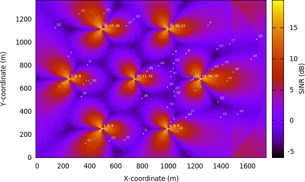
REM obtained from a simulation in handover campaign
After hours of running, the simulation campaign will eventually end. Next we will perform some post-processing on the produced simulation output to obtain meaningful information out of it.
In this example, we use GNU Octave to assist the processing of throughput and SINR data, as demonstrated in a sample GNU Octave script below:
% RxBytes is the 10th column
DlRxBytes = load ("no-op-DlRlcStats.txt") (:,10);
DlAverageThroughputKbps = sum (DlRxBytes) * 8 / 1000 / 50
% RxBytes is the 10th column
UlRxBytes = load ("no-op-UlRlcStats.txt") (:,10);
UlAverageThroughputKbps = sum (UlRxBytes) * 8 / 1000 / 50
% Sinr is the 6th column
DlSinr = load ("no-op-DlRsrpSinrStats.txt") (:,6);
% eliminate NaN values
idx = isnan (DlSinr);
DlSinr (idx) = 0;
DlAverageSinrDb = 10 * log10 (mean (DlSinr)) % convert to dB
% Sinr is the 5th column
UlSinr = load ("no-op-UlSinrStats.txt") (:,5);
% eliminate NaN values
idx = isnan (UlSinr);
UlSinr (idx) = 0;
UlAverageSinrDb = 10 * log10 (mean (UlSinr)) % convert to dB
As for the number of handovers, we can use simple shell scripting to count the number of occurrences of string “Handover” in the log file:
$ grep "Handover" no-op.txt | wc -l
Table Results of handover campaign below shows the complete statistics
after we are done with post-processing on every individual simulation run. The
values shown are the average of the results obtained from RngRun of 1, 2, 3,
and 4.
| Statistics | No-op | A2-A4-RSRQ | Strongest cell |
|---|---|---|---|
| Average DL system throughput | 6 615 kbps | 20 509 kbps | 19 709 kbps |
| Average UL system throughput | 4 095 kbps | 5 705 kbps | 6 627 kbps |
| Average DL SINR | -0.10 dB | 5.19 dB | 5.24 dB |
| Average UL SINR | 9.54 dB | 81.57 dB | 79.65 dB |
| Number of handovers per UE per second | 0 | 0.05694 | 0.04771 |
The results show that having a handover algorithm in a mobility simulation improves both user throughput and SINR significantly. There is little difference between the two handover algorithms in this campaign scenario. It would be interesting to see their performance in different scenarios, such as scenarios with home eNodeBs deployment.
Frequency Reuse examples
There are two examples showing Frequency Reuse Algorithms functionality.
lena-frequency-reuse is simple example with 3 eNBs in triangle layout.
There are 3 cell edge UEs, which are located in the center of this triangle and
3 cell center UEs (one near each eNB). User can also specify the number of randomly
located UEs. FR algorithm is installed in eNBs and each eNB has different FrCellTypeId,
what means each eNB uses different FR configuration. User can run lena-frequency-reuse
with 6 different FR algorithms: NoOp, Hard FR, Strict FR, Soft FR, Soft FFR and Enhanced FFR.
To run scenario with Distributed FFR algorithm, user should use lena-distributed-ffr.
These two examples are very similar, but they were split because Distributed FFR requires
EPC to be used, and other algorithms do not.
To run lena-frequency-reuse with different Frequency Reuse algorithms, user needs to specify
FR algorithm by overriding the default attribute ns3::LteHelper::FfrAlgorithm.
Example command to run lena-frequency-reuse with Soft FR algorithm is presented below:
$ ./waf --run "lena-frequency-reuse --ns3::LteHelper::FfrAlgorithm=ns3::LteFrSoftAlgorithm"
In these examples functionality to generate REM and spectrum analyzer trace was added.
User can enable generation of it by setting generateRem and generateSpectrumTrace
attributes.
Command to generate REM for RB 1 in data channel from lena-frequency-reuse scenario
with Soft FR algorithm is presented below:
$ ./waf --run "lena-frequency-reuse --ns3::LteHelper::FfrAlgorithm=ns3::LteFrSoftAlgorithm
--generateRem=true --remRbId=1"
Radio Environment Map for Soft FR is presented in Figure REM for RB 1 obtained from lena-frequency-reuse example with Soft FR algorithm enabled.
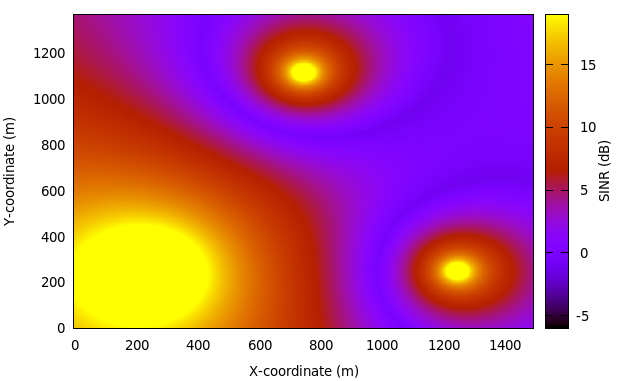
REM for RB 1 obtained from lena-frequency-reuse example with Soft FR
algorithm enabled
Command to generate spectrum trace from lena-frequency-reuse scenario
with Soft FFR algorithm is presented below (Spectrum Analyzer position needs to be configured
inside script):
$ ./waf --run "lena-frequency-reuse --ns3::LteHelper::FfrAlgorithm=ns3::LteFfrSoftAlgorithm
--generateSpectrumTrace=true"
Example spectrum analyzer trace is presented in figure Spectrum Analyzer trace obtained from lena-frequency-reuse example with Soft FFR algorithm enabled. Spectrum Analyzer was located need eNB with FrCellTypeId 2.. As can be seen, different data channel subbands are sent with different power level (according to configuration), while control channel is transmitted with uniform power along entire system bandwidth.
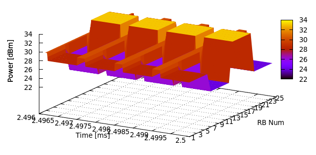
Spectrum Analyzer trace obtained from lena-frequency-reuse example
with Soft FFR algorithm enabled. Spectrum Analyzer was located need eNB
with FrCellTypeId 2.
lena-dual-stripe can be also run with Frequency Reuse algorithms installed in all macro eNB.
User needs to specify FR algorithm by overriding the default attribute ns3::LteHelper::FfrAlgorithm.
Example command to run lena-dual-stripe with Hard FR algorithm is presented below:
$ ./waf --run="lena-dual-stripe
--simTime=50 --nBlocks=0 --nMacroEnbSites=7 --nMacroEnbSitesX=2
--epc=1 --useUdp=0 --outdoorUeMinSpeed=16.6667 --outdoorUeMaxSpeed=16.6667
--ns3::LteHelper::HandoverAlgorithm=ns3::NoOpHandoverAlgorithm
--ns3::LteHelper::FfrAlgorithm=ns3::LteFrHardAlgorithm
--ns3::RadioBearerStatsCalculator::DlRlcOutputFilename=no-op-DlRlcStats.txt
--ns3::RadioBearerStatsCalculator::UlRlcOutputFilename=no-op-UlRlcStats.txt
--ns3::PhyStatsCalculator::DlRsrpSinrFilename=no-op-DlRsrpSinrStats.txt
--ns3::PhyStatsCalculator::UlSinrFilename=no-op-UlSinrStats.txt
--RngRun=1" > no-op.txt
Example command to generate REM for RB 1 in data channel from lena-dual-stripe scenario
with Hard FR algorithm is presented below:
$ ./waf --run="lena-dual-stripe
--simTime=50 --nBlocks=0 --nMacroEnbSites=7 --nMacroEnbSitesX=2
--epc=0 --useUdp=0 --outdoorUeMinSpeed=16.6667 --outdoorUeMaxSpeed=16.6667
--ns3::LteHelper::HandoverAlgorithm=ns3::NoOpHandoverAlgorithm
--ns3::LteHelper::FfrAlgorithm=ns3::LteFrHardAlgorithm
--ns3::RadioBearerStatsCalculator::DlRlcOutputFilename=no-op-DlRlcStats.txt
--ns3::RadioBearerStatsCalculator::UlRlcOutputFilename=no-op-UlRlcStats.txt
--ns3::PhyStatsCalculator::DlRsrpSinrFilename=no-op-DlRsrpSinrStats.txt
--ns3::PhyStatsCalculator::UlSinrFilename=no-op-UlSinrStats.txt
--RngRun=1 --generateRem=true --remRbId=1" > no-op.txt
Radio Environment Maps for RB 1, 10 and 20 generated from lena-dual-stripe
scenario with Hard Frequency Reuse algorithm are presented in the figures
below. These RB were selected because each one is used by different FR cell type.
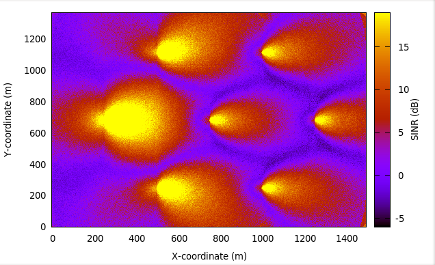
REM for RB 1 obtained from lena-dual-stripe simulation with Hard FR algorithm enabled
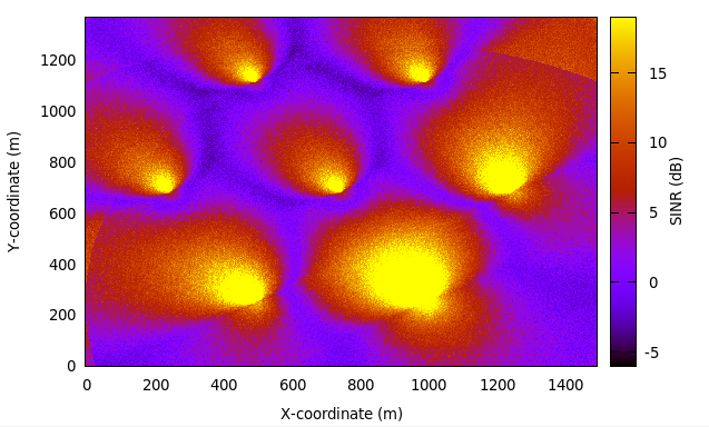
REM for RB 10 obtained from lena-dual-stripe simulation with Hard FR algorithm enabled
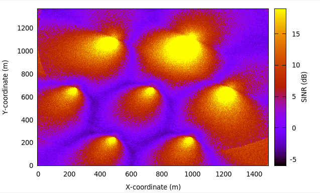
REM for RB 20 obtained from lena-dual-stripe simulation with Hard FR algorithm enabled
Carrier aggregation examples
The carrier aggregation feature is not enabled by default. The user can enable it by setting the boolean attribute
ns3::LteHelper::UseCa to true. The number of component carriers to be used in carrier aggregation can
be configured by setting the attribute ns3::LteHelper::NumberOfComponentCarriers. Currently the
maximum number is 5. Additionally, the component carrier manager needs to be configured. By default
the NoOpComponentCarrierManager is selected, which means that only the primary carrier is enabled. The Component
carrier manager (CCM) implementation that uses all the available carriers is RrComponentCarrierManager.
The CCM can be configured by using the attribute LteHelper::EnbComponentCarrierManager.
An example configuration is presented below:
Config::SetDefault ("ns3::LteHelper::UseCa", BooleanValue (useCa));
Config::SetDefault ("ns3::LteHelper::NumberOfComponentCarriers", UintegerValue (2));
Config::SetDefault ("ns3::LteHelper::EnbComponentCarrierManager", StringValue ("ns3::RrComponentCarrierManager"));
As an example, the user can take a look and run the lena-simple and lena-simple-epc programs and enable LTE traces
to check the performance. A new column is added to PHY and MAC traces to indicate the component carrier.
The test suite lte-carrier-aggregation is also a test program that can be used as an example as it can be run in a mode to write results
to output files by setting the s_writeResults boolean static variable to true. The test can be run by using a test-runner:
./waf –run ‘test-runner –suite=lte-carrier-aggregation’
To plot the test results, a file has to be created in the root folder of the ns-3 repository, and added to it with the following content :
set terminal png set xlabel “Number of users” set ylabel “Throughput per UE [Mbps]” set key top right
downlink_results=”carrier_aggregation_results_dl.txt” uplink_results=”carrier_aggregation_results_ul.txt”
set output “ca-test-example-dl.png” set title “Downlink performance”
- plot downlink_results using 1:($2==1 ? $3/1000000 : 1/0) w lp t ‘NO SDL’, \
- downlink_results using 1:($2==2 ? $3/1000000 : 1/0) w lp t ‘RR SDL 1’, downlink_results using 1:($2==3 ? $3/1000000 : 1/0) w lp t ‘RR SDL 2’
set output “ca-test-example-ul.png” set title “Uplink performance”
- plot uplink_results using 1:($2==1 ? $3/1000000 : 1/0) w lp t ‘NO SDL’, \
- uplink_results using 1:($2==2 ? $3/1000000 : 1/0) w lp t ‘RR SDL 1’, uplink_results using 1:($2==3 ? $3/1000000 : 1/0) w lp t ‘RR SDL 2’
gnuplot can be run by providing the file name, so that in the ns-3 root directory
figures are generated. An example to run this test suite is shown in figures:
fig-ca-test-example-ul and fig-ca-test-example-dl.
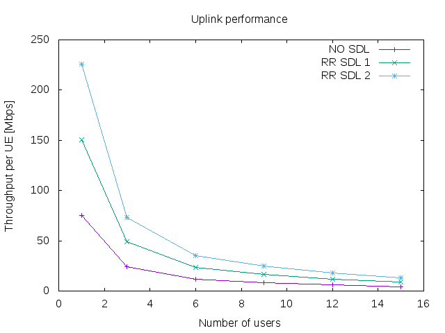
Example of CA test performance in the uplink
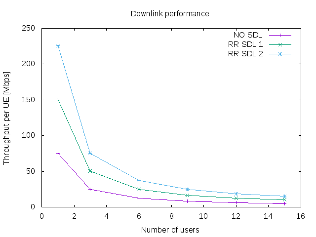
Example of CA test performance in the downlink
Radio link failure example
The example lena-radio-link-failure.cc is an example to simulate the RLF functionality. In particular, it simulates only one moving UE using Ideal or Real RRC protocol with EPC performing downlink and uplink communication in two scenarios shown in Scenario A: Radio link failure example with one eNB and Scenario B: Radio link failure example with two eNBs
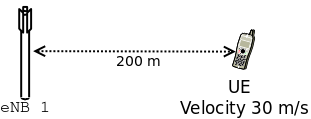
Scenario A: Radio link failure example with one eNB
We note that, the RLF detection is enabled by default, which can be disabled by
configuring the LteUePhy::EnableRlfDetection to false, e.g.,:
Config::SetDefault ("ns3::LteUePhy::EnableRlfDetection", BooleanValue (false));
In this example, to study the impact of a RLF on the user’s quality of experience, we compute an instantaneous (i.e., every 200 ms) DL throughput of the UE, and writes it into a file for plotting purposes. For example, to simulate the “Scenario A” with Ideal and Real RRC protocol a user can use the following commands:
Ideal RRC:
./waf --run "lena-radio-link-failure
--numberOfEnbs=1 --useIdealRrc=1
--interSiteDistance=1200 --n310=1 --n311=1
--t310=1 --enableCtrlErrorModel=1
--enableDataErrorModel=1 --simTime=25"
Real RRC:
./waf --run "lena-radio-link-failure
--numberOfEnbs=1 --useIdealRrc=0
--interSiteDistance=1200 --n310=1 --n311=1
--t310=1 --enableCtrlErrorModel=1
--enableDataErrorModel=1 --simTime=25"
After running the above two commands, we can use a simple gnuplot script to plot the throughput as shown in the Figure Downlink instantaneous throughput of UE in scenario A , e.g.,
set terminal png
set output "lena-radio-link-failure-one-enb-thrput.png"
set multiplot
set xlabel "Time [s]"
set ylabel "Instantaneous throughput UE [Mbps]"
set grid
set title "LTE RLF example 1 eNB DL instantaneous throughput"
plot "rlf_dl_thrput_1_eNB_ideal_rrc" using ($1):($2) with linespoints
title 'Ideal RRC' linestyle 1 lw 2 lc rgb 'blue', "rlf_dl_thrput_1_eNB_real_rrc"
using ($1):($2) with linespoints title 'Real RRC' linestyle 2 lw 2 lc rgb 'red'
unset multiplot
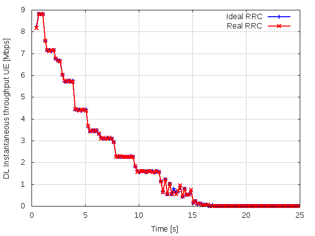
Downlink instantaneous throughput of UE in scenario A
In the simulator, a UE can synchronize (i.e., start reading system information) with an eNB at a low RSRP level, which defaults to -140 dBm (see QRxLevMin attribute of eNB RRC). It enables the UE to start the random access procedure with the eNB. In this scenario, when using the Ideal RRC the UE after the RLF will connect and disconnect from the eNB several times. This is because in the Ideal RRC mode, once the UE is able to receive Random Access Response (RAR) from the eNB, it can complete the RRC connection establishment procedure (RRC connection establishment) without any errors, since all the RRC messages are exchanged ideally between the eNB and the UE. However, soon after the connection establishment, it ends up in RLF due to the poor channel quality. On the other hand, with the Real RRC the UE after the RLF will not be able to complete the RRC connection establishment procedure due to the loss of RRC messages. Thus, it will not be able to establish the connection with the eNB. Therefore, in both the cases the UE throughput drops to zero as shown in the Figure Downlink instantaneous throughput of UE in scenario A. It is also worthwhile to mention that towards the end of the simulation (using Ideal or Real RRC) there are occasions where RAR timer at the UE MAC would timeout due to the increased distance between the eNB and the UE, which causes errors while decoding this message at the UE (Note: the downlink control error model is enabled by default).
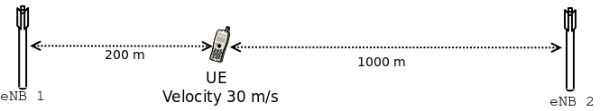
Scenario B: Radio link failure example with two eNBs
Similarly, to simulate the “Scenario B” with Ideal and Real RRC protocol following commands can be used:
Ideal RRC:
./waf --run "lena-radio-link-failure
--numberOfEnbs=2 --useIdealRrc=1
--interSiteDistance=1200 --n310=1 --n311=1
--t310=1 --enableCtrlErrorModel=1
--enableDataErrorModel=1 --simTime=25"
Real RRC:
./waf --run "lena-radio-link-failure
--numberOfEnbs=2 --useIdealRrc=0
--interSiteDistance=1200 --n310=1 --n311=1
--t310=1 --enableCtrlErrorModel=1
--enableDataErrorModel=1 --simTime=25"
Figure Downlink instantaneous throughput of UE in scenario B, shows the throughput in “Scenario B”. We note that in this scenario the handover algorithm is not used. As expected, with Ideal RRC protocol the UE after the RLF can complete the random access procedure with the second eNB. Interestingly, the DL SINR after the connection establishment is not low enough to trigger the RLF, but it is low enough to impact the DL control reception for some TBs, which in turn causes loss of data. It can be observed from the slightly unstable throughput of the UE after connecting to the second eNB. On the other hand, with Real RRC the UE faces problems in connection establishment phase due to the loss of RRC messages, in particular, the RRC connection request from the UE. This is the reason why the UE throughput after the RLF remains zero for a more extended period as compared to the ideal RRC protocol.
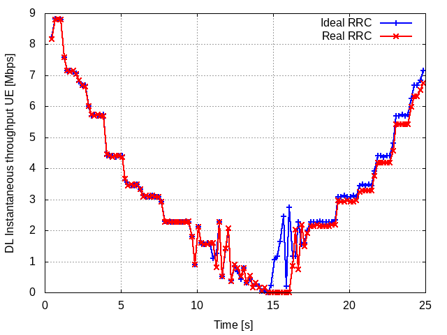
Downlink instantaneous throughput of UE in scenario B
Troubleshooting and debugging tips
Many users post on the ns-3-users mailing list asking, for example, why they do not get any traffic in their simulation, or maybe only uplink but no downlink traffic is generated, etc. In most of the cases, this is a bug in the user simulation program. Here the reader can find some tips to debug the program and find out the cause of the problem.
The general approach is to selectively and incrementally enable the logging of relevant LTE module components, verifying upon each activation that the output is as expected. In detail:
- first check the control plane, in particular the RRC connection establishment procedure, by enabling the log components LteUeRrc and LteEnbRrc
- then check packet transmissions on the data plane, starting by enabling the log components LteUeNetDevice and the EpcSgwApplication, EpcPgwApplication and EpcEnbApplication, then moving down the LTE radio stack (PDCP, RLC, MAC, and finally PHY). All this until you find where packets stop being processed / forwarded.
Testing Documentation
Overview
To test and validate the ns-3 LTE module, several test suites are provided which are integrated with the ns-3 test framework. To run them, you need to have configured the build of the simulator in this way:
$ ./waf configure --enable-tests --enable-modules=lte --enable-examples
$ ./test.py
The above will run not only the test suites belonging to the LTE module, but also those belonging to all the other ns-3 modules on which the LTE module depends. See the ns-3 manual for generic information on the testing framework.
You can get a more detailed report in HTML format in this way:
$ ./test.py -w results.html
After the above command has run, you can view the detailed result for each test by opening the file results.html with a web browser.
You can run each test suite separately using this command:
$ ./test.py -s test-suite-name
For more details about test.py and the ns-3 testing framework, please refer to the ns-3 manual.
Description of the test suites
Unit Tests
SINR calculation in the Downlink
The test suite lte-downlink-sinr
checks that the SINR calculation in
downlink is performed correctly. The SINR in the downlink is calculated for each
RB assigned to data transmissions by dividing the power of the
intended signal from the considered eNB by the sum of the noise power plus all
the transmissions on the same RB coming from other eNBs (the interference
signals):
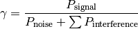
In general, different signals can be active during different periods
of time. We define a chunk as the time interval between any two
events of type either start or end of a waveform. In other words, a
chunk identifies a time interval during which the set of active
waveforms does not change. Let be the generic chunk,
 its duration and
  its SINR,
calculated with the above equation. The calculation of the average
SINR
its SINR,
calculated with the above equation. The calculation of the average
SINR  to be used for CQI feedback reporting
uses the following formula:
to be used for CQI feedback reporting
uses the following formula:

The test suite checks that the above calculation is performed
correctly in the simulator. The test vectors are obtained offline by
an Octave script that implements the above equation, and that
recreates a number of random transmitted signals and interference
signals that mimic a scenario where an UE is trying to decode a signal
from an eNB while facing interference from other eNBs. The test passes
if the calculated values are equal to the test vector within a
tolerance of  . The tolerance is meant to account for
the approximation errors typical of floating point arithmetic.
. The tolerance is meant to account for
the approximation errors typical of floating point arithmetic.
SINR calculation in the Uplink
The test suite lte-uplink-sinr checks that the SINR calculation in
uplink is performed correctly. This test suite is identical to
lte-downlink-sinr described in the previous section, with the
difference than both the signal and the interference now refer to
transmissions by the UEs, and reception is performed by the eNB.
This test suite recreates a number of random transmitted signals and
interference signals to mimic a scenario where an eNB is trying to
decode the signal from several UEs simultaneously (the ones in the
cell of the eNB) while facing interference from other UEs (the ones
belonging to other cells).
The test vectors are obtained by a dedicated Octave script. The test
passes if the calculated values are equal to the test vector within a
tolerance of which, as for the downlink SINR test,
deals with floating point arithmetic approximation issues.
E-UTRA Absolute Radio Frequency Channel Number (EARFCN)
The test suite lte-earfcn checks that the carrier frequency used
by the LteSpectrumValueHelper class (which implements the LTE spectrum
model) is done in compliance with [TS36101], where the E-UTRA
Absolute Radio Frequency Channel Number (EARFCN) is defined. The test
vector for this test suite comprises a set of EARFCN values and the
corresponding carrier frequency calculated by hand following the
specification of [TS36101]. The test passes if the carrier frequency
returned by LteSpectrumValueHelper is the same as the known value for
each element in the test vector.
System Tests
Dedicated Bearer Deactivation Tests
The test suite ‘lte-test-deactivate-bearer’ creates test case with single EnodeB and Three UE’s. Each UE consists of one Default and one Dedicated EPS bearer with same bearer specification but with different ARP. Test Case Flow is as follows: Attach UE -> Create Default+Dedicated Bearer -> Deactivate one of the Dedicated bearer
Test case further deactivates dedicated bearer having bearer ID 2(LCID=BearerId+2) of First UE (UE_ID=1) User can schedule bearer deactivation after specific time delay using Simulator::Schedule () method.
Once the test case execution ends it will create DlRlcStats.txt and UlRlcStats.txt. Key fields that need to be checked in statistics are:
|Start | end | Cell ID | IMSI | RNTI | LCID | TxBytes | RxBytes |
Test case executes in three epochs:
- In first Epoch (0.04s-1.04s) All UE’s and corresponding bearers gets attached and packet flow over the dedicated bearers activated.
- In second Epoch (1.04s-2.04s), bearer deactivation is instantiated, hence User can see relatively less number of TxBytes on UE_ID=1 and LCID=4 as compared to other bearers.
- In third Epoch (2.04s-3.04s) since bearer deactivation of UE_ID=1 and LCID=4 is completed, user will not see any logging related to LCID=4.
Test case passes if and only if
- IMSI=1 and LCID=4 completely removed in third epoch
- No packets seen in TxBytes and RxBytes corresponding to IMSI=1 and LCID=4
If above criteria do not match, the test case is considered to be failed
Adaptive Modulation and Coding Tests
The test suite lte-link-adaptation provides system tests recreating a
scenario with a single eNB and a single UE. Different test cases are created
corresponding to different SNR values perceived by the UE. The aim of the test
is to check that in each test case the chosen MCS corresponds to some known
reference values. These reference values are obtained by
re-implementing in Octave (see src/lte/test/reference/lte_amc.m) the
model described in Section Adaptive Modulation and Coding for the calculation of the
spectral efficiency, and determining the corresponding MCS index
by manually looking up the tables in [R1-081483]. The resulting test vector is
represented in Figure Test vector for Adaptive Modulation and Coding.
The MCS which is used by the simulator is measured by
obtaining the tracing output produced by the scheduler after 4ms (this
is needed to account for the initial delay in CQI reporting). The SINR
which is calculated by the simulator is also obtained using the
LteChunkProcessor interface. The test
passes if both the following conditions are satisfied:
- the SINR calculated by the simulator correspond to the SNR of the test vector within an absolute tolerance of
- the MCS index used by the simulator exactly corresponds to the one in the test vector.
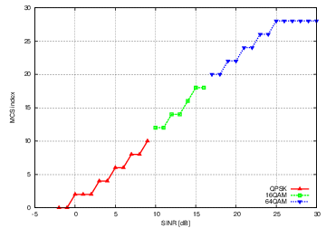
Test vector for Adaptive Modulation and Coding
Inter-cell Interference Tests
The test suite lte-interference provides system tests recreating an
inter-cell interference scenario with two eNBs, each having a single
UE attached to it and employing Adaptive Modulation and Coding both in
the downlink and in the uplink. The topology of the scenario
is depicted in Figure Topology for the inter-cell interference test. The
 parameter represents the distance of each UE to the eNB it
is attached to, whereas the
parameter represents the distance of each UE to the eNB it
is attached to, whereas the  parameter represent the
interferer distance. We note that the scenario topology is such that
the interferer distance is the same for uplink and downlink; still,
the actual interference power perceived will be different, because of
the different propagation loss in the uplink and downlink
bands. Different test cases are obtained by varying the
and parameters.
parameter represent the
interferer distance. We note that the scenario topology is such that
the interferer distance is the same for uplink and downlink; still,
the actual interference power perceived will be different, because of
the different propagation loss in the uplink and downlink
bands. Different test cases are obtained by varying the
and parameters.
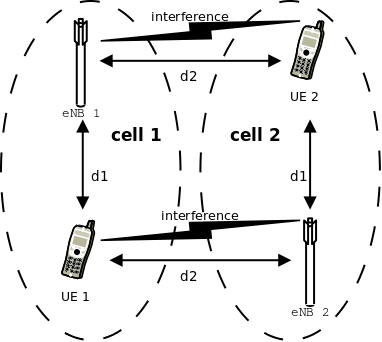
Topology for the inter-cell interference test
The test vectors are obtained by use of a dedicated octave script (available in src/lte/test/reference/lte_link_budget_interference.m), which does the link budget calculations (including interference) corresponding to the topology of each test case, and outputs the resulting SINR and spectral efficiency. The latter is then used to determine (using the same procedure adopted for Adaptive Modulation and Coding Tests. We note that the test vector contains separate values for uplink and downlink.
UE Measurements Tests
The test suite lte-ue-measurements provides system tests recreating an inter-cell interference scenario identical of the one defined for lte-interference test-suite. However, in this test the quantities to be tested are represented by RSRP and RSRQ measurements performed by the UE in two different points of the stack: the source, which is UE PHY layer, and the destination, that is the eNB RRC.
The test vectors are obtained by the use of a dedicated octave script (available in src/lte/test/reference/lte-ue-measurements.m), which does the link budget calculations (including interference) corresponding to the topology of each test case, and outputs the resulting RSRP and RSRQ. The obtained values are then used for checking the correctness of the UE Measurements at PHY layer. After that, they have to be converted according to 3GPP formatting for the purpose of checking their correctness at eNB RRC level.
UE measurement configuration tests
Besides the previously mentioned test suite, there are 3 other test suites for testing UE measurements: lte-ue-measurements-piecewise-1, lte-ue-measurements-piecewise-2, and lte-ue-measurements-handover. These test suites are more focused on the reporting trigger procedure, i.e. the correctness of the implementation of the event-based triggering criteria is verified here.
In more specific, the tests verify the timing and the content of each measurement reports received by eNodeB. Each test case is an stand-alone LTE simulation and the test case will pass if measurement report(s) only occurs at the prescribed time and shows the correct level of RSRP (RSRQ is not verified at the moment).
The piecewise configuration aims to test a particular UE measurements configuration. The simulation script will setup the corresponding measurements configuration to the UE, which will be active throughout the simulation.
Since the reference values are precalculated by hands, several assumptions are made to simplify the simulation. Firstly, the channel is only affected by path loss model (in this case, Friis model is used). Secondly, the ideal RRC protocol is used, and layer 3 filtering is disabled. Finally, the UE moves in a predefined motion pattern between 4 distinct spots, as depicted in Figure UE movement trace throughout the simulation in piecewise configuration below. Therefore the fluctuation of the measured RSRP can be determined more easily.
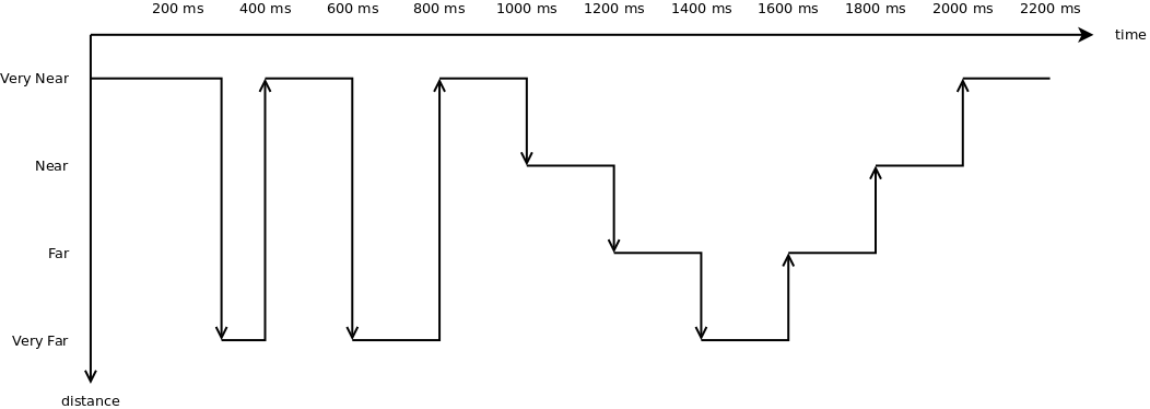
UE movement trace throughout the simulation in piecewise configuration
The motivation behind the “teleport” between the predefined spots is to introduce drastic change of RSRP level, which will guarantee the triggering of entering or leaving condition of the tested event. By performing drastic changes, the test can be run within shorter amount of time.
Figure Measured RSRP trace of an example Event A1 test case in piecewise configuration below shows the measured RSRP after layer 1 filtering by the PHY layer during the simulation with a piecewise configuration. Because layer 3 filtering is disabled, these are the exact values used by the UE RRC instance to evaluate reporting trigger procedure. Notice that the values are refreshed every 200 ms, which is the default filtering period of PHY layer measurements report. The figure also shows the time when entering and leaving conditions of an example instance of Event A1 (serving cell becomes better than threshold) occur during the simulation.
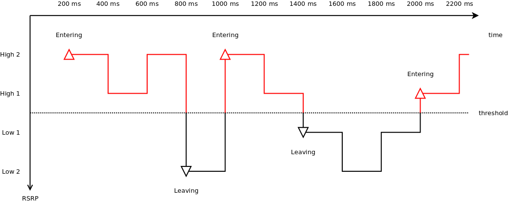
Measured RSRP trace of an example Event A1 test case in piecewise configuration
Each reporting criterion is tested several times with different threshold/offset parameters. Some test scenarios also take hysteresis and time-to-trigger into account. Figure Measured RSRP trace of an example Event A1 with hysteresis test case in piecewise configuration depicts the effect of hysteresis in another example of Event A1 test.
Measured RSRP trace of an example Event A1 with hysteresis test case in piecewise configuration
Piecewise configuration is used in two test suites of UE measurements. The first one is lte-ue-measurements-piecewise-1, henceforth Piecewise test #1, which simulates 1 UE and 1 eNodeB. The other one is lte-ue-measurements-piecewise-2, which has 1 UE and 2 eNodeBs in the simulation.
Piecewise test #1 is intended to test the event-based criteria which are not dependent on the existence of a neighboring cell. These criteria include Event A1 and A2. The other events are also briefly tested to verify that they are still working correctly (albeit not reporting anything) in the absence of any neighboring cell. Table UE measurements test scenarios using piecewise configuration #1 below lists the scenarios tested in piecewise test #1.
| Test # | Reporting Criteria | Threshold/Offset | Hysteresis | Time-to-Trigger |
|---|---|---|---|---|
| 1 | Event A1 | Low | No | No |
| 2 | Event A1 | Normal | No | No |
| 3 | Event A1 | Normal | No | Short |
| 4 | Event A1 | Normal | No | Long |
| 5 | Event A1 | Normal | No | Super |
| 6 | Event A1 | Normal | Yes | No |
| 7 | Event A1 | High | No | No |
| 8 | Event A2 | Low | No | No |
| 9 | Event A2 | Normal | No | No |
| 10 | Event A2 | Normal | No | Short |
| 11 | Event A2 | Normal | No | Long |
| 12 | Event A2 | Normal | No | Super |
| 13 | Event A2 | Normal | Yes | No |
| 14 | Event A2 | High | No | No |
| 15 | Event A3 | Zero | No | No |
| 16 | Event A4 | Normal | No | No |
| 17 | Event A5 | Normal-Normal | No | No |
Other events such as Event A3, A4, and A5 depend on measurements of neighbouring cell, so they are more thoroughly tested in Piecewise test #2. The simulation places the nodes on a straight line and instruct the UE to “jump” in a similar manner as in Piecewise test #1. Handover is disabled in the simulation, so the role of serving and neighbouring cells do not switch during the simulation. Table UE measurements test scenarios using piecewise configuration #2 below lists the scenarios tested in Piecewise test #2.
| Test # | Reporting Criteria | Threshold/Offset | Hysteresis | Time-to-Trigger |
|---|---|---|---|---|
| 1 | Event A1 | Low | No | No |
| 2 | Event A1 | Normal | No | No |
| 3 | Event A1 | Normal | Yes | No |
| 4 | Event A1 | High | No | No |
| 5 | Event A2 | Low | No | No |
| 6 | Event A2 | Normal | No | No |
| 7 | Event A2 | Normal | Yes | No |
| 8 | Event A2 | High | No | No |
| 9 | Event A3 | Positive | No | No |
| 10 | Event A3 | Zero | No | No |
| 11 | Event A3 | Zero | No | Short |
| 12 | Event A3 | Zero | No | Super |
| 13 | Event A3 | Zero | Yes | No |
| 14 | Event A3 | Negative | No | No |
| 15 | Event A4 | Low | No | No |
| 16 | Event A4 | Normal | No | No |
| 17 | Event A4 | Normal | No | Short |
| 18 | Event A4 | Normal | No | Super |
| 19 | Event A4 | Normal | Yes | No |
| 20 | Event A4 | High | No | No |
| 21 | Event A5 | Low-Low | No | No |
| 22 | Event A5 | Low-Normal | No | No |
| 23 | Event A5 | Low-High | No | No |
| 24 | Event A5 | Normal-Low | No | No |
| 25 | Event A5 | Normal-Normal | No | No |
| 26 | Event A5 | Normal-Normal | No | Short |
| 27 | Event A5 | Normal-Normal | No | Super |
| 28 | Event A5 | Normal-Normal | Yes | No |
| 29 | Event A5 | Normal-High | No | No |
| 30 | Event A5 | High-Low | No | No |
| 31 | Event A5 | High-Normal | No | No |
| 32 | Event A5 | High-High | No | No |
One note about the tests with time-to-trigger, they are tested using 3 different values of time-to-trigger: short (shorter than report interval), long (shorter than the filter measurement period of 200 ms), and super (longer than 200 ms). The first two ensure that time-to-trigger evaluation always use the latest measurement reports received from PHY layer. While the last one is responsible for verifying time-to-trigger cancellation, for example when a measurement report from PHY shows that the entering/leaving condition is no longer true before the first trigger is fired.
The purpose of the handover configuration is to verify whether UE measurement configuration is updated properly after a successful handover takes place. For this purpose, the simulation will construct 2 eNodeBs with different UE measurement configuration, and the UE will perform handover from one cell to another. The UE will be located on a straight line between the 2 eNodeBs, and the handover will be invoked manually. The duration of each simulation is 2 seconds (except the last test case) and the handover is triggered exactly at halfway of simulation.
The lte-ue-measurements-handover test suite covers various types of configuration differences. The first one is the difference in report interval, e.g. the first eNodeB is configured with 480 ms report interval, while the second eNodeB is configured with 240 ms report interval. Therefore, when the UE performed handover to the second cell, the new report interval must take effect. As in piecewise configuration, the timing and the content of each measurement report received by the eNodeB will be verified.
Other types of differences covered by the test suite are differences in event and differences in threshold/offset. Table UE measurements test scenarios using handover configuration below lists the tested scenarios.
| Test # | Test Subject | Initial Configuration | Post-Handover Configuration |
|---|---|---|---|
| 1 | Report interval | 480 ms | 240 ms |
| 2 | Report interval | 120 ms | 640 ms |
| 3 | Event | Event A1 | Event A2 |
| 4 | Event | Event A2 | Event A1 |
| 5 | Event | Event A3 | Event A4 |
| 6 | Event | Event A4 | Event A3 |
| 7 | Event | Event A2 | Event A3 |
| 8 | Event | Event A3 | Event A2 |
| 9 | Event | Event A4 | Event A5 |
| 10 | Event | Event A5 | Event A4 |
| 11 | Threshold/offset | RSRP range 52 (Event A1) | RSRP range 56 (Event A1) |
| 12 | Threshold/offset | RSRP range 52 (Event A2) | RSRP range 56 (Event A2) |
| 13 | Threshold/offset | A3 offset -30 (Event A3) | A3 offset +30 (Event A3) |
| 14 | Threshold/offset | RSRP range 52 (Event A4) | RSRP range 56 (Event A4) |
| 15 | Threshold/offset | RSRP range 52-52 (Event A5) | RSRP range 56-56 (Event A5) |
| 16 | Time-to-trigger | 1024 ms | 100 ms |
| 17 | Time-to-trigger | 1024 ms | 640 ms |
Round Robin scheduler performance
The test suite lte-rr-ff-mac-scheduler creates different test cases with
a single eNB and several UEs, all having the same Radio Bearer specification. In
each test case, the UEs see the same SINR from the eNB; different test cases are
implemented by using different distance among UEs and the eNB (i.e., therefore
having different SINR values) and different numbers of UEs. The test consists on
checking that the obtained throughput performance is equal among users and
matches a reference throughput value obtained according to the SINR perceived
within a given tolerance.
The test vector is obtained according to the values of transport block
size reported in table 7.1.7.2.1-1 of [TS36213], considering an
equal distribution of the physical resource block among the users
using Resource Allocation Type 0 as defined in Section 7.1.6.1 of
[TS36213]. Let be the TTI duration, be the
number of UEs, the transmission bandwidth configuration in
number of RBs,  the RBG size, the modulation and
coding scheme in use at the given SINR and be the
transport block size in bits as defined by 3GPP TS 36.213. We first
calculate the number
the RBG size, the modulation and
coding scheme in use at the given SINR and be the
transport block size in bits as defined by 3GPP TS 36.213. We first
calculate the number  of RBGs allocated to each user as

The reference throughput  in bit/s achieved by each UE is then calculated as
The test passes if the measured throughput matches with the reference throughput within a relative tolerance of 0.1. This tolerance is needed to account for the transient behavior at the beginning of the simulation (e.g., CQI feedback is only available after a few subframes) as well as for the accuracy of the estimator of the average throughput performance over the chosen simulation time (0.4s). This choice of the simulation time is justified by the need to follow the ns-3 guidelines of keeping the total execution time of the test suite low, in spite of the high number of test cases. In any case, we note that a lower value of the tolerance can be used when longer simulations are run.
In Figure fig-lenaThrTestCase1, the curves labeled “RR” represent the test values calculated for the RR scheduler test, as a function of the number of UEs and of the MCS index being used in each test case.
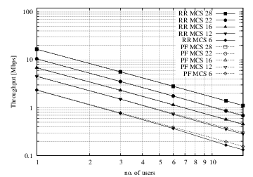
Test vectors for the RR and PF Scheduler in the downlink in a scenario where all UEs use the same MCS.
Proportional Fair scheduler performance
The test suite lte-pf-ff-mac-scheduler creates different test cases with
a single eNB, using the Proportional Fair (PF) scheduler, and several UEs, all
having the same Radio Bearer specification. The test cases are grouped in two
categories in order to evaluate the performance both in terms of the adaptation
to the channel condition and from a fairness perspective.
In the first category of test cases, the UEs are all placed at the
same distance from the eNB, and hence all placed in order to have the
same SINR. Different test cases are implemented by using a different
SINR value and a different number of UEs. The test consists on
checking that the obtained throughput performance matches with the
known reference throughput up to a given tolerance. The expected
behavior of the PF scheduler when all UEs have the same SNR is that
each UE should get an equal fraction of the throughput obtainable by a
single UE when using all the resources. We calculate the reference
throughput value by dividing the throughput achievable by a single UE
at the given SNR by the total number of UEs.
Let be the TTI duration, the transmission
bandwidth configuration in number of RBs, the modulation and
coding scheme in use at the given SINR and be the
transport block size as defined in [TS36213]. The reference
throughput in bit/s achieved by each UE is calculated as
The curves labeled “PF” in Figure fig-lenaThrTestCase1 represent the test values calculated for the PF scheduler tests of the first category, that we just described.
The second category of tests aims at verifying the fairness of the PF
scheduler in a more realistic simulation scenario where the UEs have a
different SINR (constant for the whole simulation). In these conditions, the PF
scheduler will give to each user a share of the system bandwidth that is
proportional to the capacity achievable by a single user alone considered its
SINR. In detail, let be the modulation and coding scheme being used by
each UE (which is a deterministic function of the SINR of the UE, and is hence
known in this scenario). Based on the MCS, we determine the achievable
rate  for each user using the
procedure described in Section~ref{sec:pfs}. We then define the
achievable rate ratio
for each user using the
procedure described in Section~ref{sec:pfs}. We then define the
achievable rate ratio  of each user as
Let now be the throughput actually achieved by the UE , which
is obtained as part of the simulation output. We define the obtained throughput
ratio  of UE as
The test consists of checking that the following condition is verified:

if so, it means that the throughput obtained by each UE over the whole simulation matches with the steady-state throughput expected by the PF scheduler according to the theory. This test can be derived from [Holtzman2000] as follows. From Section 3 of [Holtzman2000], we know that

where is a constant. By substituting the above into the
definition of given previously, we get
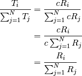
which is exactly the expression being used in the test.
Figure Throughput ratio evaluation for the PF scheduler in a scenario
where the UEs have MCS index 28, 24, 16, 12, 6 presents the results obtained in a test case with
UEs  that are located at a distance from the base
station such that they will use respectively the MCS index
that are located at a distance from the base
station such that they will use respectively the MCS index  . From the figure, we note that, as expected, the obtained throughput is
proportional to the achievable rate. In other words, the PF scheduler assign
more resources to the users that use a higher MCS index.
. From the figure, we note that, as expected, the obtained throughput is
proportional to the achievable rate. In other words, the PF scheduler assign
more resources to the users that use a higher MCS index.
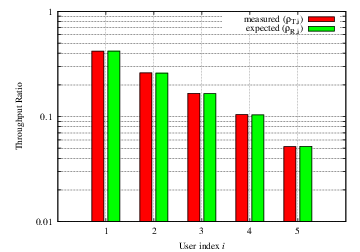
Throughput ratio evaluation for the PF scheduler in a scenario
where the UEs have MCS index 
Maximum Throughput scheduler performance
Test suites lte-fdmt-ff-mac-scheduler and lte-tdmt-ff-mac-scheduler
create different test cases with a single eNB and several UEs, all having the same
Radio Bearer specification, using the Frequency Domain Maximum Throughput (FDMT)
scheduler and Time Domain Maximum Throughput (TDMT) scheduler respectively.
In other words, UEs are all placed at the
same distance from the eNB, and hence all placed in order to have the
same SNR. Different test cases are implemented by using a different
SNR values and a different number of UEs. The test consists on
checking that the obtained throughput performance matches with the
known reference throughput up to a given tolerance.The expected
behavior of both FDMT and TDMT scheduler when all UEs have the same SNR is that
scheduler allocates all RBGs to the first UE defined in script. This is because
the current FDMT and TDMT implementation always select the first UE to serve when there are
multiple UEs having the same SNR value. We calculate the reference
throughput value for first UE by the throughput achievable of a single UE
at the given SNR, while reference throughput value for other UEs by zero.
Let be the TTI duration, the transmission
bandwidth configuration in number of RBs, the modulation and
coding scheme in use at the given SNR and be the
transport block size as defined in [TS36213]. The reference
throughput in bit/s achieved by each UE is calculated as
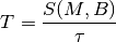
Throughput to Average scheduler performance
Test suites lte-tta-ff-mac-scheduler
create different test cases with a single eNB and several UEs, all having the same
Radio Bearer specification using TTA scheduler. Network topology and configurations in
TTA test case are as the same as the test for MT scheduler. More complex test case needs to be
developed to show the fairness feature of TTA scheduler.
Blind Average Throughput scheduler performance
Test suites lte-tdbet-ff-mac-scheduler and lte-fdbet-ff-mac-scheduler create different
test cases with a single eNB and several UEs, all having the same Radio Bearer specification.
In the first test case of lte-tdbet-ff-mac-scheduler and lte-fdbet-ff-mac-scheduler,
the UEs are all placed at the same distance from the eNB, and hence all placed in order to
have the same SNR. Different test cases are implemented by using a different SNR value and
a different number of UEs. The test consists on checking that the obtained throughput performance
matches with the known reference throughput up to a given tolerance. In long term, the expected
behavior of both TD-BET and FD-BET when all UEs have the same SNR is that each UE should get an
equal throughput. However, the exact throughput value of TD-BET and FD-BET in this test case is not
the same.
When all UEs have the same SNR, TD-BET can be seen as a specific case of PF where achievable rate equals to 1. Therefore, the throughput obtained by TD-BET is equal to that of PF. On the other hand, FD-BET performs very similar to the round robin (RR) scheduler in case of that all UEs have the same SNR and the number of UE( or RBG) is an integer multiple of the number of RBG( or UE). In this case, FD-BET always allocate the same number of RBGs to each UE. For example, if eNB has 12 RBGs and there are 6 UEs, then each UE will get 2 RBGs in each TTI. Or if eNB has 12 RBGs and there are 24 UEs, then each UE will get 2 RBGs per two TTIs. When the number of UE (RBG) is not an integer multiple of the number of RBG (UE), FD-BET will not follow the RR behavior because it will assigned different number of RBGs to some UEs, while the throughput of each UE is still the same.
The second category of tests aims at verifying the fairness of the both TD-BET and FD-BET schedulers in a more realistic simulation scenario where the UEs have a different SNR (constant for the whole simulation). In this case, both scheduler should give the same amount of averaged throughput to each user.
Specifically, for TD-BET, let  be the fraction of time allocated to user i in total simulation time,
 be the full bandwidth achievable rate for user i and be the achieved throughput of
user i. Then we have:
be the full bandwidth achievable rate for user i and be the achieved throughput of
user i. Then we have:

In TD-BET, the sum of for all user equals one. In long term, all UE has the same so that we replace
by . Then we have:
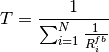
Token Band Fair Queue scheduler performance
Test suites lte-fdtbfq-ff-mac-scheduler and lte-tdtbfq-ff-mac-scheduler create different
test cases for testing three key features of TBFQ scheduler: traffic policing, fairness and traffic
balance. Constant Bit Rate UDP traffic is used in both downlink and uplink in all test cases.
The packet interval is set to 1ms to keep the RLC buffer non-empty. Different traffic rate is
achieved by setting different packet size. Specifically, two classes of flows are created in the
test suites:
- Homogeneous flow: flows with the same token generation rate and packet arrival rate
- Heterogeneous flow: flows with different packet arrival rate, but with the same token generation rate
In test case 1 verifies traffic policing and fairness features for the scenario that all UEs are placed at the same distance from the eNB. In this case, all Ues have the same SNR value. Different test cases are implemented by using a different SNR value and a different number of UEs. Because each flow have the same traffic rate and token generation rate, TBFQ scheduler will guarantee the same throughput among UEs without the constraint of token generation rate. In addition, the exact value of UE throughput is depended on the total traffic rate:
- If total traffic rate <= maximum throughput, UE throughput = traffic rate
- If total traffic rate > maximum throughput, UE throughput = maximum throughput / N
Here, N is the number of UE connected to eNodeB. The maximum throughput in this case equals to the rate that all RBGs are assigned to one UE(e.g., when distance equals 0, maximum throughput is 2196000 byte/sec). When the traffic rate is smaller than max bandwidth, TBFQ can police the traffic by token generation rate so that the UE throughput equals its actual traffic rate (token generation rate is set to traffic generation rate); On the other hand, when total traffic rate is bigger than the max throughput, eNodeB cannot forward all traffic to UEs. Therefore, in each TTI, TBFQ will allocate all RBGs to one UE due to the large packets buffered in RLC buffer. When a UE is scheduled in current TTI, its token counter is decreased so that it will not be scheduled in the next TTI. Because each UE has the same traffic generation rate, TBFQ will serve each UE in turn and only serve one UE in each TTI (both in TD TBFQ and FD TBFQ). Therefore, the UE throughput in the second condition equals to the evenly share of maximum throughput.
Test case 2 verifies traffic policing and fairness features for the scenario that each UE is placed at the different distance from the eNB. In this case, each UE has the different SNR value. Similar to test case 1, UE throughput in test case 2 is also depended on the total traffic rate but with a different maximum throughput. Suppose all UEs have a high traffic load. Then the traffic will saturate the RLC buffer in eNodeB. In each TTI, after selecting one UE with highest metric, TBFQ will allocate all RBGs to this UE due to the large RLC buffer size. On the other hand, once RLC buffer is saturated, the total throughput of all UEs cannot increase any more. In addition, as we discussed in test case 1, for homogeneous flows which have the same t_i and r_i, each UE will achieve the same throughput in long term. Therefore, we can use the same method in TD BET to calculate the maximum throughput:

Here, is the maximum throughput. be the full bandwidth achievable rate
for user i. is the number of UE.
When the total traffic rate is bigger than , the UE throughput equals to  . Otherwise, UE throughput
equals to its traffic generation rate.
. Otherwise, UE throughput
equals to its traffic generation rate.
In test case 3, three flows with different traffic rate are created. Token generation rate for each flow is the same and equals to the average traffic rate of three flows. Because TBFQ use a shared token bank, tokens contributed by UE with lower traffic load can be utilized by UE with higher traffic load. In this way, TBFQ can guarantee the traffic rate for each flow. Although we use heterogeneous flow here, the calculation of maximum throughput is as same as that in test case 2. In calculation max throughput of test case 2, we assume that all UEs suffer high traffic load so that scheduler always assign all RBGs to one UE in each TTI. This assumes is also true in heterogeneous flow case. In other words, whether those flows have the same traffic rate and token generation rate, if their traffic rate is bigger enough, TBFQ performs as same as it in test case 2. Therefore, the maximum bandwidth in test case 3 is as same as it in test case 2.
In test case 3, in some flows, token generate rate does not equal to MBR, although all flows are CBR traffic. This is not accorded with our parameter setting rules. Actually, the traffic balance feature is used in VBR traffic. Because different UE’s peak rate may occur in different time, TBFQ use shared token bank to balance the traffic among those VBR traffics. Test case 3 use CBR traffic to verify this feature. But in the real simulation, it is recommended to set token generation rate to MBR.
Priority Set scheduler performance
Test suites lte-pss-ff-mac-scheduler create different test cases with a single eNB and several UEs.
In all test cases, we select PFsch in FD scheduler. Same testing results can also be obtained by using CoItA
scheduler. In addition, all test cases do not define nMux so that TD scheduler in PSS will always select half
of total UE.
In the first class test case of lte-pss-ff-mac-scheduler, the UEs are all placed at the same distance from
the eNB, and hence all placed in order to have the same SNR. Different test cases are implemented
by using a different TBR for each UEs. In each test cases, all UEs have the same
Target Bit Rate configured by GBR in EPS bear setting. The expected behavior of PSS is to guarantee that
each UE’s throughput at least equals its TBR if the total flow rate is blow maximum throughput. Similar
to TBFQ, the maximum throughput in this case equals to the rate that all RBGs are assigned to one UE.
When the traffic rate is smaller than max bandwidth, the UE throughput equals its actual traffic rate;
On the other hand, UE throughput equals to the evenly share of the maximum throughput.
In the first class of test cases, each UE has the same SNR. Therefore, the priority metric in PF scheduler will be
determined by past average throughput because each UE has the same achievable throughput
 in PFsch or same
 ![CoI[k,n]](_images/math/ec000409102d58823e10806d15dba99d0b2e18d3.png) in CoItA. This means that PSS will performs like a
TD-BET which allocates all RBGs to one UE in each TTI. Then the maximum value of UE throughput equals to
the achievable rate that all RBGs are allocated to this UE.
in CoItA. This means that PSS will performs like a
TD-BET which allocates all RBGs to one UE in each TTI. Then the maximum value of UE throughput equals to
the achievable rate that all RBGs are allocated to this UE.
In the second class of test case of lte-pss-ff-mac-scheduler, the UEs are all placed at the same distance from
the eNB, and hence all placed in order to have the same SNR. Different TBR values are assigned to each UE.
There also exist an maximum throughput in this case. Once total traffic rate is bigger than this threshold,
there will be some UEs that cannot achieve their TBR. Because there is no fading, subband CQIs for each
RBGs frequency are the same. Therefore, in FD scheduler,in each TTI, priority metrics of UE for all RBGs
are the same. This means that FD scheduler will always allocate all RBGs to one user. Therefore, in the
maximum throughput case, PSS performs like a TD-BET. Then we have:
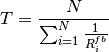
Here, is the maximum throughput. be the full bandwidth achievable rate
for user i. is the number of UE.
Channel and QoS aware scheduler performance
The performance of the Channel and QoS aware scheduler can be tested in the similar way to performance of
Priority Set scheduler when GBR flows are not delay sensitive by measuring if the achieved throughput at
RLC layer is close to the TBR. Having this in mind, the performance of the CQA scheduler is tested by using
the same test cases as the lte-pss-ff-mac-scheduler. Additionally, in [Bbojovic2014] can be found performance
evaluation of CQA scheduler when the GBR flows are delay sensitive by considering different QoE metrics.
Building Propagation Loss Model
The aim of the system test is to verify the integration of the
BuildingPathlossModel with the lte module. The test exploits a set of
three pre calculated losses for generating the expected SINR at the
receiver counting the transmission and the noise powers. These SINR
values are compared with the results obtained from a LTE
simulation that uses the BuildingPathlossModel. The reference loss values are
calculated off-line with an Octave script
(/test/reference/lte_pathloss.m). Each test case passes if the
reference loss value is equal to the value calculated by the simulator
within a tolerance of  dB, which accounts for numerical
errors in the calculations.
dB, which accounts for numerical
errors in the calculations.
Physical Error Model
The test suite lte-phy-error-model generates different test cases for
evaluating both data and control error models. For what concern the data, the
test consists of six test cases with single eNB and a various number of UEs,
all having the same Radio Bearer specification. Each test is designed for
evaluating the error rate perceived by a specific TB size in order to verify
that it corresponds to the expected values according to the BLER generated for
CB size analog to the TB size. This means that, for instance, the test will
check that the performance of a TB of bits is analogous to the one of
a CB size of bits by collecting the performance of a user which has
been forced the generation of a such TB size according to the distance to eNB.
In order to significantly test the BLER at MAC level, we configured the Adaptive
Modulation and Coding (AMC) module, the LteAmc class, for making it less
robust to channel conditions by using the PiroEW2010 AMC model and configuring
it to select the MCS considering a target BER of 0.03 (instead of the default
value of 0.00005). We note that these values do not reflect the actual BER,
since they come from an analytical bound which does not consider all the
transmission chain aspects; therefore the BER and BLER actually experienced at
the reception of a TB is in general different.
The parameters of the six test cases are reported in the following:
- 4 UEs placed 1800 meters far from the eNB, which implies the use of MCS 2 (SINR of -5.51 dB) and a TB of 256 bits, that in turns produce a BLER of 0.33 (see point A in figure BLER for tests 1, 2, 3.).
- 2 UEs placed 1800 meters far from the eNB, which implies the use of MCS 2 (SINR of -5.51 dB) and a TB of 528 bits, that in turns produce a BLER of 0.11 (see point B in figure BLER for tests 1, 2, 3.).
- 1 UE placed 1800 meters far from the eNB, which implies the use of MCS 2 (SINR of -5.51 dB) and a TB of 1088 bits, that in turns produce a BLER of 0.02 (see point C in figure BLER for tests 1, 2, 3.).
- 1 UE placed 600 meters far from the eNB, which implies the use of MCS 12 (SINR of 4.43 dB) and a TB of 4800 bits, that in turns produce a BLER of 0.3 (see point D in figure BLER for tests 4, 5.).
- 3 UEs placed 600 meters far from the eNB, which implies the use of MCS 12 (SINR of 4.43 dB) and a TB of 1632 bits, that in turns produce a BLER of 0.55 (see point E in figure BLER for tests 4, 5.).
- 1 UE placed 470 meters far from the eNB, which implies the use of MCS 16 (SINR of 8.48 dB) and a TB of 7272 bits (segmented in 2 CBs of 3648 and 3584 bits), that in turns produce a BLER of 0.14, since each CB has CBLER equal to 0.075 (see point F in figure BLER for test 6.).
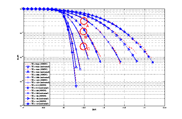
BLER for tests 1, 2, 3.
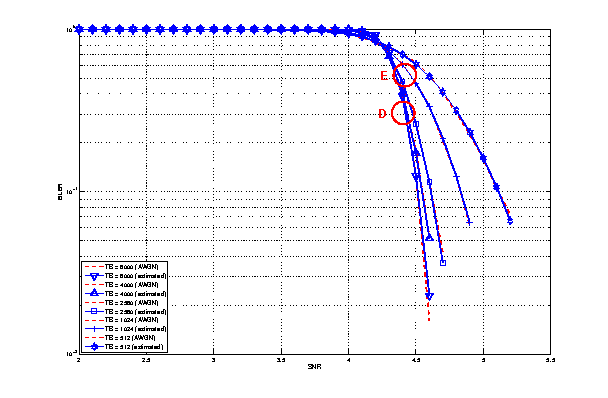
BLER for tests 4, 5.
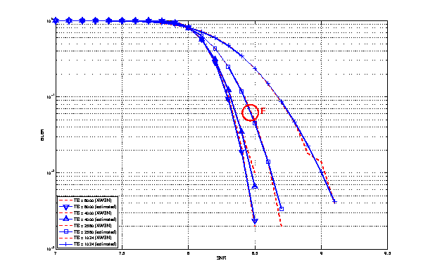
BLER for test 6.
The test condition verifies that in each test case the expected number of
packets received correctly corresponds to a Bernoulli distribution with a
confidence interval of 99%, where the probability of success in each trail is
 and is the total number of packets sent.
The error model of PCFICH-PDCCH channels consists of 4 test cases with a single UE and several eNBs, where the UE is connected to only one eNB in order to have the remaining acting as interfering ones. The errors on data are disabled in order to verify only the ones due to erroneous decodification of PCFICH-PDCCH. As before, the system has been forced on working in a less conservative fashion in the AMC module for appreciating the results in border situations. The parameters of the 4 tests cases are reported in the following:
- 2 eNBs placed 1078 meters far from the UE, which implies a SINR of -2.00 dB and a TB of 217 bits, that in turns produce a BLER of 0.007.
- 3 eNBs placed 1040 meters far from the UE, which implies a SINR of -4.00 dB and a TB of 217 bits, that in turns produce a BLER of 0.045.
- 4 eNBs placed 1250 meters far from the UE, which implies a SINR of -6.00 dB and a TB of 133 bits, that in turns produce a BLER of 0.206.
- 5 eNBs placed 1260 meters far from the UE, which implies a SINR of -7.00 dB and a TB of 81 bits, that in turns produce a BLER of 0.343.
The test condition verifies that in each test case the expected number
of packets received correct corresponds to a Bernoulli distribution
with a confidence interval of 99.8%, where the probability of success
in each trail is and is the total number of
packet sent. The larger confidence interval is due to the errors that
might be produced in quantizing the MI and the error curve.
HARQ Model
The test suite lte-harq includes two tests for evaluating the HARQ model and the related extension in the error model. The test consists on checking whether the amount of bytes received during the simulation corresponds to the expected ones according to the values of transport block and the HARQ dynamics. In detail, the test checks whether the throughput obtained after one HARQ retransmission is the expected one. For evaluating the expected throughput the expected TB delivering time has been evaluated according to the following formula:

where  is the probability of receiving with success the HARQ block at the attempt (i.e., the RV with 3GPP naming). According to the scenarios, in the test we always have
  equal to 0.0, while
  varies in the two tests, in detail:
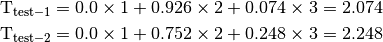
The expected throughput is calculted by counting the number of transmission slots available during the simulation (e.g., the number of TTIs) and the size of the TB in the simulation, in detail:

where  is the total number of TTIs in 1 second.
The test is performed both for Round Robin scheduler. The test passes if the measured throughput matches with the reference throughput within a relative tolerance of 0.1. This tolerance is needed to account for the transient behavior at the beginning of the simulation and the on-fly blocks at the end of the simulation.
is the total number of TTIs in 1 second.
The test is performed both for Round Robin scheduler. The test passes if the measured throughput matches with the reference throughput within a relative tolerance of 0.1. This tolerance is needed to account for the transient behavior at the beginning of the simulation and the on-fly blocks at the end of the simulation.
MIMO Model
The test suite lte-mimo aims at verifying both the effect of the gain considered for each Transmission Mode on the system performance and the Transmission Mode switching through the scheduler interface. The test consists on checking whether the amount of bytes received during a certain window of time (0.1 seconds in our case) corresponds to the expected ones according to the values of transport block
size reported in table 7.1.7.2.1-1 of [TS36213], similarly to what done for the tests of the schedulers.
The test is performed both for Round Robin and Proportional Fair schedulers. The test passes if the measured throughput matches with the reference throughput within a relative tolerance of 0.1. This tolerance is needed to account for the transient behavior at the beginning of the simulation and the transition phase between the Transmission Modes.
Antenna Model integration
The test suite lte-antenna checks that the AntennaModel integrated
with the LTE model works correctly. This test suite recreates a
simulation scenario with one eNB node at coordinates (0,0,0) and one
UE node at coordinates (x,y,0). The eNB node is configured with an
CosineAntennaModel having given orientation and beamwidth. The UE
instead uses the default IsotropicAntennaModel. The test
checks that the received power both in uplink and downlink account for
the correct value of the antenna gain, which is determined
offline; this is implemented by comparing the uplink and downlink SINR
and checking that both match with the reference value up to a
tolerance of  which accounts for numerical errors.
Different test cases are provided by varying the x and y coordinates
of the UE, and the beamwidth and the orientation of the antenna of
the eNB.
which accounts for numerical errors.
Different test cases are provided by varying the x and y coordinates
of the UE, and the beamwidth and the orientation of the antenna of
the eNB.
RLC
Two test suites lte-rlc-um-transmitter and
lte-rlc-am-transmitter check that the UM RLC and the AM RLC
implementation work correctly. Both these suites work by testing RLC
instances connected to special test entities that play the role of the
MAC and of the PDCP, implementing respectively the LteMacSapProvider
and LteRlcSapUser interfaces. Different test cases (i.e., input test
vector consisting of series of primitive calls by the MAC and the
PDCP) are provided that check the behavior in the following cases:
- one SDU, one PDU: the MAC notifies a TX opportunity causes the creation of a PDU which exactly contains a whole SDU
- segmentation: the MAC notifies multiple TX opportunities that are smaller than the SDU size stored in the transmission buffer, which is then to be fragmented and hence multiple PDUs are generated;
- concatenation: the MAC notifies a TX opportunity that is bigger than the SDU, hence multiple SDUs are concatenated in the same PDU
- buffer status report: a series of new SDUs notifications by the PDCP is inteleaved with a series of TX opportunity notification in order to verify that the buffer status report procedure is correct.
In all these cases, an output test vector is determine manually from knowledge of the input test vector and knowledge of the expected behavior. These test vector are specialized for UM RLC and AM RLC due to their different behavior. Each test case passes if the sequence of primitives triggered by the RLC instance being tested is exactly equal to the output test vector. In particular, for each PDU transmitted by the RLC instance, both the size and the content of the PDU are verified to check for an exact match with the test vector.
The AM RLC implementation features an additional test suite,
lte-rlc-am-e2e, which test the correct retransmission of RLC PDUs
in presence of channel losses. The test instantiates an RLC AM
transmitter and a receiver, and interposes a channel that randomly
drops packet according to a fixed loss probability. Different test
cases are instantiated using different RngRun values and different
loss probability values. Each test case passes if at the end of the
simulation all SDUs are correctly delivered to the upper layers of the
receiving RLC AM entity.
RRC
The test suite lte-rrc tests the correct functionality of the following aspects:
- MAC Random Access
- RRC System Information Acquisition
- RRC Connection Establishment
- RRC Reconfiguration
The test suite considers a type of scenario with four eNBs aligned in a square layout with 100-meter edges. Multiple UEs are located at a specific spot on the diagonal of the square and are instructed to connect to the first eNB. Each test case implements an instance of this scenario with specific values of the following parameters:
- number of UEs
- number of Data Radio Bearers to be activated for each UE
- time
at which the first UE is instructed to start connecting to the eNB
- time interval
between the start of connection of UE
; the time at which user
sdf
- the relative position of the UEs on the diagonal of the square, where higher values indicate larger distance from the serving eNodeB, i.e., higher interference from the other eNodeBs
- a boolean flag indicating whether the ideal or the real RRC protocol model is used
Each test cases passes if a number of test conditions are positively evaluated for each UE after a delay  from the time it started connecting to the eNB. The delay is determined as

where:
is the max delay necessary for the acquisition of System Information. We set it to 90ms accounting for 10ms for the MIB acquisition and 80ms for the subsequent SIB2 acquisition
is the delay for the MAC Random Access (RA) procedure. This depends on preamble collisions as well as on the availability of resources for the UL grant allocation. The total amount of necessary RA attempts depends on preamble collisions and failures to allocate the UL grant because of lack of resources. The number of collisions depends on the number of UEs that try to access simultaneously; we estimated that for a
RA success probability, 5 attempts are sufficient for up to 20 UEs, and 10 attempts for up to 50 UEs. For the UL grant, considered the system bandwidth and the default MCS used for the UL grant (MCS 0), at most 4 UL grants can be assigned in a TTI; so for
. The time for a RA attempt is determined by 3ms + the value of LteEnbMac::RaResponseWindowSize, which defaults to 3ms, plus 1ms for the scheduling of the new transmission.
is the delay required for the transmission of RRC CONNECTION SETUP + RRC CONNECTION SETUP COMPLETED. We consider a round trip delay of 10ms plus
considering that 2 RRC packets have to be transmitted and that at most 4 such packets can be transmitted per TTI. In cases where interference is high, we accommodate one retry attempt by the UE, so we double the
is the delay required for eventually needed RRC CONNECTION RECONFIGURATION transactions. The number of transactions needed is 1 for each bearer activation. Similarly to what done for
The base version of the test LteRrcConnectionEstablishmentTestCase
tests for correct RRC connection establishment in absence of channel
errors. The conditions that are evaluated for this test case to pass
are, for each UE:
- the RRC state at the UE is CONNECTED_NORMALLY
- the UE is configured with the CellId, DlBandwidth, UlBandwidth, DlEarfcn and UlEarfcn of the eNB
- the IMSI of the UE stored at the eNB is correct
- the number of active Data Radio Bearers is the expected one, both at the eNB and at the UE
- for each Data Radio Bearer, the following identifiers match between the UE and the eNB: EPS bearer id, DRB id, LCID
The test variant LteRrcConnectionEstablishmentErrorTestCase is
similar except for the presence of errors in the transmission of a
particular RRC message of choice during the first connection
attempt. The error is obtained by temporarily moving the UE to a far
away location; the time of movement has been determined empirically
for each instance of the test case based on the message that it was
desired to be in error. The test case checks that at least one of the following
conditions is false at the time right before the UE is moved back to
the original location:
- the RRC state at the UE is CONNECTED_NORMALLY
- the UE context at the eNB is present
- the RRC state of the UE Context at the eNB is CONNECTED_NORMALLY
Initial cell selection
The test suite lte-cell-selection is responsible for verifying the Initial Cell Selection procedure. The test is a simulation of a small network of 2 non-CSG cells and 2 non-CSG cells. Several static UEs are then placed at predefined locations. The UEs enter the simulation without being attached to any cell. Initial cell selection is enabled for these UEs, so each UE will find the best cell and attach to it by themselves.
At predefined check points time during the simulation, the test verifies that every UE is attached to the right cell. Moreover, the test also ensures that the UE is properly connected, i.e., its final state is CONNECTED_NORMALLY. Figure Sample result of cell selection test depicts the network layout and the expected result. When a UE is depicted as having 2 successful cell selections (e.g., UE #3 and #4), any of them is accepted by the test case.
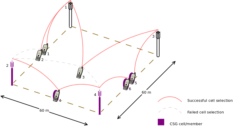
Sample result of cell selection test
The figure shows that CSG members may attach to either CSG or non-CSG cells, and simply choose the stronger one. On the other hand, non-members can only attach to non-CSG cells, even when they are actually receiving stronger signal from a CSG cell.
For reference purpose, Table UE error rate in Initial Cell Selection test shows the error rate of each UE when receiving transmission from the control channel. Based on this information, the check point time for UE #3 is done at a later time than the others to compensate for its higher risk of failure.
| UE # | Error rate |
|---|---|
| 1 | 0.00% |
| 2 | 1.44% |
| 3 | 12.39% |
| 4 | 0.33% |
| 5 | 0.00% |
| 6 | 0.00% |
The test uses the default Friis path loss model and without any channel fading model.
GTP-U protocol
The unit test suite epc-gtpu checks that the encoding and decoding of the GTP-U
header is done correctly. The test fills in a header with a set of
known values, adds the header to a packet, and then removes the header
from the packet. The test fails if, upon removing, any of the fields
in the GTP-U header is not decoded correctly. This is detected by
comparing the decoded value from the known value.
S1-U interface
Two test suites (epc-s1u-uplink and epc-s1u-downlink) make
sure that the S1-U interface implementation works correctly in
isolation. This is achieved by creating a set of simulation scenarios
where the EPC model alone is used, without the LTE model (i.e.,
without the LTE radio protocol stack, which is replaced by simple CSMA
devices). This checks that the
interoperation between multiple EpcEnbApplication instances in
multiple eNBs and the EpcSgwPgwApplication instance in the SGW/PGW
node works correctly in a variety of scenarios, with varying numbers
of end users (nodes with a CSMA device installed), eNBs, and different
traffic patterns (packet sizes and number of total packets).
Each test case works by injecting the chosen traffic pattern in the
network (at the considered UE or at the remote host for in the uplink or the
downlink test suite respectively) and checking that at the receiver
(the remote host or each considered UE, respectively) that exactly the same
traffic patterns is received. If any mismatch in the transmitted and
received traffic pattern is detected for any UE, the test fails.
TFT classifier
The test suite epc-tft-classifier checks in isolation that the
behavior of the EpcTftClassifier class is correct. This is performed
by creating different classifier instances where different TFT
instances are activated, and testing for each classifier that an
heterogeneous set of packets (including IP and TCP/UDP headers) is
classified correctly. Several test cases are provided that check the
different matching aspects of a TFT (e.g. local/remote IP address, local/remote port) both for uplink and
downlink traffic. Each test case corresponds to a specific packet and
a specific classifier instance with a given set of TFTs. The test case
passes if the bearer identifier returned by the classifier exactly
matches with the one that is expected for the considered packet.
End-to-end LTE-EPC data plane functionality
The test suite lte-epc-e2e-data ensures the correct end-to-end
functionality of the LTE-EPC data plane. For each test case in this
suite, a complete LTE-EPC simulation
scenario is created with the following characteristics:
- a given number of eNBs
- for each eNB, a given number of UEs
- for each UE, a given number of active EPS bearers
- for each active EPS bearer, a given traffic pattern (number of UDP packets to be transmitted and packet size)
Each test is executed by transmitting the given traffic pattern both in the uplink and in the downlink, at subsequent time intervals. The test passes if all the following conditions are satisfied:
- for each active EPS bearer, the transmitted and received traffic pattern (respectively at the UE and the remote host for uplink, and vice versa for downlink) is exactly the same
- for each active EPS bearer and each direction (uplink or downlink), exactly the expected number of packet flows over the corresponding RadioBearer instance
X2 handover
The test suite lte-x2-handover checks the correct functionality of the X2 handover procedure. The scenario being tested is a topology with two eNBs connected by an X2 interface. Each test case is a particular instance of this scenario defined by the following parameters:
- the number of UEs that are initially attached to the first eNB
- the number of EPS bearers activated for each UE
- a list of handover events to be triggered, where each event is defined by: + the start time of the handover trigger + the index of the UE doing the handover + the index of the source eNB + the index of the target eNB
- a boolean flag indicating whether the target eNB admits the handover or not
- a boolean flag indicating whether the ideal RRC protocol is to be used instead of the real RRC protocol
- the type of scheduler to be used (RR or PF)
Each test case passes if the following conditions are true:
- at time 0.06s, the test CheckConnected verifies that each UE is connected to the first eNB
- for each event in the handover list:
- at the indicated event start time, the indicated UE is connected to the indicated source eNB
- 0.1s after the start time, the indicated UE is connected to the indicated target eNB
- 0.6s after the start time, for each active EPS bearer, the uplink and downlink sink applications of the indicated UE have achieved a number of bytes which is at least half the number of bytes transmitted by the corresponding source applications
The condition “UE is connected to eNB” is evaluated positively if and only if all the following conditions are met:
- the eNB has the context of the UE (identified by the RNTI value retrieved from the UE RRC)
- the RRC state of the UE at the eNB is CONNECTED_NORMALLY
- the RRC state at the UE is CONNECTED_NORMALLY
- the UE is configured with the CellId, DlBandwidth, UlBandwidth, DlEarfcn and UlEarfcn of the eNB
- the IMSI of the UE stored at the eNB is correct
- the number of active Data Radio Bearers is the expected one, both at the eNB and at the UE
- for each Data Radio Bearer, the following identifiers match between the UE and the eNB: EPS bearer id, DRB id, LCID
Automatic X2 handover
The test suite lte-x2-handover-measures checks the correct functionality of the handover
algorithm. The scenario being tested is a topology with two, three or four eNBs connected by
an X2 interface. The eNBs are located in a straight line in the X-axes. A UE moves along the
X-axes going from the neighborhood of one eNB to the next eNB. Each test case is a particular
instance of this scenario defined by the following parameters:
- the number of eNBs in the X-axes
- the number of UEs
- the number of EPS bearers activated for the UE
- a list of check point events to be triggered, where each event is defined by: + the time of the first check point event + the time of the last check point event + interval time between two check point events + the index of the UE doing the handover + the index of the eNB where the UE must be connected
- a boolean flag indicating whether UDP traffic is to be used instead of TCP traffic
- the type of scheduler to be used
- the type of handover algorithm to be used
- a boolean flag indicating whether handover is admitted by default
- a boolean flag indicating whether the ideal RRC protocol is to be used instead of the real RRC protocol
The test suite consists of many test cases. In fact, it has been one of the most time-consuming test suite in ns-3. The test cases run with some combination of the following variable parameters:
- number of eNBs: 2, 3, 4;
- number of EPS bearers: 0, 1, 2;
- RRC: ideal, real (see RRC protocol models);
- MAC scheduler: round robin, proportional fair (see The FemtoForum MAC Scheduler Interface); and
- handover algorithm: A2-A4-RSRQ, strongest cell (see Handover algorithm).
Each test case passes if the following conditions are true:
- at time 0.08s, the test CheckConnected verifies that each UE is connected to the first eNB
- for each event in the check point list:
- at the indicated check point time, the indicated UE is connected to the indicated eNB
- 0.5s after the check point, for each active EPS bearer, the uplink and downlink sink applications of the UE have achieved a number of bytes which is at least half the number of bytes transmitted by the corresponding source applications
The condition “UE is connected to eNB” is evaluated positively if and only if all the following conditions are met:
- the eNB has the context of the UE (identified by the RNTI value retrieved from the UE RRC)
- the RRC state of the UE at the eNB is CONNECTED_NORMALLY
- the RRC state at the UE is CONNECTED_NORMALLY
- the UE is configured with the CellId, DlBandwidth, UlBandwidth, DlEarfcn and UlEarfcn of the eNB
- the IMSI of the UE stored at the eNB is correct
- the number of active Data Radio Bearers is the expected one, both at the eNB and at the UE
- for each Data Radio Bearer, the following identifiers match between the UE and the eNB: EPS bearer id, DRB id, LCID
Handover delays
Handover procedure consists of several message exchanges between UE, source
eNodeB, and target eNodeB over both RRC protocol and X2 interface. Test suite
lte-handover-delay verifies that this procedure consistently spends the
same amount of time.
The test suite will run several handover test cases. Each test case is an individual simulation featuring a handover at a specified time in simulation. For example, the handover in the first test case is invoked at time +0.100s, while in the second test case it is at +0.101s. There are 10 test cases, each testing a different subframe in LTE. Thus the last test case has the handover at +0.109s.
The simulation scenario in the test cases is as follow:
- EPC is enabled
- 2 eNodeBs with circular (isotropic) antenna, separated by 1000 meters
- 1 static UE positioned exactly in the center between the eNodeBs
- no application installed
- no channel fading
- default path loss model (Friis)
- 0.300s simulation duration
The test case runs as follow. At the beginning of the simulation, the UE is attached to the first eNodeB. Then at the time specified by the test case input argument, a handover request will be explicitly issued to the second eNodeB. The test case will then record the starting time, wait until the handover is completed, and then record the completion time. If the difference between the completion time and starting time is less than a predefined threshold, then the test passes.
A typical handover in the current ns-3 implementation takes 4.2141 ms when using Ideal RRC protocol model, and 19.9283 ms when using Real RRC protocol model. Accordingly, the test cases use 5 ms and 20 ms as the maximum threshold values. The test suite runs 10 test cases with Ideal RRC protocol model and 10 test cases with Real RRC protocol model. More information regarding these models can be found in Section RRC protocol models.
The motivation behind using subframes as the main test parameters is the fact that subframe index is one of the factors for calculating RA-RNTI, which is used by Random Access during the handover procedure. The test cases verify this computation, utilizing the fact that the handover will be delayed when this computation is broken. In the default simulation configuration, the handover delay observed because of a broken RA-RNTI computation is typically 6 ms.
Selection of target cell in handover algorithm
eNodeB may utilize Handover algorithm to automatically create handover decisions during simulation. The decision includes the UE which should do the handover and the target cell where the UE should perform handover to.
The test suite lte-handover-target verifies that the handover algorithm is
making the right decision, in particular, in choosing the right target cell. It
consists of several short test cases for different network topology (2×2 grid
and 3×2 grid) and types of handover algorithm (the A2-A4-RSRQ handover algorithm
and the strongest cell handover algorithm).
Each test case is a simulation of a micro-cell environment with the following parameter:
- EPC is enabled
- several circular (isotropic antenna) micro-cell eNodeBs in a rectangular grid layout, with 130 m distance between each adjacent point
- 1 static UE, positioned close to and attached to the source cell
- no control channel error model
- no application installed
- no channel fading
- default path loss model (Friis)
- 1s simulation duration
To trigger a handover, the test case “shutdowns” the source cell at +0.5s simulation time. Figure lte-handover-target test scenario in a 2×2 grid below illustrates the process. This is done by setting the source cell’s Tx power to a very low value. As a result, the handover algorithm notices that the UE deserves a handover and several neighboring cells become candidates of target cell at the same time.
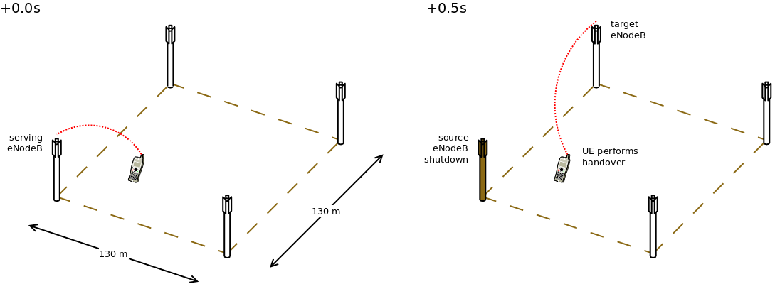
lte-handover-target test scenario in a 2×2 grid
The test case then verifies that the handover algorithm, when faced with more than one options of target cells, is able to choose the right one.
Downlink Power Control
The test suite lte-downlink-power-control checks correctness of Downlink
Power Control in three different ways:
- LteDownlinkPowerControlSpectrumValue test case check if
LteSpectrumValueHelper::CreateTxPowerSpectralDensityis creating correct spectrum value for PSD for downlink transmission. The test vector contain EARFCN, system bandwidth, TX power, TX power for each RB, active RBs, and expected TxPSD. The test passes if TxPDS generated byLteSpectrumValueHelper::CreateTxPowerSpectralDensityis equal to expected TxPSD.- LteDownlinkPowerControlTestCase test case check if TX power difference between data and control channel is equal to configured PdschConfigDedicated::P_A value. TX power of control channel is measured by
LteTestSinrChunkProcessoradded toRsPowerChunkProcessorlist in UE DownlinkSpectrumPhy. Tx power of data channel is measured in similar way, but it had to be implemented. NowLteTestSinrChunkProcessoris added toDataPowerChunkProcessorlist in UE DownlinkSpectrumPhy. Test vector contain a set of all available P_A values. Test pass if power difference equals P_A value.- LteDownlinkPowerControlRrcConnectionReconfiguration test case check if RrcConnectionReconfiguration is performed correctly. When FR entity gets UE measurements, it immediately calls function to change P_A value for this UE and also triggers callback connected with this event. Then, test check if UE gets RrcConnectionReconfiguration message (it trigger callback). Finally, it checks if eNB receive RrcConnectionReconfigurationCompleted message, what also trigger callback. The test passes if all event have occurred. The test is performed two times, with IdealRrcProtocol and with RealRrcProtocol.
Uplink Power Control Tests
UE uses Uplink Power Control to automatically change Tx Power level for Uplink Physical Channels. Tx Power is computed based on path-loss, number of RB used for transmission, some configurable parameters and TPC command from eNB.
The test suite lte-uplink-power-control verifies if Tx Power is computed correctly.
There are three different test cases:
- LteUplinkOpenLoopPowerControlTestCase test case checks Uplink Power Control functionality in Open Loop mechanism. UE is attached to eNB and is transmitting data in Downlink and Uplink. Uplink Power Control with Open Loop mechanism is enabled and UE changes position each 100 ms. In each position Uplink Power Control entity is calculating new Tx Power level for all uplink channels. These values are traced and test passes if Uplink Tx Power for PUSCH, PUCCH and SRS in each UE position are equal to expected values.
- LteUplinkClosedLoopPowerControlAbsoluteModeTestCase test case checks Uplink Power Control functionality with Closed Loop mechanism and Absolute Mode enabled. UE is attached to eNB and is transmitting data in Downlink and Uplink. Uplink Power Control with Closed Loop mechanism and Absolute Mode is enabled. UE is located 100 m from eNB and is not changing its position. LteFfrSimple algorithm is used on eNB side to set TPC values in DL-DCI messages. TPC configuration in eNB is changed every 100 ms, so every 100 ms Uplink Power Control entity in UE should calculate different Tx Power level for all uplink channels. These values are traced and test passes if Uplink Tx Power for PUSCH, PUCCH and SRS computed with all TCP values are equal to expected values.
- LteUplinkClosedLoopPowerControlAccumulatedModeTestCase test case checks Closed Loop Uplink Power Control functionality with Closed Loop mechanism and Accumulative Mode enabled. UE is attached to eNB and is transmitting data in Downlink and Uplink. Uplink Power Control with Closed Loop mechanism and Accumulative Mode is enabled. UE is located 100 m from eNB and is not changing its position. As in above test case, LteFfrSimple algorithm is used on eNB side to set TPC values in DL-DCI messages, but in this case TPC command are set in DL-DCI only configured number of times, and after that TPC is set to be 1, what is mapped to value of 0 in Accumulative Mode (TS36.213 Table 5.1.1.1-2). TPC configuration in eNB is changed every 100 ms. UE is accumulating these values and calculates Tx Power levels for all uplink channels based on accumulated value. If computed Tx Power level is lower than minimal UE Tx Power, UE should transmit with its minimal Tx Power. If computed Tx Power level is higher than maximal UE Tx Power, UE should transmit with its maximal Tx Power. Tx Power levels for PUSCH, PUCCH and SRS are traced and test passes if they are equal to expected values.
Frequency Reuse Algorithms
The test suite lte-frequency-reuse contain two types of test cases.
First type of test cases check if RBGs are used correctly according to FR algorithm
policy. We are testing if scheduler use only RBGs allowed by FR configuration. To
check which RBGs are used LteSimpleSpectrumPhy is attached to Downlink Channel.
It notifies when data downlink channel transmission has occurred and pass signal
TxPsd spectrum value to check which RBs were used for transmission. The test vector
comprise a set of configuration for Hard and Strict FR algorithms (there is no point
to check other FR algorithms in this way because they use entire cell bandwidth).
Test passes if none of not allowed RBGs are used.
Second type of test cases check if UE is served within proper sub-band and with proper
transmission power. In this test scenario, there are two eNBs.There are also two UEs
and each eNB is serving one. One uses Frequency Reuse algorithm and second one does not.
Second eNB is responsible for generating interferences in whole system bandwidth.
UE served by first eNB is changing position each few second (rather slow because time is
needed to report new UE Measurements). To check which RBGs are used for this UE
LteSimpleSpectrumPhy is attached to Downlink Channel. It notifies when data
downlink channel transmission in cell 1 has occurred and pass signal TxPsd spectrum value
to check which RBs were used for transmission and their power level.
The same approach is applied in Uplink direction and second LteSimpleSpectrumPhy
is attached to Uplink Channel. Test passes if UE served by eNB with FR algorithm
is served in DL and UL with expected RBs and with expected power level.
Test vector comprise a configuration for Strict FR, Soft FR, Soft FFR, Enhanced FFR.
Each FR algorithm is tested with all schedulers, which support FR (i.e. PF, PSS, CQA,
TD-TBFQ, FD-TBFQ). (Hard FR do not use UE measurements, so there is no point to perform
this type of test for Hard FR).
Test case for Distributed FFR algorithm is quite similar to above one, but since eNBs need
to exchange some information, scenario with EPC enabled and X2 interfaces is considered.
Moreover, both eNB are using Distributed FFR algorithm. There are 2 UE in first cell,
and 1 in second cell. Position of each UE is changed (rather slow because time is
needed to report new UE Measurements), to obtain different result from calculation in
Distributed FFR algorithm entities. To check which RBGs are used for UE transmission
LteSimpleSpectrumPhy is attached to Downlink Channel. It notifies when data
downlink channel transmission has occurred and pass signal TxPsd spectrum value
to check which RBs were used for transmission and their power level.
The same approach is applied in Uplink direction and second LteSimpleSpectrumPhy
is attached to Uplink Channel.
Test passes if UE served by eNB in cell 2, is served in DL and UL with expected RBs
and with expected power level. Test vector comprise a configuration for Distributed FFR.
Test is performed with all schedulers, which support FR (i.e. PF, PSS, CQA,
TD-TBFQ, FD-TBFQ).
Inter-cell Interference with FR algorithms Tests
The test suite lte-interference-fr is very similar to lte-interference.
Topology (Figure Topology for the inter-cell interference test) is the same and test checks
interference level. The difference is that, in this test case Frequency Reuse algorithms
are enabled and we are checking interference level on different RBGs (not only on one).
For example, when we install Hard FR algorithm in eNbs, and first half of system bandwidth
is assigned to one eNb, and second half to second eNb, interference level should be much
lower compared to legacy scenario. The test vector comprise a set of configuration for
all available Frequency Reuse Algorithms. Test passes if calculated SINR on specific
RBs is equal to these obtained by Octave script.
Carrier aggregation test
The test suite lte-carrier-aggregation is a system test program that creates different test
cases with a single eNB and several UEs, all having the same radio bearer specification. Different
test cases are implemented by using different SINR values and different numbers of UEs. eNBs and UEs
are configured to use the secondary carrier and the component carrier manager is configured to
split the data uniformly between primary and secondary carrier. The test consists of checking that
the throughput obtained over the different carriers are equal considering a given tolerance. For more
details about this test, see the section Carrier aggregation usage example.
Carrier aggregation test for eNB and UE configuration
The test suite carrier-aggregation-config-test is a system test program, which verifies the
following two cases:
- When carrier aggregation is enabled and UE carriers configuration is different than the default configuration done in LteHelper, we check that the UE(s) is configured properly once it receives RRC Connection Reconfiguration message from eNB.
- A user can configure 2 or more eNBs and UEs with different configuration parameters, i.e., each eNB and UE can have different EARFCN and Bandwidths and a UE connects to an eNB with similar DL EARFCN. In this test, we check with CA enabled but the end results will be the same if carrier aggregation is not enabled and we have more than one eNBs and UEs with different configurations.
Since, we do not need EPC to test the configuration, this test only simulates the LTE radio access with RLC SM.
There are two test cases, Test 1 tests that the UE is configured properly after receiving RRC Connection Reconfiguration
message from the eNB, which will overwrite UE default configuration done in LteHelper for the sake of
creating PHY and MAC instances equal to the number of component carriers. Test 2 tests that every eNB or UE in a
simulation scenario can be configured with different EARFCNs and Bandwidths. For both test cases, it also counts
the number of times the hooked trace source SCarrierConfigured get triggered. As, it reflects how many UEs
got attached to their respective eNB. If the count is not equal to the number of UEs in the scenario, the test fails,
which could be the result of improper UE configuration.
Radio link failure Test
The test suite lte-radio-link-failure is a system test, which tests the
radio link failure functionality using Ideal and Real RRC protocols.
In particular, it tests the following to verify the Radio link
Failure (RLF) implementation.
- The state and the configuration of the UE while it is connected to the eNB.
- The state of the UE while T310 timer is running at the UE.
- The number of out-of-sync and in-synch indications received.
- The state of the UE before the simulation end.
- The UE context existence at the eNB before the simulation end.
This test simulates only one static UE with EPC performing downlink and uplink communication in the following two scenarios:
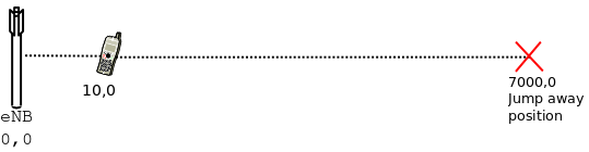
RLF scenario with one eNB
In this scenario, the UE is initially placed near to the eNB, and on the following instances above conditions are verified against the expected outcome.
At 0.3 sec: It verifies that the UE is well connected, i.e., it is in “CONNECTED_NORMALLY” state, and is attached to the eNB with cell id 1. It also checks for the match between the configuration of the UE and the UE context at the eNB, e.g., IMSI, bandwidth, D/UL EARFCN, number of bearers and the bearer IDs. The miss match would result in the test suite failure.
At 0.4 sec: The UE jumps far away from the eNB, which causes the DL SINR at the UE to fall below -5 dB. In result, the UE PHY after monitoring the SINR for 20 consecutive frames will send a notification to the UE RRC. In this test, the N310 counter is set to 1; thus, the UE RRC will start the T310 (set to 1 sec) timer upon the first notification from the PHY layer.
At 1 sec: At this stage, it is expected that the T310 timer is still running, and the UE is connected to the eNB.
Upon RLF: It is expected that the UE RRC will start the T310 timer upon reaching the configured, i.e., N310 = 1 number of notification from the eNB. The RRC will receive no in-sync indication since the UE stays at far away position.
Before the end of simulation: The expected behavior is that the UE state will be in “IDLE_CELL_SEARCH” since there is no eNB available where it has jumped. Moreover, the deletion of the UE context from the eNB is also verified.
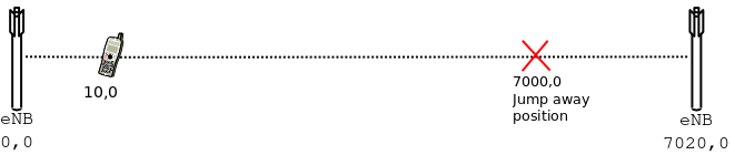
RLF scenario with two eNBs
In this scenario, the only difference is the addition of a second eNB near the position where the UE jumps away. Therefore, except the outcome before the end of the simulation, all the outcomes are similar to that we expected in the first scenario.
Before the end of simulation: It is expected that the UE after the RLF will connect to the second eNB, i.e., it will be in “CONNECTED_NORMALLY” state, and its context exists in the second eNB.
Profiling Documentation
Overview and objectives
The main objective of the profiling carried out is to assess the simulator performance on a broad set of scenarios. This evaluation provides reference values for simulation running times and memory consumption figures. It also helps to identify potential performance improvements and to check for scalability problems when increasing the number of eNodeB and UEs attached to those.
In the following sections, a detailed description of the general profiling framework employed to perform the study is introduced. It also includes details on the main performed tests and its results evaluation.
Framework description
Simulation scripts
The simulation script used for all the E-UTRAN results showed in this documentation is located at src/lte/examples/lena-profiling.cc. It uses the complete PHY and MAC UE/eNodeB implementation with a simplified RLC implementation on top. This script generates a squared grid topology, placing a eNodeB at the centre of each square. UEs attached to this node are scattered randomly across the square (using a random uniform distribution along X and Y axis). If BuildingPropagationModel is used, the squares are replaced by rooms. To generate the UL and DL traffic, the RLC implementation always report data to be transferred.
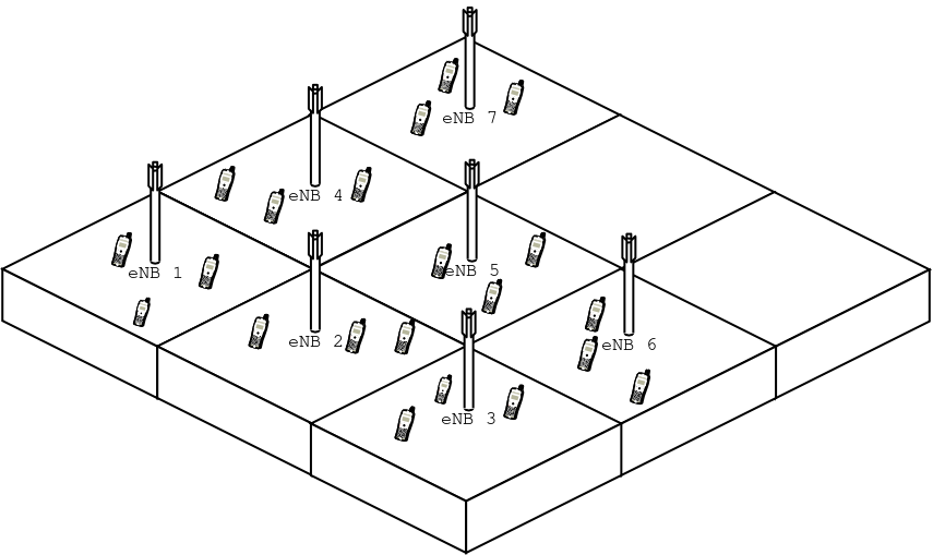
E-UTRAN
For the EPC results, the script is src/lte/examples/lena-simple-epc.cc. It uses a complete E-UTRAN implementation (PHY+MAC+RLC/UM+PDCP) and the most relevant EPC user plane entities the PGW and SGW, including GTP-U tunneling. This script generates a given number of eNodeBs, distributed across a line and attaches a single UE to every eNodeB. It also creates an EPC network and an external host connected to it through the Internet. Each UE sends and receives data to and from the remote host. In addition, each UE is also sending data to the UE camped in the adjacent eNodeB.
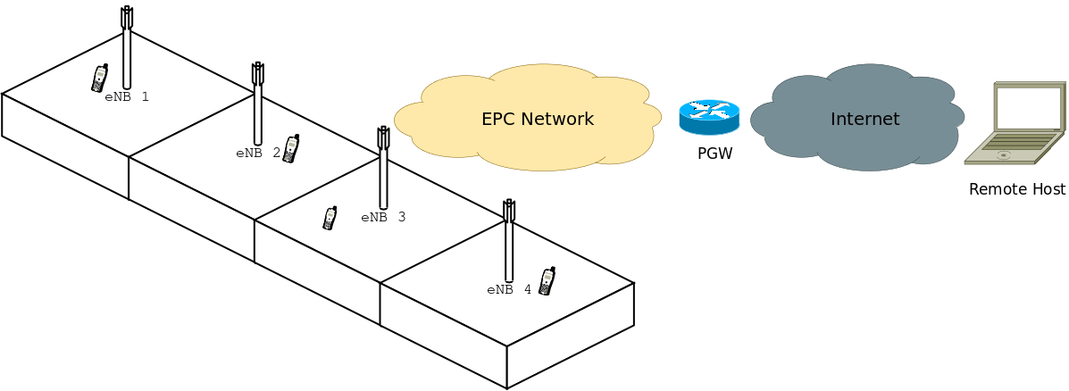
Propagation Model
RLC and MAC traces are enabled for all UEs and all eNodeBs and those traces are written to disk directly. The MAC scheduler used is round robin.
Simulation input parameters
The lena-profiling simulation script accepts the following input parameters:
simTime: time to simulate (in seconds)nUe: number of UEs attached to each eNodeBnEnb: number of eNodeB composing the grid per floornFloors: number of floors, 0 for Friis propagation model (no walls), 1 or greater for Building propagation model generating a nFloors-storey building.traceDirectory: destination directory where simulation traces will be stored
The lena-simple-epc script accepts those other parameters:
simTime: time to simulate (in seconds)numberOfNodes: number of eNodeB + UE pairs created
Time measurement
Running time is measured using default Linux shell command time. This command counts how much user time the execution of a program takes.
Perl script
To simplify the process of running the profiling script for a wide range of values and collecting its timing data, a simple Perl script to automate the complete process is provided. It is placed in src/lte/test/lte-test-run-time.pl for lena-profiling and in src/lte/epc-test-run-time.pl for lena-simple-epc. It simply runs a batch of simulations with a range of parameters and stores the timing results in a CSV file called lteTimes.csv and epcTimes.csv respectively. The range of values each parameter sweeps can be modified editing the corresponding script.
Requirements
- The following Perl modules are required to use the provided script, all of them available from CPAN:
- IO::CaptureOutput
- Statistics::Descriptive
For installing the modules, simply use the following command:
perl -MCPAN -e 'install moduleName'
Plotting results
To plot the results obtained from running the Perl scripts, two gnuplot scripts are provided, in src/lte/test/lte-test-run-plot and src/lte/test/epc-test-run-plot. Most of the plots available in this documentation can be reproduced with those, typing the commands gnuplot < src/lte/test/lte-test-run-plot and gnuplot < src/lte/test/epc-test-run-plot.
Reference software and equipment
All timing tests had been run in a Intel Pentium IV 3.00 GHz machine with 512 Mb of RAM memory running Fedora Core 10 with a 2.6.27.41-170.2.117 kernel, storing the traces directly to the hard disk.
Also, as a reference configuration, the build has been configured static and optimized. The exact waf command issued is:
CXXFLAGS="-O3 -w" ./waf -d optimized configure --enable-static --enable-examples --enable-modules=lte
Results
E-UTRAN
The following results and figures had been obtained with LENA changeset 2c5b0d697717.
Running time
This scenario, evaluates the running time for a fixed simulation time (10s) and Friis propagation mode increasing the number of UEs attached to each eNodeB and the number of planted eNodeBs in the scenario.
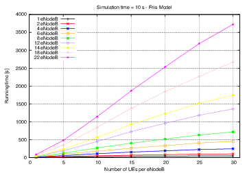
Running time
The figure shows the expected behaviour, since it increases linearly respect the number of UEs per eNodeB and quadratically respect the total number of eNodeBs.
Propagation model
The objective of this scenario is to evaluate the impact of the propagation model complexity in the overall run time figures. Therefore, the same scenario is simulated twice: once using the more simple Friis model, once with the more complex Building model. The rest of the parameters (e.g. number of eNodeB and of UE attached per eNodeB) were maintained. The timing results for both models are compared in the following figure.
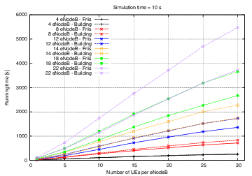
Propagation Model
In this situation, results are also coherent with what is expected. The more complex the model, the higher the running time. Moreover, as the number of computed path losses increases (i.e. more UEs per eNodeB or more eNodeBs) the extra complexity of the propagation model drives the running time figures further apart.
Simulation time
In this scenario, for a fixed set of UEs per eNodeB, different simulation times had been run. As the simulation time increases, running time should also increase linearly, i.e. for a given scenario, simulate four seconds should take twice times what it takes to simulate two seconds. The slope of this line is a function of the complexity of the scenario: the more eNodeB / UEs placed, the higher the slope of the line.
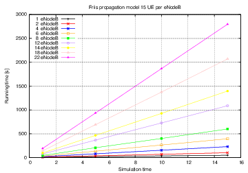
Simulation time
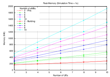
EPC
The following results and figures had been obtained with LENA changeset e8b3ccdf6673. The rationale behind the two scenarios profiled on this section is the same than for the E-UTRA part.
Running time
Running time evolution is quadratic since we increase at the same time the number of eNodeB and the number of UEs.
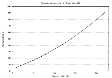
Running time
To estimate the additional complexity of the upper LTE Radio Protocol Stack model and the EPC model, we compare two scenarios using the simplified E-UTRAN version (using only PHY, MAC and the simplified RLC/SM, with no EPC and no ns-3 applications) against the complete E-UTRAN + EPC (with UM RLC, PDCP, end-to-end IP networking and regular ns-3 applications). Both configuration have been tested with the same number of UEs per eNodeB, the same number of eNodeBs, and approximately the same volume of transmitted data (an exact match was not possible due to the different ways in which packets are generated in the two configurations).
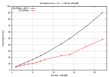
EPC E-UTRAN running time
From the figure, it is evident that the additional complexity of using the upper LTE stack plus the EPC model translates approximately into a doubling of the execution time of the simulations. We believe that, considered all the new features that have been added, this figure is acceptable.
Simulation time
Finally, again the linearity of the running time as the simulation time increases gets validated through a set of experiments, as the following figure shows.
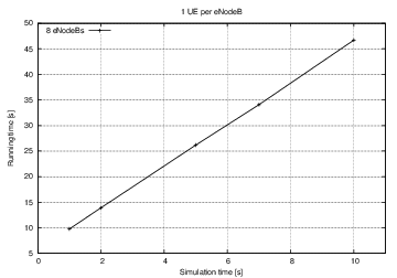
Simulation time
References
| [TS25814] | 3GPP TS 25.814 “Physical layer aspect for evolved Universal Terrestrial Radio Access” |
| [TS29274] | 3GPP TS 29.274 “GPRS Tunnelling Protocol for Control plane (GTPv2-C)” |
| [TS36101] | 3GPP TS 36.101 “E-UTRA User Equipment (UE) radio transmission and reception” |
| [TS36104] | 3GPP TS 36.104 “E-UTRA Base Station (BS) radio transmission and reception” |
| [TS36133] | 3GPP TS 36.133 “E-UTRA Requirements for support of radio resource management” |
| [TS36211] | 3GPP TS 36.211 “E-UTRA Physical Channels and Modulation” |
| [TS36212] | 3GPP TS 36.212 “E-UTRA Multiplexing and channel coding” |
| [TS36213] | 3GPP TS 36.213 “E-UTRA Physical layer procedures” |
| [TS36214] | 3GPP TS 36.214 “E-UTRA Physical layer – Measurements” |
| [TS36300] | 3GPP TS 36.300 “E-UTRA and E-UTRAN; Overall description; Stage 2” |
| [TS36304] | 3GPP TS 36.304 “E-UTRA User Equipment (UE) procedures in idle mode” |
| [TS36321] | 3GPP TS 36.321 “E-UTRA Medium Access Control (MAC) protocol specification” |
| [TS36322] | 3GPP TS 36.322 “E-UTRA Radio Link Control (RLC) protocol specification” |
| [TS36323] | 3GPP TS 36.323 “E-UTRA Packet Data Convergence Protocol (PDCP) specification” |
| [TS36331] | 3GPP TS 36.331 “E-UTRA Radio Resource Control (RRC) protocol specification” |
| [TS36413] | 3GPP TS 36.413 “E-UTRAN S1 application protocol (S1AP)” |
| [TS36420] | 3GPP TS 36.420 “E-UTRAN X2 general aspects and principles” |
| [TS36423] | 3GPP TS 36.423 “E-UTRAN X2 application protocol (X2AP)” |
| [TR36814] | 3GPP TR 36.814 “E-UTRA Further advancements for E-UTRA physical layer aspects” |
| [R1-081483] | 3GPP R1-081483 “Conveying MCS and TB size via PDCCH” |
| [R4-092042] | 3GPP R4-092042 “Simulation assumptions and parameters for FDD HeNB RF requirements” |
| [FFAPI] | FemtoForum “LTE MAC Scheduler Interface Specification v1.11” |
| [ns3tutorial] | “The ns-3 Tutorial” |
| [ns3manual] | “The ns-3 Manual” |
| [Sesia2009] | S. Sesia, I. Toufik and M. Baker, “LTE - The UMTS Long Term Evolution - from theory to practice”, Wiley, 2009 |
| [Baldo2009] | N. Baldo and M. Miozzo, “Spectrum-aware Channel and PHY layer modeling for ns3”, Proceedings of ICST NSTools 2009, Pisa, Italy |
| [Piro2010] | Giuseppe Piro, Luigi Alfredo Grieco, Gennaro Boggia, and Pietro Camarda, “A Two-level Scheduling Algorithm for QoS Support in the Downlink of LTE Cellular Networks”, Proc. of European Wireless, EW2010, Lucca, Italy, Apr., 2010 |
| [Holtzman2000] | J.M. Holtzman, “CDMA forward link waterfilling power control”, in Proc. of IEEE VTC Spring, 2000. |
| [Piro2011] | G. Piro, N. Baldo. M. Miozzo, “An LTE module for the ns-3 network simulator”, in Proc. of Wns3 2011 (in conjunction with SimuTOOLS 2011), March 2011, Barcelona (Spain) |
| [Seo2004] | H. Seo, B. G. Lee. “A proportional-fair power allocation scheme for fair and efficient multiuser OFDM systems”, in Proc. of IEEE GLOBECOM, December 2004. Dallas (USA) |
| [Ofcom2600MHz] | Ofcom, “Consultation on assessment of future mobile competition and proposals for the award of 800 MHz and 2.6 GHz spectrum and related issues”, March 2011 |
| [RealWireless] | RealWireless, “Low-power shared access to spectrum for mobile broadband”, Final Report, Ofcom Project MC/073, 18th March 2011 |
| [PaduaPEM] | “Ns-developers - LTE error model contribution” |
| [ViennaLteSim] | “The Vienna LTE Simulators” |
| [LozanoCost] | Joan Olmos, Silvia Ruiz, Mario García-Lozano and David Martín-Sacristán, “Link Abstraction Models Based on Mutual Information for LTE Downlink”, COST 2100 TD(10)11052 Report |
| [wimaxEmd] | WiMAX Forum White Paper, “WiMAX System Evaluation Methodology”, July 2008. |
| [mathworks] | Matlab R2011b Documentation Communications System Toolbox, “Methodology for Simulating Multipath Fading Channels” |
| [CatreuxMIMO] | S. Catreux, L.J. Greenstein, V. Erceg, “Some results and insights on the performance gains of MIMO systems,” Selected Areas in Communications, IEEE Journal on , vol.21, no.5, pp. 839- 847, June 2003 |
| [Ikuno2010] | J.C. Ikuno, M. Wrulich, M. Rupp, “System Level Simulation of LTE Networks,” Vehicular Technology Conference (VTC 2010-Spring), 2010 IEEE 71st , vol., no., pp.1-5, 16-19 May 2010 |
| [Milos2012] | J. Milos, “Performance Analysis Of PCFICH LTE Control Channel”, Proceedings of the 19th Conference STUDENT EEICT 2012, Brno, CZ, 2012. |
| [FujitsuWhitePaper] | “Enhancing LTE Cell-Edge Performance via PDCCH ICIC”. |
| [Bharucha2011] | Z. Bharucha, G. Auer, T. Abe, N. Miki, “Femto-to-Macro Control Channel Interference Mitigation via Cell ID Manipulation in LTE,” Vehicular Technology Conference (VTC Fall), 2011 IEEE , vol., no., pp.1-6, 5-8 Sept. 2011 |
| [R4-081920] | 3GPP R4-081920 “LTE PDCCH/PCFICH Demodulation Performance Results with Implementation Margin” |
| [FCapo2012] | F.Capozzi, G.Piro, L.A. Grieco, G.Boggia, P.Camarda, “Downlink Packet Scheduling in LTE Cellular Networks: Key Design Issues and a Survey”, IEEE Comm. Surveys and Tutorials, vol.2012, no.99, pp.1-23, Jun. 2012 |
| [FABokhari2009] | F.A. Bokhari, H. Yanikomeroglu, W.K. Wong, M. Rahman, “Cross-Layer Resource Scheduling for Video Traffic in the Downlink of OFDMA-Based Wireless 4G Networks”, EURASIP J. Wirel. Commun. Netw., vol.2009, no.3, pp. 1-10, Jan. 2009. |
| [WKWong2004] | W.K. Wong, H.Y. Tang, V.C.M, Leung, “Token bank fair queuing: a new scheduling algorithm for wireless multimedia services”, Int. J. Commun. Syst., vol.17, no.6, pp.591-614, Aug.2004. |
| [GMonghal2008] | G. Mongha, K.I. Pedersen, I.Z. Kovacs, P.E. Mogensen, “QoS Oriented Time and Frequency Domain Packet Schedulers for The UTRAN Long Term Evolution”, In Proc. IEEE VTC, 2008. |
| [Dimou2009] | K. Dimou, M. Wang, Y. Yang, M. Kazmi, A. Larmo, J. Pettersson, W. Muller, Y. Timner, “Handover within 3GPP LTE: Design Principles and Performance”, Vehicular Technology Conference Fall (VTC 2009-Fall), 2009 IEEE 70th, pp.1-5, 20-23 Sept. 2009 |
| [Lee2010] | Y.J. Lee, B.J. Shin, J.C. Lim, D.H. Hong, “Effects of time-to-trigger parameter on handover performance in SON-based LTE systems”, Communications (APCC), 2010 16th Asia-Pacific Conference on, pp.492-496, Oct. 31 2010–Nov. 3 2010 |
| [Bbojovic2014] | B. Bojovic, N. Baldo, “A new Channel and QoS Aware Scheduler to enhance the capacity of Voice over LTE systems”, in Proceedings of 11th International Multi-Conference on Systems, Signals & Devices (SSD’14), Castelldefels, 11-14 February 2014, Castelldefels (Spain). |
| [Baldo2014] | N. Baldo, R. Martínez, P. Dini, R. Vilalta, M. Miozzo, R. Casellas, R. Muñoz, “A Testbed for Fixed Mobile Convergence Experimentation: ADRENALINE-LENA Integration”, in Proceedings of European Wireless 2014, 14-16 May 2014, Barcelona (Spain). |
| [ASHamza2013] | Abdelbaset S. Hamza, Shady S. Khalifa, Haitham S. Hamza, and Khaled Elsayed, “A Survey on Inter-Cell Interference Coordination Techniques in OFDMA-based Cellular Networks”, IEEE Communications Surveys & Tutorials, March 19, 2013 |
| [ZXie2009] | Zheng Xie, Bernhard Walke, “Enhanced Fractional Frequency Reuse to Increase Capacity of OFDMA Systems”, Proceedings of the 3rd international conference on New technologies, mobility and security, NTMS 2009 |
| [DKimura2012] |
|
Wi-Fi Mesh Module Documentation
Design Documentation
Overview
The ns-3 mesh module extends the ns-3 wifi module to provide mesh networking capabilities according to the IEEE 802.11s standard [ieee80211s].
The basic purpose of IEEE 802.11s is to define a mode of operation for Wi-Fi that permits frames to be forwarded over multiple radio hops transparent to higher layer protocols such as IP. To accomplish this, mesh-capable stations form a Mesh Basic Service Set (MBSS) by running a pair-wise peering protocol to establish forwarding associations, and by running a routing protocol to find paths through the network. A special gateway device called a mesh gate allows a MBSS to interconnect with a Distribution System (DS).
The basic enhancements defined by IEEE 802.11s include:
- discovery services
- peering management
- security
- beaconing and synchronization
- the Mesh Coordination Function (MCF)
- power management
- channel switching
- extended frame formats
- path selection and forwarding
- interworking (proxy mesh gateways)
- intra-mesh congestion control, and
- emergency service support.
The ns-3 models implement only a subset of the above service extensions, focusing mainly on those items related to peering and routing/forwarding of data frames through the mesh.
The Mesh NetDevice based on 802.11s D3.0 draft standard was added in ns-3.6 and includes the Mesh Peering Management Protocol and HWMP (routing) protocol implementations. An overview presentation by Kirill Andreev was published at the Workshop on ns-3 in 2009 [And09]. An overview paper is available at [And10].
As of ns-3.23 release, the model has been updated to the 802.11s-2012 standard [ieee80211s] with regard to packet formats, based on the contribution in [Hep15].
These changes include:
- Category codes and the categories compliant to IEEE-802.11-2012 Table 8-38—Category values.
- Information Elements (An adjustment of the element ID values was needed according to Table 8-54 of IEEE-802.11-2012).
- Mesh Peering Management element format changed according to IEEE-802.11-2012 Figure 8-370.
- Mesh Configuration element format changed according to IEEE-802.11-2012 Figure 8-363.
- PERR element format changed according to IEEE-802.11-2012 Figure 8-394.
With these changes the messages of the Peering Management Protocol and Hybrid Wireless Mesh Protocol will be transmitted compliant to IEEE802.11-2012 and the resulting pcap trace files can be analyzed by Wireshark.
The multi-interface mesh points are supported as an extension of IEEE draft version 3.0. Note that corresponding ns-3 mesh device helper creates a single interface station by default.
Overview of IEEE 802.11s
The implementation of the 802.11s extension consists of two main parts: the Peer Management Protocol (PMP) and Hybrid Wireless Mesh Protocol (HWMP).
The tasks of the peer management protocol are the following:
- opening links, detecting beacons, and starting peer link finite state machine, and
- closing peer links due to transmission failures or beacon loss.
If a peer link between the sender and receiver does not exist, a frame will be
dropped. So, the plug-in to the peer management protocol (PMP) is the first
in the list of ns3::MeshWifiInterfaceMacPlugins to be used.
Peer management protocol
The peer management protocol consists of three main parts:
- the protocol itself,
ns3::dot11s::PeerManagementProtocol, which keeps all active peer links on interfaces, handles all changes of their states and notifies the routing protocol about link failures. - the MAC plug-in,
ns3::dot11s::PeerManagementProtocolMac, which drops frames if there is no peer link, and peeks all needed information from management frames and information elements from beacons. - the peer link,
ns3::dot11s::PeerLink, which keeps finite state machine of each peer link, keeps beacon loss counter and counter of successive transmission failures.
The procedure of closing a peer link is not described in detail in the standard, so in the model the link may be closed by:
- beacon loss (see an appropriate attribute of ns3::dot11s::PeerLink class)
- transmission failure – when a predefined number of successive packets have failed to transmit, the link will be closed.
The peer management protocol is also responsible for beacon collision avoidance, because it keeps beacon timing elements from all neighbours. Note that the PeerManagementProtocol is not attached to the MeshPointDevice as a routing protocol, but the structure is similar: the upper tier of the protocol is
ns3::dot11s::PeerManagementProtocol and its plug-in is
ns3::dot11s::PeerManagementProtocolMac.
Hybrid Wireless Mesh Protocol
HWMP is implemented in both modes, reactive and proactive, although path maintenance is not implemented (so active routes may time out and need to be rebuilt, causing packet loss). Also the model implements an ability to transmit broadcast data and management frames as unicasts (see appropriate attributes). This feature is disabled at a station when the number of neighbors of the station is more than a threshold value.
Scope and Limitations
Supported features
- Peering Management Protocol (PMP), including link close heuristics and beacon collision avoidance.
- Hybrid Wireless Mesh Protocol (HWMP), including proactive and reactive modes, unicast/broadcast propagation of management traffic, multi-radio extensions.
- 802.11e compatible airtime link metric.
Verification
- Comes with the custom Wireshark dissector.
- Linux kernel mac80211 layer compatible message formats.
Unsupported features
- Mesh Coordinated Channel Access (MCCA).
- Internetworking: mesh access point and mesh portal.
- Security.
- Power save.
- Path maintenance (sending PREQ proactively before a path expires)
- Though multi-radio operation is supported, no channel assignment protocol is proposed for now. (Correct channel switching is not implemented)
Models yet to be created
- Mesh access point (QoS + non-QoS?)
- Mesh portal (QoS + non-QoS?)
Open issues
A bug exists in the Wi-Fi module that manifests itself as performance degradation in large mesh networks, due to incorrect duplicate frame detection for QoS data frames (bug 2326).
Mesh does not work for 802.11n/ac stations (bug 2276).
Energy module can not be used on mesh devices (bug 2265).
IE11S_MESH_PEERING_PROTOCOL_VERSION should be removed as per standard. Protocol ID should actually be part of the Mesh Peering Management IE (bug 2600).
Node packet processing times are not modeled; some evaluation of the impact of packet processing delays is discussed in [Hep16].
Testing Documentation
References
| [And09] | K. Andreev, Realization of IEEE802.11s draft standard in NS-3. |
| [And10] | K. Andreev and P. Boyko, IEEE 802.11s Mesh Networking NS-3 Model. |
| [Hep15] | C. Hepner and A. Witt and R. Muenzner, Validation of the ns-3 802.11s model and proposed changes compliant to IEEE 802.11-2012, Poster at 2015 Workshop on ns-3, May 2015. |
| [Hep16] | C. Hepner and S. Moll and R. Muenzner, Influence of Processing Delays on the VoIP Performance for IEEE 802.11s Multihop Wireless Mesh Networks: Comparison of ns-3 Network Simulations with Hardware Measurements, Proceedings of SIMUTOOLS 16, August, 2016. |
| [ieee80211s] | IEEE Standard for Information Technology, Telecommunications and information exchange between systems, Local and metropolitan area networks, Specific requirements, Part 11: Wireless LAN Medium Access Control (MAC) and Physical Layer (PHY) specifications, Amendment 10: Mesh Networking, 10 September 2011. |
MPI for Distributed Simulation
Parallel and distributed discrete event simulation allows the execution of a single simulation program on multiple processors. By splitting up the simulation into logical processes, LPs, each LP can be executed by a different processor. This simulation methodology enables very large-scale simulations by leveraging increased processing power and memory availability. In order to ensure proper execution of a distributed simulation, message passing between LPs is required. To support distributed simulation in ns-3, the standard Message Passing Interface (MPI) is used, along with a new distributed simulator class. Currently, dividing a simulation for distributed purposes in ns-3 can only occur across point-to-point links.
Current Implementation Details
During the course of a distributed simulation, many packets must cross simulator boundaries. In other words, a packet that originated on one LP is destined for a different LP, and in order to make this transition, a message containing the packet contents must be sent to the remote LP. Upon receiving this message, the remote LP can rebuild the packet and proceed as normal. The process of sending an receiving messages between LPs is handled easily by the new MPI interface in ns-3.
Along with simple message passing between LPs, a distributed simulator is used on each LP to determine which events to process. It is important to process events in time-stamped order to ensure proper simulation execution. If a LP receives a message containing an event from the past, clearly this is an issue, since this event could change other events which have already been executed. To address this problem, two conservative synchronization algorithm with lookahead are used in ns-3. For more information on different synchronization approaches and parallel and distributed simulation in general, please refer to “Parallel and Distributed Simulation Systems” by Richard Fujimoto.
The default parallel synchronization strategy implemented in the DistributedSimulatorImpl class is based on a globally synchronized algorithm using an MPI collective operation to synchronize simulation time across all LPs. A second synchronization strategy based on local communication and null messages is implemented in the NullMessageSimulatorImpl class, For the null message strategy the global all to all gather is not required; LPs only need to communication with LPs that have shared point-to-point links. The algorithm to use is controlled by which the ns-3 global value SimulatorImplementationType.
The best algorithm to use is dependent on the communication and event scheduling pattern for the application. In general, null message synchronization algorithms will scale better due to local communication scaling better than a global all-to-all gather that is required by DistributedSimulatorImpl. There are two known cases where the global synchronization performs better. The first is when most LPs have point-to-point link with most other LPs, in other words the LPs are nearly fully connected. In this case the null message algorithm will generate more message passing traffic than the all-to-all gather. A second case where the global all-to-all gather is more efficient is when there are long periods of simulation time when no events are occurring. The all-to-all gather algorithm is able to quickly determine then next event time globally. The nearest neighbor behavior of the null message algorithm will require more communications to propagate that knowledge; each LP is only aware of neighbor next event times.
Remote point-to-point links
As described in the introduction, dividing a simulation for distributed purposes in ns-3 currently can only occur across point-to-point links; therefore, the idea of remote point-to-point links is very important for distributed simulation in ns-3. When a point-to-point link is installed, connecting two nodes, the point-to-point helper checks the system id, or rank, of both nodes. The rank should be assigned during node creation for distributed simulation and is intended to signify on which LP a node belongs. If the two nodes are on the same rank, a regular point-to-point link is created. If, however, the two nodes are on different ranks, then these nodes are intended for different LPs, and a remote point-to-point link is used. If a packet is to be sent across a remote point-to-point link, MPI is used to send the message to the remote LP.
Distributing the topology
Currently, the full topology is created on each rank, regardless of the individual node system ids. Only the applications are specific to a rank. For example, consider node 1 on LP 1 and node 2 on LP 2, with a traffic generator on node 1. Both node 1 and node 2 will be created on both LP1 and LP2; however, the traffic generator will only be installed on LP1. While this is not optimal for memory efficiency, it does simplify routing, since all current routing implementations in ns-3 will work with distributed simulation.
Running Distributed Simulations
Prerequisites
Ensure that MPI is installed, as well as mpic++. In Ubuntu repositories, these are openmpi-bin, openmpi-common, openmpi-doc, libopenmpi-dev. In Fedora, these are openmpi and openmpi-devel.
Note:
There is a conflict on some Fedora systems between libotf and openmpi. A possible “quick-fix” is to yum remove libotf before installing openmpi. This will remove conflict, but it will also remove emacs. Alternatively, these steps could be followed to resolve the conflict:
Rename the tiny otfdump which emacs says it needs:
$ mv /usr/bin/otfdump /usr/bin/otfdump.emacs-versionManually resolve openmpi dependencies:
$ sudo yum install libgfortran libtorque numactlDownload rpm packages:
openmpi-1.3.1-1.fc11.i586.rpm openmpi-devel-1.3.1-1.fc11.i586.rpm openmpi-libs-1.3.1-1.fc11.i586.rpm openmpi-vt-1.3.1-1.fc11.i586.rpmfrom http://mirrors.kernel.org/fedora/releases/11/Everything/i386/os/Packages/
Force the packages in:
$ sudo rpm -ivh --force \ openmpi-1.3.1-1.fc11.i586.rpm \ openmpi-libs-1.3.1-1.fc11.i586.rpm \ openmpi-devel-1.3.1-1.fc11.i586.rpm \ openmpi-vt-1.3.1-1.fc11.i586.rpm
Also, it may be necessary to add the openmpi bin directory to PATH in order to execute mpic++ and mpirun from the command line. Alternatively, the full path to these executables can be used. Finally, if openmpi complains about the inability to open shared libraries, such as libmpi_cxx.so.0, it may be necessary to add the openmpi lib directory to LD_LIBRARY_PATH.
Here is an example of setting up PATH and LD_LIBRARY_PATH using a bash shell:
For a 32-bit Linux distribution:
$ export PATH=$PATH:/usr/lib/openmpi/bin $ export LD_LIBRARY_PATH=$LD_LIBRARY_PATH:/usr/lib/openmpi/libFor a 64-bit Linux distribution:
$ export PATH=$PATH:/usr/lib64/openmpi/bin $ export LD_LIBRARY_PATH=$LD_LIBRARY_PATH:/usr/lib64/openmpi/lib
These lines can be added into ~/.bash_profile or ~/.bashrc to avoid having to retype them when a new shell is opened.
Note 2: There is a separate issue on recent Fedora distributions, which is that the libraries are built with AVX instructions. On older machines or some virtual machines, this results in an illegal instruction being thrown. This is not an ns-3 issue, a simple MPI test case will also fail. The AVX instructions are being called during initialization.
The symptom of this is that attempts to run an ns-3 MPI program will fail with the error: terminated with signal SIGILL. To check if this is the problem, run:
$ grep avx /proc/cpuinfo
and it will not return anything if AVX is not present.
If AVX is not supported, it is recommended to switch to a different MPI implementation such as MPICH:
$ dnf remove openmpi openmpi-devel
$ dnf install mpich mpich-devel environment-modules
$ module load mpi/mpich-x86_64
Building and Running Examples
If you already built ns-3 without MPI enabled, you must re-build:
$ ./waf distclean
Configure ns-3 with the –enable-mpi option:
$ ./waf -d debug configure --enable-examples --enable-tests --enable-mpi
Ensure that MPI is enabled by checking the optional features shown from the output of configure.
Next, build ns-3:
$ ./waf
After building ns-3 with mpi enabled, the example programs are now ready to run with mpiexec. It is advised to avoid running Waf directly with mpiexec; two options that should be more robust are to either use the –command-template way of running the mpiexec program, or to use ./waf shell and run the executables directly on the command line. Here are a few examples (from the root ns-3 directory):
$ ./waf --command-template="mpiexec -np 2 %s" --run simple-distributed
$ ./waf --command-template="mpiexec -np 2 -machinefile mpihosts %s --nix=0" --run nms-p2p-nix-distributed
An example using the null message synchronization algorithm:
$ ./waf --command-template="mpiexec -np 2 %s --nullmsg" --run simple-distributed
The np switch is the number of logical processors to use. The machinefile switch is which machines to use. In order to use machinefile, the target file must exist (in this case mpihosts). This can simply contain something like:
localhost
localhost
localhost
...
Or if you have a cluster of machines, you can name them.
The other alternative to command-template is to use ./waf shell. Here are the equivalent examples to the above (assuming optimized build profile):
$ ./waf shell
$ cd build/src/mpi/examples
$ mpiexec -np 2 ns3-dev-simple-distributed-optimized
$ mpiexec -np 2 -machinefile mpihosts ns3-dev-nms-p2p-nix-distributed-optimized --nix=0
$ mpiexec -np 2 ns3-dev-simple-distributed-optimized --nullmsg
Setting synchronization algorithm to use
The global value SimulatorImplementationType is used to set the synchronization algorithm to use. This value must be set before the MpiInterface::Enable method is invoked if the default DistributedSimulatorImpl is not used. Here is an example code snippet showing how to add a command line argument to control the synchronization algorithm choice::
cmd.AddValue ("nullmsg", "Enable the use of null-message synchronization", nullmsg);
if(nullmsg)
{
GlobalValue::Bind ("SimulatorImplementationType",
StringValue ("ns3::NullMessageSimulatorImpl"));
}
else
{
GlobalValue::Bind ("SimulatorImplementationType",
StringValue ("ns3::DistributedSimulatorImpl"));
}
// Enable parallel simulator with the command line arguments
MpiInterface::Enable (&argc, &argv);
Creating custom topologies
The example programs in src/mpi/examples give a good idea of how to create different topologies for distributed simulation. The main points are assigning system ids to individual nodes, creating point-to-point links where the simulation should be divided, and installing applications only on the LP associated with the target node.
Assigning system ids to nodes is simple and can be handled two different ways. First, a NodeContainer can be used to create the nodes and assign system ids:
NodeContainer nodes;
nodes.Create (5, 1); // Creates 5 nodes with system id 1.
Alternatively, nodes can be created individually, assigned system ids, and added to a NodeContainer. This is useful if a NodeContainer holds nodes with different system ids:
NodeContainer nodes;
Ptr<Node> node1 = CreateObject<Node> (0); // Create node1 with system id 0
Ptr<Node> node2 = CreateObject<Node> (1); // Create node2 with system id 1
nodes.Add (node1);
nodes.Add (node2);
Next, where the simulation is divided is determined by the placement of point-to-point links. If a point-to-point link is created between two nodes with different system ids, a remote point-to-point link is created, as described in Current Implementation Details.
Finally, installing applications only on the LP associated with the target node is very important. For example, if a traffic generator is to be placed on node 0, which is on LP0, only LP0 should install this application. This is easily accomplished by first checking the simulator system id, and ensuring that it matches the system id of the target node before installing the application.
Tracing During Distributed Simulations
Depending on the system id (rank) of the simulator, the information traced will be different, since traffic originating on one simulator is not seen by another simulator until it reaches nodes specific to that simulator. The easiest way to keep track of different traces is to just name the trace files or pcaps differently, based on the system id of the simulator. For example, something like this should work well, assuming all of these local variables were previously defined:
if (MpiInterface::GetSystemId () == 0)
{
pointToPoint.EnablePcapAll ("distributed-rank0");
phy.EnablePcap ("distributed-rank0", apDevices.Get (0));
csma.EnablePcap ("distributed-rank0", csmaDevices.Get (0), true);
}
else if (MpiInterface::GetSystemId () == 1)
{
pointToPoint.EnablePcapAll ("distributed-rank1");
phy.EnablePcap ("distributed-rank1", apDevices.Get (0));
csma.EnablePcap ("distributed-rank1", csmaDevices.Get (0), true);
}
Mobility
The mobility support in ns-3 includes:
- a set of mobility models which are used to track and maintain the current cartesian position and speed of an object.
- a “course change notifier” trace source which can be used to register listeners to the course changes of a mobility model
- a number of helper classes which are used to place nodes and setup mobility models (including parsers for some mobility definition formats).
Model Description
The source code for mobility lives in the directory src/mobility.
Design
The design includes mobility models, position allocators, and helper functions.
In ns-3, MobilityModel` objects track the evolution of position
with respect to a (cartesian) coordinate system. The mobility model
is typically aggregated to an ns3::Node object and queried using
GetObject<MobilityModel> (). The base class ns3::MobilityModel
is subclassed for different motion behaviors.
The initial position of objects is typically set with a PositionAllocator. These types of objects will lay out the position on a notional canvas. Once the simulation starts, the position allocator may no longer be used, or it may be used to pick future mobility “waypoints” for such mobility models.
Most users interact with the mobility system using mobility helper classes. The MobilityHelper combines a mobility model and position allocator, and can be used with a node container to install a similar mobility capability on a set of nodes.
We first describe the coordinate system and issues surrounding multiple coordinate systems.
Coordinate system
There are many possible coordinate systems and possible translations between them. ns-3 uses the Cartesian coordinate system only, at present.
The question has arisen as to how to use the mobility models (supporting Cartesian coordinates) with different coordinate systems. This is possible if the user performs conversion between the ns-3 Cartesian and the other coordinate system. One possible library to assist is the proj4 library for projections and reverse projections.
If we support converting between coordinate systems, we must adopt a reference. It has been suggested to use the geocentric Cartesian coordinate system as a reference. Contributions are welcome in this regard.
The question has arisen about adding a new mobility model whose motion is natively implemented in a different coordinate system (such as an orbital mobility model implemented using spherical coordinate system). We advise to create a subclass with the APIs desired (such as Get/SetSphericalPosition), and new position allocators, and implement the motion however desired, but must also support the conversion to cartesian (by supporting the cartesian Get/SetPosition).
Coordinates
The base class for a coordinate is called ns3::Vector. While
positions are normally described as coordinates and not vectors in
the literature, it is possible to reuse the same data structure to
represent position (x,y,z) and velocity (magnitude and direction
from the current position). ns-3 uses class Vector for both.
There are also some additional related structures used to support mobility models.
- Rectangle
- Box
- Waypoint
MobilityModel
Describe base class
- GetPosition ()
- Position and Velocity attributes
- GetDistanceFrom ()
- CourseChangeNotification
MobilityModel Subclasses
- ConstantPosition
- ConstantVelocity
- ConstantAcceleration
- GaussMarkov
- Hierarchical
- RandomDirection2D
- RandomWalk2D
- RandomWaypoint
- SteadyStateRandomWaypoint
- Waypoint
PositionAllocator
Position allocators usually used only at beginning, to lay out the nodes initial position. However, some mobility models (e.g. RandomWaypoint) will use a position allocator to pick new waypoints.
- ListPositionAllocator
- GridPositionAllocator
- RandomRectanglePositionAllocator
- RandomBoxPositionAllocator
- RandomDiscPositionAllocator
- UniformDiscPositionAllocator
Helper
A special mobility helper is provided that is mainly aimed at supporting the installation of mobility to a Node container (when using containers at the helper API level). The MobilityHelper class encapsulates a MobilityModel factory object and a PositionAllocator used for initial node layout.
Group mobility is also configurable via a GroupMobilityHelper object. Group mobility reuses the HierarchicalMobilityModel allowing one to define a reference (parent) mobility model and child (member) mobility models, with the position being the vector sum of the two mobility model positions (i.e., the child position is defined as an offset to the parent position). In the GroupMobilityHelper, the parent mobility model is not associated with any node, and is used as the parent mobility model for all (distinct) child mobility models. The reference point group mobility model [Camp2002] is the basis for this ns-3 model.
ns-2 MobilityHelper
The ns-2 mobility format is a widely used mobility trace format. The documentation is available at: http://www.isi.edu/nsnam/ns/doc/node172.html
Valid trace files use the following ns-2 statements:
$node set X_ x1
$node set Y_ y1
$node set Z_ z1
$ns at $time $node setdest x2 y2 speed
$ns at $time $node set X_ x1
$ns at $time $node set Y_ Y1
$ns at $time $node set Z_ Z1
In the above, the initial positions are set using the set statements.
Also, this set can be specified for a future time, such as in the
last three statements above.
The command setdest instructs the simulation to start moving the
specified node towards the coordinate (x2, y2) at the specified time.
Note that the node may never get to the destination, but will
proceed towards the destination at the specified speed until it
either reaches the destination (where it will pause), is set to
a new position (via set), or sent on another course change
(via setdest).
Note that in ns-3, movement along the Z dimension is not supported.
Some examples of external tools that can export in this format include:
- BonnMotion
- Installation instructions and
- Documentation for using BonnMotion with ns-3
- SUMO
- TraNS
- ns-2 setdest utility
A special Ns2MobilityHelper object can be used to parse these files and convert the statements into ns-3 mobility events. The underlying ConstantVelocityMobilityModel is used to model these movements.
See below for additional usage instructions on this helper.
Scope and Limitations
- only cartesian coordinates are presently supported
Usage
Most ns-3 program authors typically interact with the mobility system only at configuration time. However, various ns-3 objects interact with mobility objects repeatedly during runtime, such as a propagation model trying to determine the path loss between two mobile nodes.
Helper
A typical usage pattern can be found in the third.cc program in the
tutorial.
First, the user instantiates a MobilityHelper object and sets some
Attributes controlling the “position allocator” functionality.
MobilityHelper mobility;
mobility.SetPositionAllocator ("ns3::GridPositionAllocator",
"MinX", DoubleValue (0.0),
"MinY", DoubleValue (0.0),
"DeltaX", DoubleValue (5.0),
"DeltaY", DoubleValue (10.0),
"GridWidth", UintegerValue (3),
"LayoutType", StringValue ("RowFirst"));
This code tells the mobility helper to use a two-dimensional grid to initially place the nodes. The first argument is an ns-3 TypeId specifying the type of mobility model; the remaining attribute/value pairs configure this position allocator.
Next, the user typically sets the MobilityModel subclass; e.g.:
mobility.SetMobilityModel ("ns3::RandomWalk2dMobilityModel",
"Bounds", RectangleValue (Rectangle (-50, 50, -50, 50)));
Once the helper is configured, it is typically passed a container, such as:
mobility.Install (wifiStaNodes);
A MobilityHelper object may be reconfigured and reused for different NodeContainers during the configuration of an ns-3 scenario.
Ns2MobilityHelper
Two example programs are provided demonstrating the use of the ns-2 mobility helper:
- ns2-mobility-trace.cc
- bonnmotion-ns2-example.cc
ns2-mobility-trace
The ns2-mobility-trace.cc program is an example of loading an
ns-2 trace file that specifies the movements of two nodes over 100
seconds of simulation time. It is paired with the file
default.ns_movements.
The program behaves as follows:
- a Ns2MobilityHelper object is created, with the specified trace file.
- A log file is created, using the log file name argument.
- A node container is created with the number of nodes specified in the command line. For this particular trace file, specify the value 2 for this argument.
- the Install() method of Ns2MobilityHelper to set mobility to nodes. At this moment, the file is read line by line, and the movement is scheduled in the simulator.
- A callback is configured, so each time a node changes its course a log message is printed.
The example prints out messages generated by each read line from the ns2 movement trace file. For each line, it shows if the line is correct, or of it has errors and in this case it will be ignored.
Example usage:
$ ./waf --run "ns2-mobility-trace \
--traceFile=src/mobility/examples/default.ns_movements \
--nodeNum=2 \
--duration=100.0 \
--logFile=ns2-mob.log"
Sample log file output:
+0.0ns POS: x=150, y=93.986, z=0; VEL:0, y=50.4038, z=0
+0.0ns POS: x=195.418, y=150, z=0; VEL:50.1186, y=0, z=0
+104727357.0ns POS: x=200.667, y=150, z=0; VEL:50.1239, y=0, z=0
+204480076.0ns POS: x=205.667, y=150, z=0; VEL:0, y=0, z=0
bonnmotion-ns2-example
The bonnmotion-ns2-example.cc program, which models the movement of
a single mobile node for 1000 seconds of simulation time, has a few
associated files:
bonnmotion.ns_movementsis the ns-2-formatted mobility tracebonnmotion.paramsis a BonnMotion-generated file with some metadata about the mobility tracebonnmotion.ns_paramsis another BonnMotion-generated file with ns-2-related metadata.
Neither of the latter two files is used by ns-3, although they are generated as part of the BonnMotion process to output ns-2-compatible traces.
The program bonnmotion-ns2-example.cc will output the following to stdout:
At 0.00 node 0: Position(329.82, 66.06, 0.00); Speed(0.53, -0.22, 0.00)
At 100.00 node 0: Position(378.38, 45.59, 0.00); Speed(0.00, 0.00, 0.00)
At 200.00 node 0: Position(304.52, 123.66, 0.00); Speed(-0.92, 0.97, 0.00)
At 300.00 node 0: Position(274.16, 131.67, 0.00); Speed(-0.53, -0.46, 0.00)
At 400.00 node 0: Position(202.11, 123.60, 0.00); Speed(-0.98, 0.35, 0.00)
At 500.00 node 0: Position(104.60, 158.95, 0.00); Speed(-0.98, 0.35, 0.00)
At 600.00 node 0: Position(31.92, 183.87, 0.00); Speed(0.76, -0.51, 0.00)
At 700.00 node 0: Position(107.99, 132.43, 0.00); Speed(0.76, -0.51, 0.00)
At 800.00 node 0: Position(184.06, 80.98, 0.00); Speed(0.76, -0.51, 0.00)
At 900.00 node 0: Position(250.08, 41.76, 0.00); Speed(0.60, -0.05, 0.00)
The motion of the mobile node is sampled every 100 seconds, and its position
and speed are printed out. This output may be compared to the output of
a similar ns-2 program (found in the ns-2 tcl/ex/ directory of ns-2)
running from the same mobility trace.
The next file is generated from ns-2 (users will have to download and
install ns-2 and run this Tcl program to see this output).
The output of the ns-2 bonnmotion-example.tcl program is shown below
for comparison (file bonnmotion-example.tr):
M 0.00000 0 (329.82, 66.06, 0.00), (378.38, 45.59), 0.57
M 100.00000 0 (378.38, 45.59, 0.00), (378.38, 45.59), 0.57
M 119.37150 0 (378.38, 45.59, 0.00), (286.69, 142.52), 1.33
M 200.00000 0 (304.52, 123.66, 0.00), (286.69, 142.52), 1.33
M 276.35353 0 (286.69, 142.52, 0.00), (246.32, 107.57), 0.70
M 300.00000 0 (274.16, 131.67, 0.00), (246.32, 107.57), 0.70
M 354.65589 0 (246.32, 107.57, 0.00), (27.38, 186.94), 1.04
M 400.00000 0 (202.11, 123.60, 0.00), (27.38, 186.94), 1.04
M 500.00000 0 (104.60, 158.95, 0.00), (27.38, 186.94), 1.04
M 594.03719 0 (27.38, 186.94, 0.00), (241.02, 42.45), 0.92
M 600.00000 0 (31.92, 183.87, 0.00), (241.02, 42.45), 0.92
M 700.00000 0 (107.99, 132.43, 0.00), (241.02, 42.45), 0.92
M 800.00000 0 (184.06, 80.98, 0.00), (241.02, 42.45), 0.92
M 884.77399 0 (241.02, 42.45, 0.00), (309.59, 37.22), 0.60
M 900.00000 0 (250.08, 41.76, 0.00), (309.59, 37.22), 0.60
The output formatting is slightly different, and the course change times are additionally plotted, but it can be seen that the position vectors are the same between the two traces at intervals of 100 seconds.
The mobility computations performed on the ns-2 trace file are slightly different in ns-2 and ns-3, and floating-point arithmetic is used, so there is a chance that the position in ns-2 may be slightly different than the respective position when using the trace file in ns-3.
Use of Random Variables
A typical use case is to evaluate protocols on a mobile topology that involves some randomness in the motion or initial position allocation. To obtain random motion and positioning that is not affected by the configuration of the rest of the scenario, it is recommended to use the “AssignStreams” facility of the random number system.
Class MobilityModel and class PositionAllocator both have public
API to assign streams to underlying random variables:
/**
* Assign a fixed random variable stream number to the random variables
* used by this model. Return the number of streams (possibly zero) that
* have been assigned.
*
* \param stream first stream index to use
* \return the number of stream indices assigned by this model
*/
int64_t AssignStreams (int64_t stream);
The class MobilityHelper also provides this API. The typical usage
pattern when using the helper is:
int64_t streamIndex = /*some positive integer */
MobilityHelper mobility;
... (configure mobility)
mobility.Install (wifiStaNodes);
int64_t streamsUsed = mobility.AssignStreams (wifiStaNodes, streamIndex);
If AssignStreams is called before Install, it will not have any effect.
Advanced Usage
A number of external tools can be used to generate traces read by the Ns2MobilityHelper.
ns-2 scengen
TBD
TraNS
Examples
- main-random-topology.cc
- main-random-walk.cc
- main-grid-topology.cc
- ns2-mobility-trace.cc
- ns2-bonnmotion.cc
reference-point-group-mobility-example.cc
The reference point group mobility model ([Camp2002]) is demonstrated in the example program reference-point-group-mobility-example.cc. This example runs a short simulation that illustrates a parent WaypointMobilityModel traversing a rectangular course within a bounding box, and three member nodes independently execute a two-dimensional random walk around the parent position, within a small bounding box. The example illustrates configuration using the GroupMobilityHelper and manual configuration without a helper; the configuration option is selectable by command-line argument.
The example outputs two mobility trace files, a course change trace and a time-series trace of node position. The latter trace file can be parsed by a Bash script (reference-point-group-mobility-animate.sh) to create PNG images at one-second intervals, which can then be combined using an image processing program such as ImageMagick to form a basic animated gif of the mobility. The example and animation program files have further instructions on how to run them.
Validation
TBD
Network Module
Packets
The design of the Packet framework of ns was heavily guided by a few important use-cases:
- avoid changing the core of the simulator to introduce new types of packet headers or trailers
- maximize the ease of integration with real-world code and systems
- make it easy to support fragmentation, defragmentation, and, concatenation which are important, especially in wireless systems.
- make memory management of this object efficient
- allow actual application data or dummy application bytes for emulated applications
Each network packet contains a byte buffer, a set of byte tags, a set of packet tags, and metadata.
The byte buffer stores the serialized content of the headers and trailers added to a packet. The serialized representation of these headers is expected to match that of real network packets bit for bit (although nothing forces you to do this) which means that the content of a packet buffer is expected to be that of a real packet.
Fragmentation and defragmentation are quite natural to implement within this context: since we have a buffer of real bytes, we can split it in multiple fragments and re-assemble these fragments. We expect that this choice will make it really easy to wrap our Packet data structure within Linux-style skb or BSD-style mbuf to integrate real-world kernel code in the simulator. We also expect that performing a real-time plug of the simulator to a real-world network will be easy.
One problem that this design choice raises is that it is difficult to pretty-print the packet headers without context. The packet metadata describes the type of the headers and trailers which were serialized in the byte buffer. The maintenance of metadata is optional and disabled by default. To enable it, you must call Packet::EnablePrinting() and this will allow you to get non-empty output from Packet::Print and Packet::Print.
Also, developers often want to store data in packet objects that is not found in the real packets (such as timestamps or flow-ids). The Packet class deals with this requirement by storing a set of tags (class Tag). We have found two classes of use cases for these tags, which leads to two different types of tags. So-called ‘byte’ tags are used to tag a subset of the bytes in the packet byte buffer while ‘packet’ tags are used to tag the packet itself. The main difference between these two kinds of tags is what happens when packets are copied, fragmented, and reassembled: ‘byte’ tags follow bytes while ‘packet’ tags follow packets. Another important difference between these two kinds of tags is that byte tags cannot be removed and are expected to be written once, and read many times, while packet tags are expected to be written once, read many times, and removed exactly once. An example of a ‘byte’ tag is a FlowIdTag which contains a flow id and is set by the application generating traffic. An example of a ‘packet’ tag is a cross-layer QoS class id set by an application and processed by a lower-level MAC layer.
Memory management of Packet objects is entirely automatic and extremely efficient: memory for the application-level payload can be modeled by a virtual buffer of zero-filled bytes for which memory is never allocated unless explicitly requested by the user or unless the packet is fragmented or serialized out to a real network device. Furthermore, copying, adding, and, removing headers or trailers to a packet has been optimized to be virtually free through a technique known as Copy On Write.
Packets (messages) are fundamental objects in the simulator and their design is important from a performance and resource management perspective. There are various ways to design the simulation packet, and tradeoffs among the different approaches. In particular, there is a tension between ease-of-use, performance, and safe interface design.
Packet design overview
Unlike ns-2, in which Packet objects contain a buffer of C++ structures corresponding to protocol headers, each network packet in ns-3 contains a byte Buffer, a list of byte Tags, a list of packet Tags, and a PacketMetadata object:
- The byte buffer stores the serialized content of the chunks added to a packet. The serialized representation of these chunks is expected to match that of real network packets bit for bit (although nothing forces you to do this) which means that the content of a packet buffer is expected to be that of a real packet. Packets can also be created with an arbitrary zero-filled payload for which no real memory is allocated.
- Each list of tags stores an arbitrarily large set of arbitrary user-provided data structures in the packet. Each Tag is uniquely identified by its type; only one instance of each type of data structure is allowed in a list of tags. These tags typically contain per-packet cross-layer information or flow identifiers (i.e., things that you wouldn’t find in the bits on the wire).
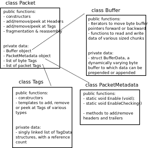
Implementation overview of Packet class.
Figure Implementation overview of Packet class. is a high-level overview of the Packet implementation; more detail on the byte Buffer implementation is provided later in Figure Implementation overview of a packet’s byte Buffer.. In ns-3, the Packet byte buffer is analogous to a Linux skbuff or BSD mbuf; it is a serialized representation of the actual data in the packet. The tag lists are containers for extra items useful for simulation convenience; if a Packet is converted to an emulated packet and put over an actual network, the tags are stripped off and the byte buffer is copied directly into a real packet.
Packets are reference counted objects. They are handled with smart pointer (Ptr) objects like many of the objects in the ns-3 system. One small difference you will see is that class Packet does not inherit from class Object or class RefCountBase, and implements the Ref() and Unref() methods directly. This was designed to avoid the overhead of a vtable in class Packet.
The Packet class is designed to be copied cheaply; the overall design is based on Copy on Write (COW). When there are multiple references to a packet object, and there is an operation on one of them, only so-called “dirty” operations will trigger a deep copy of the packet:
ns3::Packet::AddHeader()ns3::Packet::AddTrailer()both versions of ns3::Packet::AddAtEnd()Packet::RemovePacketTag()
The fundamental classes for adding to and removing from the byte buffer are
class Header and class Trailer. Headers are more common but the below
discussion also largely applies to protocols using trailers. Every protocol
header that needs to be inserted and removed from a Packet instance should
derive from the abstract Header base class and implement the private pure
virtual methods listed below:
ns3::Header::SerializeTo()ns3::Header::DeserializeFrom()ns3::Header::GetSerializedSize()ns3::Header::PrintTo()
Basically, the first three functions are used to serialize and deserialize
protocol control information to/from a Buffer. For example, one may define
class TCPHeader : public Header. The TCPHeader object will typically
consist of some private data (like a sequence number) and public interface
access functions (such as checking the bounds of an input). But the underlying
representation of the TCPHeader in a Packet Buffer is 20 serialized bytes (plus
TCP options). The TCPHeader::SerializeTo() function would therefore be designed
to write these 20 bytes properly into the packet, in network byte order. The
last function is used to define how the Header object prints itself onto an
output stream.
Similarly, user-defined Tags can be appended to the packet. Unlike Headers, Tags are not serialized into a contiguous buffer but are stored in lists. Tags can be flexibly defined to be any type, but there can only be one instance of any particular object type in the Tags buffer at any time.
Using the packet interface
This section describes how to create and use the ns3::Packet object.
Creating a new packet
The following command will create a new packet with a new unique Id.:
Ptr<Packet> pkt = Create<Packet> ();
What is the Uid (unique Id)? It is an internal id that the system uses to identify packets. It can be fetched via the following method:
uint32_t uid = pkt->GetUid ();
But please note the following. This uid is an internal uid and cannot be counted on to provide an accurate counter of how many “simulated packets” of a particular protocol are in the system. It is not trivial to make this uid into such a counter, because of questions such as what should the uid be when the packet is sent over broadcast media, or when fragmentation occurs. If a user wants to trace actual packet counts, he or she should look at e.g. the IP ID field or transport sequence numbers, or other packet or frame counters at other protocol layers.
We mentioned above that it is possible to create packets with zero-filled payloads that do not actually require a memory allocation (i.e., the packet may behave, when delays such as serialization or transmission delays are computed, to have a certain number of payload bytes, but the bytes will only be allocated on-demand when needed). The command to do this is, when the packet is created:
Ptr<Packet> pkt = Create<Packet> (N);
where N is a positive integer.
The packet now has a size of N bytes, which can be verified by the GetSize() method:
/**
* \returns the size in bytes of the packet (including the zero-filled
* initial payload)
*/
uint32_t GetSize (void) const;
You can also initialize a packet with a character buffer. The input data is copied and the input buffer is untouched. The constructor applied is:
Packet (uint8_t const *buffer, uint32_t size);
Here is an example:
Ptr<Packet> pkt1 = Create<Packet> (reinterpret_cast<const uint8_t*> ("hello"), 5);
Packets are freed when there are no more references to them, as with all ns-3 objects referenced by the Ptr class.
Adding and removing Buffer data
After the initial packet creation (which may possibly create some fake initial bytes of payload), all subsequent buffer data is added by adding objects of class Header or class Trailer. Note that, even if you are in the application layer, handling packets, and want to write application data, you write it as an ns3::Header or ns3::Trailer. If you add a Header, it is prepended to the packet, and if you add a Trailer, it is added to the end of the packet. If you have no data in the packet, then it makes no difference whether you add a Header or Trailer. Since the APIs and classes for header and trailer are pretty much identical, we’ll just look at class Header here.
The first step is to create a new header class. All new Header classes must inherit from class Header, and implement the following methods:
Serialize ()Deserialize ()GetSerializedSize ()Print ()
To see a simple example of how these are done, look at the UdpHeader class headers src/internet/model/udp-header.cc. There are many other examples within the source code.
Once you have a header (or you have a preexisting header), the following Packet API can be used to add or remove such headers.:
/**
* Add header to this packet. This method invokes the
* Header::GetSerializedSize and Header::Serialize
* methods to reserve space in the buffer and request the
* header to serialize itself in the packet buffer.
*
* \param header a reference to the header to add to this packet.
*/
void AddHeader (const Header & header);
/**
* Deserialize and remove the header from the internal buffer.
*
* This method invokes Header::Deserialize (begin) and should be used for
* fixed-length headers.
*
* \param header a reference to the header to remove from the internal buffer.
* \returns the number of bytes removed from the packet.
*/
uint32_t RemoveHeader (Header &header);
/**
* Deserialize but does _not_ remove the header from the internal buffer.
* This method invokes Header::Deserialize.
*
* \param header a reference to the header to read from the internal buffer.
* \returns the number of bytes read from the packet.
*/
uint32_t PeekHeader (Header &header) const;
For instance, here are the typical operations to add and remove a UDP header.:
// add header
Ptr<Packet> packet = Create<Packet> ();
UdpHeader udpHeader;
// Fill out udpHeader fields appropriately
packet->AddHeader (udpHeader);
...
// remove header
UdpHeader udpHeader;
packet->RemoveHeader (udpHeader);
// Read udpHeader fields as needed
If the header is variable-length, then another variant of RemoveHeader() is needed:
/**
* \brief Deserialize and remove the header from the internal buffer.
*
* This method invokes Header::Deserialize (begin, end) and should be
* used for variable-length headers (where the size is determined somehow
* by the caller).
*
* \param header a reference to the header to remove from the internal buffer.
* \param size number of bytes to deserialize
* \returns the number of bytes removed from the packet.
*/
uint32_t RemoveHeader (Header &header, uint32_t size);
In this case, the caller must figure out and provide the right ‘size’ as an argument (the Deserialization routine may not know when to stop). An example of this type of header would be a series of Type-Length-Value (TLV) information elements, where the ending point of the series of TLVs can be deduced from the packet length.
Adding and removing Tags
There is a single base class of Tag that all packet tags must derive from. They are used in two different tag lists in the packet; the lists have different semantics and different expected use cases.
As the names imply, ByteTags follow bytes and PacketTags follow packets. What this means is that when operations are done on packets, such as fragmentation, concatenation, and appending or removing headers, the byte tags keep track of which packet bytes they cover. For instance, if a user creates a TCP segment, and applies a ByteTag to the segment, each byte of the TCP segment will be tagged. However, if the next layer down inserts an IPv4 header, this ByteTag will not cover those bytes. The converse is true for the PacketTag; it covers a packet despite the operations on it.
Each tag type must subclass ns3::Tag, and only one instance of
each Tag type may be in each tag list. Here are a few differences in the
behavior of packet tags and byte tags.
- Fragmentation: As mentioned above, when a packet is fragmented, each packet fragment (which is a new packet) will get a copy of all packet tags, and byte tags will follow the new packet boundaries (i.e. if the fragmented packets fragment across a buffer region covered by the byte tag, both packet fragments will still have the appropriate buffer regions byte tagged).
- Concatenation: When packets are combined, two different buffer regions will become one. For byte tags, the byte tags simply follow the respective buffer regions. For packet tags, only the tags on the first packet survive the merge.
- Finding and Printing: Both classes allow you to iterate over all of the tags and print them.
- Removal: Users can add and remove the same packet tag multiple times on a single packet (AddPacketTag () and RemovePacketTag ()). The packet However, once a byte tag is added, it can only be removed by stripping all byte tags from the packet. Removing one of possibly multiple byte tags is not supported by the current API.
If a user wants to take an existing packet object and reuse it as a new packet, he or she should remove all byte tags and packet tags before doing so. An example is the UdpEchoServer class, which takes the received packet and “turns it around” to send back to the echo client.
The Packet API for byte tags is given below.:
/**
* \param tag the new tag to add to this packet
*
* Tag each byte included in this packet with the
* new tag.
*
* Note that adding a tag is a const operation which is pretty
* un-intuitive. The rationale is that the content and behavior of
* a packet is _not_ changed when a tag is added to a packet: any
* code which was not aware of the new tag is going to work just
* the same if the new tag is added. The real reason why adding a
* tag was made a const operation is to allow a trace sink which gets
* a packet to tag the packet, even if the packet is const (and most
* trace sources should use const packets because it would be
* totally evil to allow a trace sink to modify the content of a
* packet).
*/
void AddByteTag (const Tag &tag) const;
/**
* \returns an iterator over the set of byte tags included in this packet.
*/
ByteTagIterator GetByteTagIterator (void) const;
/**
* \param tag the tag to search in this packet
* \returns true if the requested tag type was found, false otherwise.
*
* If the requested tag type is found, it is copied in the user's
* provided tag instance.
*/
bool FindFirstMatchingByteTag (Tag &tag) const;
/**
* Remove all the tags stored in this packet.
*/
void RemoveAllByteTags (void);
/**
* \param os output stream in which the data should be printed.
*
* Iterate over the tags present in this packet, and
* invoke the Print method of each tag stored in the packet.
*/
void PrintByteTags (std::ostream &os) const;
The Packet API for packet tags is given below.:
/**
* \param tag the tag to store in this packet
*
* Add a tag to this packet. This method calls the
* Tag::GetSerializedSize and, then, Tag::Serialize.
*
* Note that this method is const, that is, it does not
* modify the state of this packet, which is fairly
* un-intuitive.
*/
void AddPacketTag (const Tag &tag) const;
/**
* \param tag the tag to remove from this packet
* \returns true if the requested tag is found, false
* otherwise.
*
* Remove a tag from this packet. This method calls
* Tag::Deserialize if the tag is found.
*/
bool RemovePacketTag (Tag &tag);
/**
* \param tag the tag to search in this packet
* \returns true if the requested tag is found, false
* otherwise.
*
* Search a matching tag and call Tag::Deserialize if it is found.
*/
bool PeekPacketTag (Tag &tag) const;
/**
* Remove all packet tags.
*/
void RemoveAllPacketTags (void);
/**
* \param os the stream in which we want to print data.
*
* Print the list of 'packet' tags.
*
* \sa Packet::AddPacketTag, Packet::RemovePacketTag, Packet::PeekPacketTag,
* Packet::RemoveAllPacketTags
*/
void PrintPacketTags (std::ostream &os) const;
/**
* \returns an object which can be used to iterate over the list of
* packet tags.
*/
PacketTagIterator GetPacketTagIterator (void) const;
Here is a simple example illustrating the use of tags from the
code in src/internet/model/udp-socket-impl.cc:
Ptr<Packet> p; // pointer to a pre-existing packet
SocketIpTtlTag tag
tag.SetTtl (m_ipMulticastTtl); // Convey the TTL from UDP layer to IP layer
p->AddPacketTag (tag);
This tag is read at the IP layer, then stripped (src/internet/model/ipv4-l3-protocol.cc):
uint8_t ttl = m_defaultTtl;
SocketIpTtlTag tag;
bool found = packet->RemovePacketTag (tag);
if (found)
{
ttl = tag.GetTtl ();
}
Fragmentation and concatenation
Packets may be fragmented or merged together. For example, to fragment a packet
p of 90 bytes into two packets, one containing the first 10 bytes and the
other containing the remaining 80, one may call the following code:
Ptr<Packet> frag0 = p->CreateFragment (0, 10);
Ptr<Packet> frag1 = p->CreateFragment (10, 90);
As discussed above, the packet tags from p will follow to both packet
fragments, and the byte tags will follow the byte ranges as needed.
Now, to put them back together:
frag0->AddAtEnd (frag1);
Now frag0 should be equivalent to the original packet p. If, however, there
were operations on the fragments before being reassembled (such as tag
operations or header operations), the new packet will not be the same.
Enabling metadata
We mentioned above that packets, being on-the-wire representations of byte buffers, present a problem to print out in a structured way unless the printing function has access to the context of the header. For instance, consider a tcpdump-like printer that wants to pretty-print the contents of a packet.
To enable this usage, packets may have metadata enabled (disabled by default for
performance reasons). This class is used by the Packet class to record every
operation performed on the packet’s buffer, and provides an implementation of
Packet::Print () method that uses the metadata to analyze the content of the
packet’s buffer.
The metadata is also used to perform extensive sanity checks at runtime when performing operations on a Packet. For example, this metadata is used to verify that when you remove a header from a packet, this same header was actually present at the front of the packet. These errors will be detected and will abort the program.
To enable this operation, users will typically insert one or both of these statements at the beginning of their programs:
Packet::EnablePrinting ();
Packet::EnableChecking ();
Sample programs
See src/network/examples/main-packet-header.cc and src/network/examples/main-packet-tag.cc.
Implementation details
Private member variables
A Packet object’s interface provides access to some private data:
Buffer m_buffer;
ByteTagList m_byteTagList;
PacketTagList m_packetTagList;
PacketMetadata m_metadata;
mutable uint32_t m_refCount;
static uint32_t m_globalUid;
Each Packet has a Buffer and two Tags lists, a PacketMetadata object, and a ref count. A static member variable keeps track of the UIDs allocated. The actual uid of the packet is stored in the PacketMetadata.
Note: that real network packets do not have a UID; the UID is therefore an instance of data that normally would be stored as a Tag in the packet. However, it was felt that a UID is a special case that is so often used in simulations that it would be more convenient to store it in a member variable.
Buffer implementation
Class Buffer represents a buffer of bytes. Its size is automatically adjusted to hold any data prepended or appended by the user. Its implementation is optimized to ensure that the number of buffer resizes is minimized, by creating new Buffers of the maximum size ever used. The correct maximum size is learned at runtime during use by recording the maximum size of each packet.
Authors of new Header or Trailer classes need to know the public API of the Buffer class. (add summary here)
The byte buffer is implemented as follows:
struct BufferData {
uint32_t m_count;
uint32_t m_size;
uint32_t m_initialStart;
uint32_t m_dirtyStart;
uint32_t m_dirtySize;
uint8_t m_data[1];
};
struct BufferData *m_data;
uint32_t m_zeroAreaSize;
uint32_t m_start;
uint32_t m_size;
BufferData::m_count: reference count for BufferData structureBufferData::m_size: size of data buffer stored in BufferData structureBufferData::m_initialStart: offset from start of data buffer where data was first insertedBufferData::m_dirtyStart: offset from start of buffer where every Buffer which holds a reference to this BufferData instance have written data so farBufferData::m_dirtySize: size of area where data has been written so farBufferData::m_data: pointer to data bufferBuffer::m_zeroAreaSize: size of zero area which extends beforem_initialStartBuffer::m_start: offset from start of buffer to area used by this bufferBuffer::m_size: size of area used by this Buffer in its BufferData structure
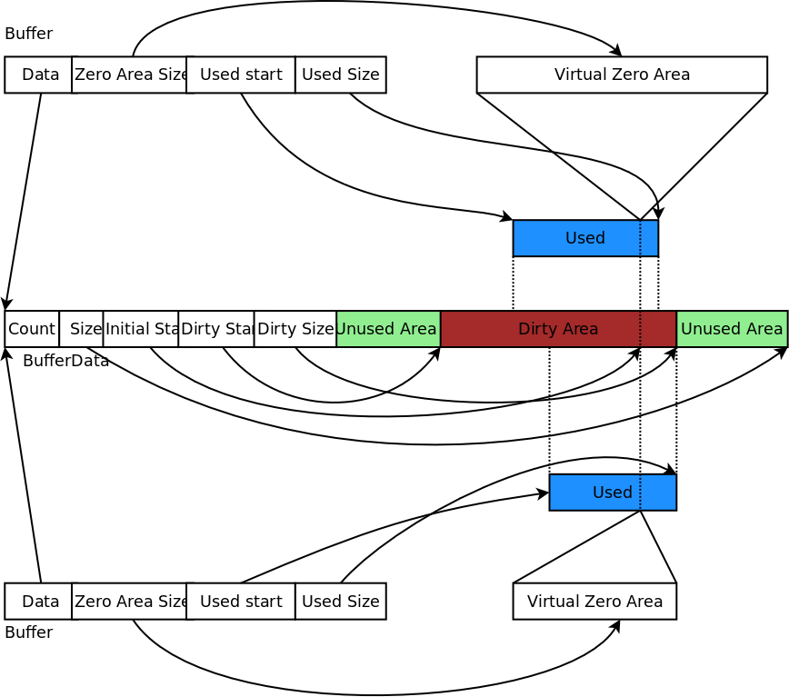
Implementation overview of a packet’s byte Buffer.
This data structure is summarized in Figure Implementation overview of a packet’s byte Buffer.. Each Buffer holds a pointer to an instance of a BufferData. Most Buffers should be able to share the same underlying BufferData and thus simply increase the BufferData’s reference count. If they have to change the content of a BufferData inside the Dirty Area, and if the reference count is not one, they first create a copy of the BufferData and then complete their state-changing operation.
Tags implementation
(XXX revise me)
Tags are implemented by a single pointer which points to the start of a linked list ofTagData data structures. Each TagData structure points to the next TagData in the list (its next pointer contains zero to indicate the end of the linked list). Each TagData contains an integer unique id which identifies the type of the tag stored in the TagData.:
struct TagData {
struct TagData *m_next;
uint32_t m_id;
uint32_t m_count;
uint8_t m_data[Tags::SIZE];
};
class Tags {
struct TagData *m_next;
};
Adding a tag is a matter of inserting a new TagData at the head of the linked list. Looking at a tag requires you to find the relevant TagData in the linked list and copy its data into the user data structure. Removing a tag and updating the content of a tag requires a deep copy of the linked list before performing this operation. On the other hand, copying a Packet and its tags is a matter of copying the TagData head pointer and incrementing its reference count.
Tags are found by the unique mapping between the Tag type and its underlying id. This is why at most one instance of any Tag can be stored in a packet. The mapping between Tag type and underlying id is performed by a registration as follows:
/* A sample Tag implementation
*/
struct MyTag {
uint16_t m_streamId;
};
Memory management
Describe dataless vs. data-full packets.
Copy-on-write semantics
The current implementation of the byte buffers and tag list is based on COW (Copy On Write). An introduction to COW can be found in Scott Meyer’s “More Effective C++”, items 17 and 29). This design feature and aspects of the public interface borrows from the packet design of the Georgia Tech Network Simulator. This implementation of COW uses a customized reference counting smart pointer class.
What COW means is that copying packets without modifying them is very cheap (in terms of CPU and memory usage) and modifying them can be also very cheap. What is key for proper COW implementations is being able to detect when a given modification of the state of a packet triggers a full copy of the data prior to the modification: COW systems need to detect when an operation is “dirty” and must therefore invoke a true copy.
Dirty operations:
- ns3::Packet::AddHeader
- ns3::Packet::AddTrailer
- both versions of ns3::Packet::AddAtEnd
- ns3::Packet::RemovePacketTag
Non-dirty operations:
- ns3::Packet::AddPacketTag
- ns3::Packet::PeekPacketTag
- ns3::Packet::RemoveAllPacketTags
- ns3::Packet::AddByteTag
- ns3::Packet::FindFirstMatchingByteTag
- ns3::Packet::RemoveAllByteTags
- ns3::Packet::RemoveHeader
- ns3::Packet::RemoveTrailer
- ns3::Packet::CreateFragment
- ns3::Packet::RemoveAtStart
- ns3::Packet::RemoveAtEnd
- ns3::Packet::CopyData
Dirty operations will always be slower than non-dirty operations, sometimes by several orders of magnitude. However, even the dirty operations have been optimized for common use-cases which means that most of the time, these operations will not trigger data copies and will thus be still very fast.
Error Model
This section documents a few error model objects, typically associated with
NetDevice models, that are maintained as part of the network module:
- RateErrorModel
- ListErrorModel
- ReceiveListErrorModel
- BurstErrorModel
Error models are used to indicate that a packet should be considered to be errored, according to the underlying (possibly stochastic or empirical) error model.
Model Description
The source code for error models live in the directory src/packet/utils.
Two types of error models are generally provided. The first are stochastic
models. In this case, packets are errored according to underlying
random variable distributions. An example of this is the RateErrorModel.
The other type of model is a deterministic or empirical model, in which
packets are errored according to a particular prescribed pattern.
An example is the ListErrorModel that allows users to specify
the list of packets to be errored, by listing the specific packet UIDs.
The ns3::RateErrorModel errors packets according to an underlying
random variable distribution, which is by default a UniformRandomVariable
distributed between 0.0 and 1.0. The error rate and error units (bit,
byte, or packet) are set by the user. For instance, by setting ErrorRate
to 0.1 and ErrorUnit to “Packet”, in the long run, around 10% of the
packets will be lost.
Design
Error models are ns-3 objects and can be created using the typical
pattern of CreateObject<>(). They have configuration attributes.
An ErrorModel can be applied anywhere, but are commonly deployed on NetDevice models so that artificial losses (mimicking channel losses) can be induced.
Scope and Limitations
No known limitations. There are no existing models that try to modify the packet contents (e.g. apply bit or byte errors to the byte buffers). This type of operation will likely be performance-expensive, and existing Packet APIs may not easily support it.
The ns-3 spectrum model and devices that derive from it (e.g. LTE) have their own error model base class, found in
References
The initial ns-3 error models were ported from ns-2 (queue/errmodel.{cc,h})
Usage
The base class API is as follows:
bool ErrorModel::IsCorrupt (Ptr<Packet> pkt): Evaluate the packet and return true or false whether the packet should be considered errored or not. Some models could potentially alter the contents of the packet bit buffer.void ErrorModel::Reset (void): Reset any state.void ErrorModel::Enable (void): Enable the modelvoid ErrorModel::Disble (void): Disable the model; IsCorrupt() will always return false.bool ErrorModel::IsEnabled (void) const: Return the enabled state
Many ns-3 NetDevices contain attributes holding pointers to error
models. The error model is applied in the notional physical layer
processing chain of the device, and drops should show up on the PhyRxDrop
trace source of the device. The following are known to include an attribute
with a pointer available to hold this type of error model:
SimpleNetDevicePointToPointNetDeviceCsmaNetDeviceVirtualNetDevice
However, the ErrorModel could be used anywhere where packets are used
Helpers
This model is typically not used with helpers.
Attributes
The RateErrorModel contains the following attributes:
Output
What kind of data does the model generate? What are the key trace sources? What kind of logging output can be enabled?
Examples
Error models are used in the tutorial fifth and sixth programs.
The directory examples/error-model/ contains an example
simple-error-model.cc that exercises the Rate and List error models.
The TCP example examples/tcp/tcp-nsc-lfn.cc uses the Rate error model.
Troubleshooting
No known issues.
Validation
The error-model unit test suite provides a single test case of
of a particular combination of ErrorRate and ErrorUnit for the
RateErrorModel applied to a SimpleNetDevice.
Acknowledgements
The basic ErrorModel, RateErrorModel, and ListErrorModel classes were ported from ns-2 to ns-3 in 2007. The ReceiveListErrorModel was added at that time.
The burst error model is due to Truc Anh N. Nguyen at the University of Kansas (James P.G. Sterbenz <jpgs@ittc.ku.edu>, director, ResiliNets Research Group (http://wiki.ittc.ku.edu/resilinets), Information and Telecommunication Technology Center (ITTC) and Department of Electrical Engineering and Computer Science, The University of Kansas Lawrence, KS USA). Work supported in part by NSF FIND (Future Internet Design) Program under grant CNS-0626918 (Postmodern Internet Architecture), NSF grant CNS-1050226 (Multilayer Network Resilience Analysis and Experimentation on GENI), US Department of Defense (DoD), and ITTC at The University of Kansas.
Node and NetDevices Overview
This chapter describes how ns-3 nodes are put together, and provides a walk-through of how packets traverse an internet-based Node.
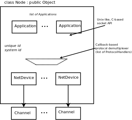
High-level node architecture
In ns-3, nodes are instances of ns3::Node. This class may be
subclassed, but instead, the conceptual model is that we aggregate or insert
objects to it rather than define subclasses.
One might think of a bare ns-3 node as a shell of a computer, to which one may
add NetDevices (cards) and other innards including the protocols and
applications. High-level node architecture illustrates that ns3::Node
objects contain a list of ns3::Application instances (initially,
the list is empty), a list of ns3::NetDevice instances (initially,
the list is empty), a list of ns3::Node::ProtocolHandler instances,
a unique integer ID, and a system ID (for distributed simulation).
The design tries to avoid putting too many dependencies on the class
ns3::Node, ns3::Application, or
ns3::NetDevice for the following:
- IP version, or whether IP is at all even used in the
ns3::Node. - implementation details of the IP stack.
From a software perspective, the lower interface of applications corresponds to
the C-based sockets API. The upper interface of ns3::NetDevice
objects corresponds to the device independent sublayer of the Linux stack.
Everything in between can be aggregated and plumbed together as needed.
Let’s look more closely at the protocol demultiplexer. We want incoming frames at layer-2 to be delivered to the right layer-3 protocol such as IPv4. The function of this demultiplexer is to register callbacks for receiving packets. The callbacks are indexed based on the EtherType in the layer-2 frame.
Many different types of higher-layer protocols may be connected to the NetDevice, such as IPv4, IPv6, ARP, MPLS, IEEE 802.1x, and packet sockets. Therefore, the use of a callback-based demultiplexer avoids the need to use a common base class for all of these protocols, which is problematic because of the different types of objects (including packet sockets) expected to be registered there.
Sockets APIs
The sockets API is a long-standing API used by user-space applications to access network services in the kernel. A socket is an abstraction, like a Unix file handle, that allows applications to connect to other Internet hosts and exchange reliable byte streams and unreliable datagrams, among other services.
ns-3 provides two types of sockets APIs, and it is important to understand the differences between them. The first is a native ns-3 API, while the second uses the services of the native API to provide a POSIX-like API as part of an overall application process. Both APIs strive to be close to the typical sockets API that application writers on Unix systems are accustomed to, but the POSIX variant is much closer to a real system’s sockets API.
ns-3 sockets API
The native sockets API for ns-3 provides an interface to various types of transport protocols (TCP, UDP) as well as to packet sockets and, in the future, Netlink-like sockets. However, users are cautioned to understand that the semantics are not the exact same as one finds in a real system (for an API which is very much aligned to real systems, see the next section).
ns3::Socket is defined in src/network/model/socket.h.
Readers will note that many public member functions are aligned
with real sockets function calls, and all other things being equal,
we have tried to align with a Posix sockets API. However, note that:
- ns-3 applications handle a smart pointer to a Socket object, not a file descriptor;
- there is no notion of synchronous API or a blocking API; in fact, the model for interaction between application and socket is one of asynchronous I/O, which is not typically found in real systems (more on this below);
- the C-style socket address structures are not used;
- the API is not a complete sockets API, such as supporting all socket options or all function variants;
- many calls use
ns3::Packetclass to transfer data between application and socket. This may seem peculiar to pass Packets across a stream socket API, but think of these packets as just fancy byte buffers at this level (more on this also below).
Basic operation and calls
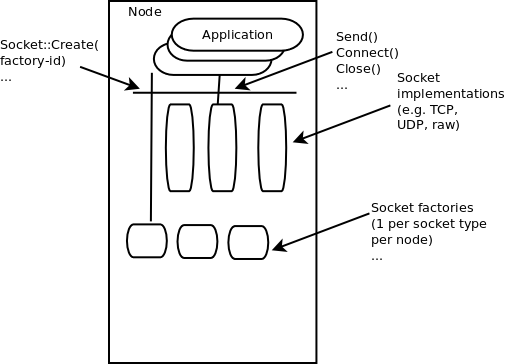
Implementation overview of native sockets API
Creating sockets
An application that wants to use sockets must first create one.
On real systems using a C-based API, this is accomplished by calling socket()
int socket(int domain, int type, int protocol);
which creates a socket in the system and returns an integer descriptor.
In ns-3, we have no equivalent of a system call at the lower layers, so we adopt the following model. There are certain factory objects that can create sockets. Each factory is capable of creating one type of socket, and if sockets of a particular type are able to be created on a given node, then a factory that can create such sockets must be aggregated to the Node:
static Ptr<Socket> CreateSocket (Ptr<Node> node, TypeId tid);
Examples of TypeIds to pass to this method are ns3::TcpSocketFactory,
ns3::PacketSocketFactory, and ns3::UdpSocketFactory.
This method returns a smart pointer to a Socket object. Here is an example:
Ptr<Node> n0;
// Do some stuff to build up the Node's internet stack
Ptr<Socket> localSocket =
Socket::CreateSocket (n0, TcpSocketFactory::GetTypeId ());
In some ns-3 code, sockets will not be explicitly created by user’s
main programs, if an ns-3 application does it. For instance, for
ns3::OnOffApplication, the function ns3::OnOffApplication::StartApplication()
performs the socket creation, and the application holds the socket
pointer.
Using sockets
Below is a typical sequence of socket calls for a TCP client in a real implementation:
sock = socket(PF_INET, SOCK_STREAM, IPPROTO_TCP);
bind(sock, ...);
connect(sock, ...);
send(sock, ...);
recv(sock, ...);
close(sock);
There are analogs to all of these calls in ns-3, but we will focus on two aspects here. First, most usage of sockets in real systems requires a way to manage I/O between the application and kernel. These models include blocking sockets, signal-based I/O, and non-blocking sockets with polling. In ns-3, we make use of the callback mechanisms to support a fourth mode, which is analogous to POSIX asynchronous I/O.
In this model, on the sending side, if the send() call were to
fail because of insufficient buffers, the application suspends the
sending of more data until a function registered at the
ns3::Socket::SetSendCallback() callback is invoked.
An application can also ask the socket how much space is available
by calling ns3::Socket::GetTxAvailable(). A typical sequence
of events for sending data (ignoring connection setup) might be:
SetSendCallback (MakeCallback(&HandleSendCallback));
Send ();
Send ();
...
// Send fails because buffer is full
// Wait until HandleSendCallback is called
// HandleSendCallback is called by socket, since space now available
Send (); // Start sending again
Similarly, on the receive side, the socket user does not block on
a call to recv(). Instead, the application sets a callback
with ns3::Socket::SetRecvCallback() in which the socket will notify the
application when (and how much) there is data to be read, and
the application then calls ns3::Socket::Recv() to read the data until
no more can be read.
Packet vs. buffer variants
There are two basic variants of Send() and Recv() supported:
virtual int Send (Ptr<Packet> p) = 0;
int Send (const uint8_t* buf, uint32_t size);
Ptr<Packet> Recv (void);
int Recv (uint8_t* buf, uint32_t size);
The non-Packet variants are provided for legacy API reasons. When calling
the raw buffer variant of ns3::Socket::Send(), the buffer is immediately
written into a Packet and the packet variant is invoked.
Users may find it semantically odd to pass a Packet to a stream socket
such as TCP. However, do not let the name bother you; think of
ns3::Packet to be a fancy byte buffer. There are a few reasons why
the Packet variants are more likely to be preferred in ns-3:
- Users can use the Tags facility of packets to, for example, encode a flow ID or other helper data at the application layer.
- Users can exploit the copy-on-write implementation to avoid
memory copies (on the receive side, the conversion back to a
uint8_t* bufmay sometimes incur an additional copy). - Use of Packet is more aligned with the rest of the ns-3 API
Sending dummy data
Sometimes, users want the simulator to just pretend that there is an
actual data payload in the packet (e.g. to calculate transmission delay)
but do not want to actually produce or consume the data. This is
straightforward to support in ns-3; have applications call
Create<Packet> (size); instead of Create<Packet> (buffer, size);.
Similarly, passing in a zero to the pointer argument in the raw buffer
variants has the same effect. Note that, if some subsequent code tries
to read the Packet data buffer, the fake buffer will be converted to
a real (zeroed) buffer on the spot, and the efficiency will be lost there.
Use of Send() vs. SendTo()
There are two variants of methods used to send data to the socket:
virtual int Send (Ptr<Packet> p, uint32_t flags) = 0;
virtual int SendTo (Ptr<Packet> p, uint32_t flags,
const Address &toAddress) = 0;
The first method is used if the socket has already been connected
(Socket::Connect()) to a peer address. In the case of stream-based
sockets like TCP, the connect call is required to bind the socket to
a peer address, and thereafter, Send() is typically used. In the case of
datagram-based sockets like UDP, the socket is not required to
be connected to a peer address before sending, and the socket may be used to
send data to different destination addresses; in this case, the
SendTo() method is used to specify the destination address for
the datagram.
Socket options
ToS (Type of Service)
The native sockets API for ns-3 provides two public methods (of the Socket base class):
void SetIpTos (uint8_t ipTos);
uint8_t GetIpTos (void) const;
to set and get, respectively, the type of service associated with the socket.
These methods are equivalent to using the IP_TOS option of BSD sockets.
Clearly, setting the type of service only applies to sockets using the IPv4 protocol.
However, users typically do not set the type of service associated with a socket
through ns3::Socket::SetIpTos() because sockets are normally created
by application helpers and users cannot get a pointer to the sockets.
Instead, users can create an address of type ns3::InetSocketAddress
with the desired type of service value and pass it to the application helpers:
InetSocketAddress destAddress (ipv4Address, udpPort);
destAddress.SetTos (tos);
OnOffHelper onoff ("ns3::UdpSocketFactory", destAddress);
For this to work, the application must eventually call the
ns3::Socket::Connect() method to connect to the provided
destAddress and the Connect method of the particular socket type must
support setting the type of service associated with a socket (by using
the ns3::Socket::SetIpTos() method). Currently, the socket
types that support setting the type of service in such a way are
ns3::UdpSocketImpl and ns3::TcpSocketBase.
The type of service associated with a socket is then used to determine the value of the Type of Service field (renamed as Differentiated Services field by RFC 2474) of the IPv4 header of the packets sent through that socket, as detailed in the next sections.
Setting the ToS with UDP sockets
For IPv4 packets, the ToS field is set according to the following rules:
- If the socket is connected, the ToS field is set to the ToS value associated with the socket.
- If the socket is not connected, the ToS field is set to the value specified
in the destination address (of type
ns3::InetSocketAddress) passed tons3::Socket::SendTo(), and the ToS value associated with the socket is ignored.
Setting the ToS with TCP sockets
For IPv4 packets, the ToS field is set to the ToS value associated with the socket.
Priority
The native sockets API for ns-3 provides two public methods (of the Socket base class):
void SetPriority (uint8_t priority);
uint8_t GetPriority (void) const;
to set and get, respectively, the priority associated with the socket. These methods are equivalent to using the SO_PRIORITY option of BSD sockets. Only values in the range 0..6 can be set through the above method.
Note that setting the type of service associated with a socket (by calling
ns3::Socket::SetIpTos()) also sets the priority for the socket
to the value that the ns3::Socket::IpTos2Priority() function
returns when it is passed the type of service value. This function
is implemented after the Linux rt_tos2priority function, which takes
an 8-bit value as input and returns a value which is a function of bits 3-6
(where bit 0 is the most significant bit) of the input value:
| Bits 3-6 | Priority |
|---|---|
| 0 to 3 | 0 (Best Effort) |
| 4 to 7 | 2 (Bulk) |
| 8 to 11 | 6 (Interactive) |
| 12 to 15 | 4 (Interactive Bulk) |
The rationale is that bits 3-6 of the Type of Service field were interpreted
as the TOS subfield by (the obsolete) RFC 1349. Readers can refer to the
doxygen documentation of ns3::Socket::IpTos2Priority()
for more information, including how DSCP values map onto priority values.
The priority set for a socket (as described above) is then used to determine
the priority of the packets sent through that socket, as detailed in the next
sections. Currently, the socket types that support setting the packet priority
are ns3::UdpSocketImpl, ns3::TcpSocketBase and
ns3::PacketSocket. The packet priority is used, e.g., by queuing
disciplines such as the default PfifoFastQueueDisc to classify packets into
distinct queues.
Setting the priority with UDP sockets
If the packet is an IPv4 packet and the value to be inserted in the ToS field
is not null, then the packet is assigned a priority based on such ToS value
(according to the ns3::Socket::IpTos2Priority() function). Otherwise,
the priority associated with the socket is assigned to the packet.
Setting the priority with TCP sockets
Every packet is assigned a priority equal to the priority associated with the socket.
Setting the priority with packet sockets
Every packet is assigned a priority equal to the priority associated with the socket.
Socket errno
to be completed
Example programs
to be completed
POSIX-like sockets API
Simple NetDevice
Placeholder chapter
Queues
This section documents the queue object, which is typically used by NetDevices and QueueDiscs to store packets.
Packets stored in a queue can be managed according to different policies. Currently, only the DropTail policy is available.
Model Description
The source code for the new module lives in the directory src/network/utils.
ns3::Queue has been redesigned as a template class object to allow us to instantiate queues storing different types of items. The unique template type parameter specifies the type of items stored in the queue. The only requirement on the item type is that it must provide a GetSize () method which returns the size of the packet included in the item. Currently, queue items can be objects of the following classes:
- Packet
- QueueItem and subclasses (e.g., QueueDiscItem)
- WifiMacQueueItem
The internal queues of the queue discs are of type Queue<QueueDiscItem> (an alias of which being InternalQueue). A number of network devices (SimpleNetDevice, PointToPointNetDevice, CsmaNetDevice) use a Queue<Packet> to store packets to be transmitted. WifiNetDevices use instead queues of type WifiMacQueue, which is a subclass of Queue storing objects of type WifiMacQueueItem. Other devices, such as WiMax and LTE, use specialized queues.
Design
The Queue class derives from the QueueBase class, which is a non-template class providing all the methods that are independent of the type of the items stored in the queue. The Queue class provides instead all the operations that depend on the item type, such as enqueue, dequeue, peek and remove. The Queue class also provides the ability to trace certain queue operations such as enqueuing, dequeuing, and dropping.
Queue is an abstract base class and is subclassed for specific scheduling and drop policies. Subclasses need to define the following public methods:
bool Enqueue (Ptr<Item> item): Enqueue a packetPtr<Item> Dequeue (void): Dequeue a packetPtr<Item> Remove (void): Remove a packetPtr<const Item> Peek (void): Peek a packet
The Enqueue method does not allow to store a packet if the queue capacity is exceeded. Subclasses may also define specialized public methods. For instance, the WifiMacQueue class provides a method to dequeue a packet based on its tid and MAC address.
There are five trace sources that may be hooked:
EnqueueDequeueDropDropBeforeEnqueueDropAfterDequeue
Also, the QueueBase class defines two additional trace sources:
PacketsInQueueBytesInQueue
DropTail
This is a basic first-in-first-out (FIFO) queue that performs a tail drop when the queue is full.
The DropTailQueue class defines one attribute:
MaxSize: the maximum queue size
Usage
Helpers
A typical usage pattern is to create a device helper and to configure the queue type and attributes from the helper, such as this example:
PointToPointHelper p2p;
p2p.SetQueue ("ns3::DropTailQueue");
p2p.SetDeviceAttribute ("DataRate", StringValue ("10Mbps"));
p2p.SetChannelAttribute ("Delay", StringValue ("2ms"));
NetDeviceContainer devn0n2 = p2p.Install (n0n2);
p2p.SetQueue ("ns3::DropTailQueue");
p2p.SetDeviceAttribute ("DataRate", StringValue ("10Mbps"));
p2p.SetChannelAttribute ("Delay", StringValue ("3ms"));
NetDeviceContainer devn1n2 = p2p.Install (n1n2);
p2p.SetQueue ("ns3::DropTailQueue",
"MaxSize", StringValue ("50p"));
p2p.SetDeviceAttribute ("DataRate", StringValue (linkDataRate));
p2p.SetChannelAttribute ("Delay", StringValue (linkDelay));
NetDeviceContainer devn2n3 = p2p.Install (n2n3);
Please note that the SetQueue method of the PointToPointHelper class allows to specify “ns3::DropTailQueue” instead of “ns3::DropTailQueue<Packet>”. The same holds for CsmaHelper, SimpleNetDeviceHelper and TrafficControlHelper.
Output
The ns-3 ascii trace helpers used by many of the NetDevices will hook
the Enqueue, Dequeue, and Drop traces of these queues and print out
trace statements, such as the following from examples/udp/udp-echo.cc:
+ 2 /NodeList/0/DeviceList/1/$ns3::CsmaNetDevice/TxQueue/Enqueue ns3::EthernetHeader
( length/type=0x806, source=00:00:00:00:00:01, destination=ff:ff:ff:ff:ff:ff)
ns3::ArpHeader (request source mac: 00-06-00:00:00:00:00:01 source ipv4: 10.1.1.1
dest ipv4: 10.1.1.2) Payload (size=18) ns3::EthernetTrailer (fcs=0)
- 2 /NodeList/0/DeviceList/1/$ns3::CsmaNetDevice/TxQueue/Dequeue ns3::EthernetHeader
( length/type=0x806, source=00:00:00:00:00:01, destination=ff:ff:ff:ff:ff:ff)
ns3::ArpHeader (request source mac: 00-06-00:00:00:00:00:01 source ipv4: 10.1.1.1
dest ipv4: 10.1.1.2) Payload (size=18) ns3::EthernetTrailer (fcs=0)
which shows an enqueue “+” and dequeue “-” event at time 2 seconds.
Users are, of course, free to define and hook their own trace sinks to these trace sources.
Examples
The drop-tail queue is used in several examples, such as
examples/udp/udp-echo.cc.
Queue limits
This section documents the queue limits model, which is used by the traffic control to limit the NetDevices queueing delay. It operates on the transmission path of the network node.
The reduction of the NetDevices queueing delay is essential to improve the effectiveness of Active Queue Management (AQM) algorithms. Careful assessment of the queueing delay includes a byte-based measure of the NetDevices queue length. In this design, traffic control can use different byte-based schemes to limit the queueing delay. Currently the only available scheme is DynamicQueueLimits, which is modelled after the dynamic queue limit library of Linux.
Model Description
The source code for the model lives in the directory src/network/utils.
The model allows a byte-based measure of the netdevice queue. The byte-based measure more accurately approximates the time required to empty the queue than a packet-based measure.
To inform the upper layers about the transmission of packets, NetDevices can call a couple of functions:
void NotifyQueuedBytes (uint32_t bytes): Report the number of bytes queued to the device queuevoid NotifyTransmittedBytes (uint32_t bytes): Report the number of bytes transmitted by device
Based on this information, the QueueLimits object can stop the transmission queue.
In case of multiqueue NetDevices this mechanism is available for each queue.
The QueueLimits model can be used on any NetDevice modelled in ns-3.
Design
An abstract base class, class QueueLimits, is subclassed for specific byte-based limiting strategies.
Common operations provided by the base class QueueLimits include:
void Reset (): Reset queue limits statevoid Completed (uint32_t count): Record the number of completed bytes and recalculate the limitint32_t Available () const: Return how many bytes can be queuedvoid Queued (uint32_t count): Record number of bytes queued
DynamicQueueLimits
Dynamic queue limits (DQL) is a basic library implemented in the Linux kernel to limit the Ethernet queueing delay. DQL is a general purpose queue length controller. The goal of DQL is to calculate the limit as the minimum number of bytes needed to prevent starvation.
Three attributes are defined in the DynamicQueueLimits class:
HoldTime: The DQL algorithm hold timeMaxLimit: Maximum limitMinLimit: Minimum limit
The DQL algorithm hold time is 1 s. Reducing the HoldTime increases the responsiveness of DQL with consequent greater number of limit variation events. Conversely, increasing the HoldTime decreases the responsiveness of DQL with a minor number of limit variation events. The limit calculated by DQL is in the range from MinLimit to MaxLimit. The default values are respectively 0 and DQL_MAX_LIMIT. Increasing the MinLimit is recommended in case of higher NetDevice transmission rate (e.g. 1 Gbps) while reducing the MaxLimit is recommended in case of lower NetDevice transmission rate (e.g. 500 Kbps).
There is one trace source in DynamicQueueLimits class that may be hooked:
Limit: Limit value calculated by DQL
Usage
Helpers
A typical usage pattern is to create a traffic control helper and configure the queue limits type and attributes from the helper, such as this example:
TrafficControlHelper tch;
uint32_t handle = tch.SetRootQueueDisc ("ns3::PfifoFastQueueDisc", "Limit", UintegerValue (1000));
tch.SetQueueLimits ("ns3::DynamicQueueLimits", "HoldTime", StringValue ("4ms"));
then install the configuration on a NetDevices container
tch.Install (devices);
Nix-Vector Routing Documentation
Nix-vector routing is a simulation specific routing protocol and is intended for large network topologies. The on-demand nature of this protocol as well as the low-memory footprint of the nix-vector provides improved performance in terms of memory usage and simulation run time when dealing with a large number of nodes.
Model Description
The source code for the NixVectorRouting module lives in
the directory src/nix-vector-routing.
ns-3 nix-vector-routing performs on-demand route computation using a breadth-first search and an efficient route-storage data structure known as a nix-vector.
When a packet is generated at a node for transmission, the route is calculated, and the nix-vector is built.
How is the Nix-Vector calculated? The nix-vector stores an index for each hop along the path, which corresponds to the neighbor-index. This index is used to determine which net-device and gateway should be used.
How does the routing take place? To route a packet, the nix-vector must be transmitted with the packet. At each hop, the current node extracts the appropriate neighbor-index from the nix-vector and transmits the packet through the corresponding net-device. This continues until the packet reaches the destination.
Note
Nix-Vector routing does not use any routing metrics (interface metrics) during the calculation of nix-vector. It is only based on the shortest path calculated according to BFS.
How does Nix decide between two equally short path from source to
destination?
It depends on how the topology is constructed i.e., the order in which the
net-devices are added on a node and net-devices added on the channels
associated with current node’s net-devices. Please check the nix-simple.cc
example below to understand how nix-vectors are calculated.
ns-3 supports IPv4 as well as IPv6 Nix-Vector routing.
Scope and Limitations
Currently, the ns-3 model of nix-vector routing supports IPv4 and IPv6 p2p links, CSMA links and multiple WiFi networks with the same channel object. It does not (yet) provide support for efficient adaptation to link failures. It simply flushes all nix-vector routing caches.
NixVectorRouting performs a subnet matching check, but it does not check entirely if the addresses have been appropriately assigned. In other terms, using Nix-Vector routing, it is possible to have a working network that violates some good practices in IP address assignments.
In case of IPv6, Nix assumes the link-local addresses assigned are unique. When using the IPv6 stack, the link-local address allocation is unique by default over the entire topology. However, if the link-local addresses are assigned manually, the user must ensure uniqueness of link-local addresses.
Usage
The usage pattern is the one of all the Internet routing protocols.
Since NixVectorRouting is not installed by default in the
Internet stack, it is necessary to set it in the Internet Stack
helper by using InternetStackHelper::SetRoutingHelper.
Remember to include the header file ns3/nix-vector-helper.h to
use IPv4 or IPv6 Nix-Vector routing.
Note
The previous header file ns3/ipv4-nix-vector-helper.h is
maintained for backward compatibility reasons. Therefore, the
existing IPv4 Nix-Vector routing simulations should work fine.
- Using IPv4 Nix-Vector Routing:
Ipv4NixVectorHelper nixRouting;
InternetStackHelper stack;
stack.SetRoutingHelper (nixRouting); // has effect on the next Install ()
stack.Install (allNodes); // allNodes is the NodeContainer
- Using IPv6 Nix-Vector Routing:
Ipv6NixVectorHelper nixRouting;
InternetStackHelper stack;
stack.SetRoutingHelper (nixRouting); // has effect on the next Install ()
stack.Install (allNodes); // allNodes is the NodeContainer
Note
The NixVectorHelper helper class helps to use NixVectorRouting functionality.
The NixVectorRouting model can also be used directly to use Nix-Vector routing.
To use it directly, the header file ns3/nix-vector-routing.h should be
included. The previous header file ns3/ipv4-nix-vector-routing.h is maintained
for backwards compatibility with any existing IPv4 Nix-Vector routing simulations.
Examples
The examples for the NixVectorRouting module lives in
the directory src/nix-vector-routing/examples.
There are examples which use both IPv4 and IPv6 networking.
- nix-simple.cc
/*
* ________
* / \
* n0 -- n1 -- n2 -- n3
*
* n0 IP: 10.1.1.1, 10.1.4.1
* n1 IP: 10.1.1.2, 10.1.2.1
* n2 IP: 10.1.2.2, 10.1.3.1, 10.1.4.2
* n3 IP: 10.1.3.2
*/
In this topology, we install Nix-Vector routing between source n0 and destination n3. The shortest possible route will be n0 -> n2 -> n3.
Let’s see how the nix-vector will be generated for this path:
n0 has 2 neighbors i.e. n1 and n3. n0 is connected to both using separate net-devices. But the net-device for n0 – n1 p2p link was created before the netdevice for n0 – n2 p2p link. Thus, n2 has neighbor-index of 1 (n1 has 0) with respect to n0.
n2 has 3 neighbors i.e. n1, n3 and n0. The n2 net-device for n1 – n2 p2p link was created before the n2 net-device for n2 – n3 p2p link which was before the n2 netdevice for n0 – n2 p2p link. This, n3 has neighbor-index of 01 (n1 has 00 and n0 has 10) with repect to n2.
Thus, the nix-vector for the path from n0 to n3 is 101.
Note
This neighbor-index or nix-index has total number of bits equal to minimum number of bits required to represent all the neighbors in their binary form.
Note
If there are multiple netdevices connected to the current netdevice on the channel then it depends on which order netdevices were added to the channel.
#. Using IPv4: .. code-block:: bash
# By default IPv4 network is selected ./waf –run src/nix-vector-routing/examples/nix-simple
#. Using IPv6: .. code-block:: bash
# Use the –useIPv6 flag ./waf –run “src/nix-vector-routing/examples/nix-simple –useIPv6”
- nms-p2p-nix.cc
This example demonstrates the advantage of Nix-Vector routing as Nix performs source-based routing (BFS) to have faster routing.
- nix-simple-multi-address.cc
This is an IPv4 example demonstrating multiple interface addresses. This example also shows how address assignment in between the simulation causes the all the route caches and Nix caches to flush.
# By default IPv4 network is selected
./waf --run src/nix-vector-routing/examples/nix-simple-multi-address
- nix-double-wifi.cc
This example demonstrates the working of Nix with two Wifi networks
operating on the same Wifi channel object. The example uses ns3::YansWifiChannel
for both the wifi networks.
#. Using IPv4: .. code-block:: bash
# By default IPv4 network is selected ./waf –run src/nix-vector-routing/examples/nix-double-wifi # Use the –enableNixLog to enable NixVectorRouting logging. ./waf –run “src/nix-vector-routing/examples/nix-double-wifi –enableNixLog”#. Using IPv6: .. code-block:: bash
# Use the –useIPv6 flag ./waf –run “src/nix-vector-routing/examples/nix-double-wifi –useIPv6” # Use the –enableNixLog to enable NixVectorRouting logging. ./waf –run “src/nix-vector-routing/examples/nix-double-wifi –useIPv6 –enableNixLog”
Optimized Link State Routing (OLSR)
This model implements the base specification of the Optimized Link State Routing (OLSR) protocol, which is a dynamic mobile ad hoc unicast routing protocol. It has been developed at the University of Murcia (Spain) by Francisco J. Ros for NS-2, and was ported to NS-3 by Gustavo Carneiro at INESC Porto (Portugal).
The implementation is based on OLSR Version 1 (RFC 3626 [rfc3626]) and it is not compliant with OLSR Version 2 (RFC 7181 [rfc7181]) or any of the Version 2 extensions.
Model Description
The source code for the OLSR model lives in the directory src/olsr. As stated before, the model is based on RFC 3626 ([rfc3626]). Moreover, many design choices are based on the previous ns2 model.
Scope and Limitations
The model is for IPv4 only.
- Mostly compliant with OLSR as documented in RFC 3626 ([rfc3626]),
- The use of multiple interfaces was not supported by the NS-2 version, but is supported in NS-3;
- OLSR does not respond to the routing event notifications corresponding to dynamic interface up and down (
ns3::RoutingProtocol::NotifyInterfaceUpandns3::RoutingProtocol::NotifyInterfaceDown) or address insertion/removalns3::RoutingProtocol::NotifyAddAddressandns3::RoutingProtocol::NotifyRemoveAddress). - Unlike the NS-2 version, does not yet support MAC layer feedback as described in RFC 3626 ([rfc3626]);
Host Network Association (HNA) is supported in this implementation
of OLSR. Refer to examples/olsr-hna.cc to see how the API
is used.
Usage
The usage pattern is the one of all the Internet routing protocols.
Since OLSR is not installed by default in the Internet stack, it is necessary to
set it in the Internet Stack helper by using InternetStackHelper::SetRoutingHelper
Typically, OLSR is enabled in a main program by use of an OlsrHelper class that installs OLSR into an Ipv4ListRoutingProtocol object. The following sample commands will enable OLSR in a simulation using this helper class along with some other routing helper objects. The setting of priority value 10, ahead of the staticRouting priority of 0, means that OLSR will be consulted for a route before the node’s static routing table.:
NodeContainer c:
...
// Enable OLSR
NS_LOG_INFO ("Enabling OLSR Routing.");
OlsrHelper olsr;
Ipv4StaticRoutingHelper staticRouting;
Ipv4ListRoutingHelper list;
list.Add (staticRouting, 0);
list.Add (olsr, 10);
InternetStackHelper internet;
internet.SetRoutingHelper (list);
internet.Install (c);
Once installed,the OLSR “main interface” can be set with the SetMainInterface() command. If the user does not specify a main address, the protocol will select the first primary IP address that it finds, starting first the loopback interface and then the next non-loopback interface found, in order of Ipv4 interface index. The loopback address of 127.0.0.1 is not selected. In addition, a number of protocol constants are defined in olsr-routing-protocol.cc.
Olsr is started at time zero of the simulation, based on a call to Object::Start() that eventually calls OlsrRoutingProtocol::DoStart(). Note: a patch to allow the user to start and stop the protocol at other times would be welcome.
Examples
The examples are in the src/olsr/examples/ directory. However, many other examples esists in the
general examples directory, e.g., examples/routing/manet-routing-compare.cc.
For specific examples of the HNA feature, see the examples in src/olsr/examples/.
Helpers
A helper class for OLSR has been written. After an IPv4 topology
has been created and unique IP addresses assigned to each node, the
simulation script writer can call one of three overloaded functions
with different scope to enable OLSR: ns3::OlsrHelper::Install
(NodeContainer container); ns3::OlsrHelper::Install (Ptr<Node>
node); or ns3::OlsrHelper::InstallAll (void)
Attributes
In addition, the behavior of OLSR can be modified by changing certain
attributes. The method ns3::OlsrHelper::Set () can be used
to set OLSR attributes. These include HelloInterval, TcInterval,
MidInterval, Willingness. Other parameters are defined as macros
in olsr-routing-protocol.cc.
The list of configurabel attributes is:
- HelloInterval (time, default 2s), HELLO messages emission interval.
- TcInterval (time, default 5s), TC messages emission interval.
- MidInterval (time, default 5s), MID messages emission interval.
- HnaInterval (time, default 5s), HNA messages emission interval.
- Willingness (enum, default OLSR_WILL_DEFAULT), Willingness of a node to carry and forward traffic for other nodes.
Tracing
The available traces are:
- Rx: Receive OLSR packet.
- Tx: Send OLSR packet.
- RoutingTableChanged: The OLSR routing table has changed.
Caveats
Presently, OLSR is limited to use with an Ipv4ListRouting object, and does not respond to dynamic changes to a device’s IP address or link up/down notifications; i.e. the topology changes are due to loss/gain of connectivity over a wireless channel.
The code does not present any known issue.
Validation
The code validationhas been done through Wireshark message compliance and unit testings.
OpenFlow switch support
ns-3 simulations can use OpenFlow switches (McKeown et al. [1]), widely used in research. OpenFlow switches are configurable via the OpenFlow API, and also have an MPLS extension for quality-of-service and service-level-agreement support. By extending these capabilities to ns-3 for a simulated OpenFlow switch that is both configurable and can use the MPLS extension, ns-3 simulations can accurately simulate many different switches.
The OpenFlow software implementation distribution is hereby referred to as the OFSID. This is a demonstration of running OpenFlow in software that the OpenFlow research group has made available. There is also an OFSID that Ericsson researchers created to add MPLS capabilities; this is the OFSID currently used with ns-3. The design will allow the users to, with minimal effort, switch in a different OFSID that may include more efficient code than a previous OFSID.
Model Description
The model relies on building an external OpenFlow switch library (OFSID),
and then building some ns-3 wrappers that call out to the library.
The source code for the ns-3 wrappers lives in the directory
src/openflow/model.
Design
The OpenFlow module presents a OpenFlowSwitchNetDevice and a OpenFlowSwitchHelper for installing it on nodes. Like the Bridge module, it takes a collection of NetDevices to set up as ports, and it acts as the intermediary between them, receiving a packet on one port and forwarding it on another, or all but the received port when flooding. Like an OpenFlow switch, it maintains a configurable flow table that can match packets by their headers and do different actions with the packet based on how it matches. The module’s understanding of OpenFlow configuration messages are kept the same format as a real OpenFlow-compatible switch, so users testing Controllers via ns-3 won’t have to rewrite their Controller to work on real OpenFlow-compatible switches.
The ns-3 OpenFlow switch device models an OpenFlow-enabled switch. It is designed to express basic use of the OpenFlow protocol, with the maintaining of a virtual Flow Table and TCAM to provide OpenFlow-like results.
The functionality comes down to the Controllers, which send messages to the switch that configure its flows, producing different effects. Controllers can be added by the user, under the ofi namespace extending ofi::Controller. To demonstrate this, a DropController, which creates flows for ignoring every single packet, and LearningController, which effectively makes the switch a more complicated BridgeNetDevice. A user versed in a standard OFSID, and/or OF protocol, can write virtual controllers to create switches of all kinds of types.
OpenFlow switch Model
The OpenFlow switch device behaves somewhat according to the diagram setup as a classical OFSID switch, with a few modifications made for a proper simulation environment.
Normal OF-enabled Switch:
| Secure Channel | <--OF Protocol--> | Controller is external |
| Hardware or Software Flow Table |
ns-3 OF-enabled Switch (module):
| m_controller->ReceiveFromSwitch() | <--OF Protocol--> | Controller is internal |
| Software Flow Table, virtual TCAM |
In essence, there are two differences:
1) No SSL, Embedded Controller: Instead of a secure channel and connecting to an outside location for the Controller program/machine, we currently only allow a Controller extended from ofi::Controller, an extension of an ns3::Object. This means ns-3 programmers cannot model the SSL part of the interface or possibility of network failure. The connection to the OpenFlowSwitch is local and there aren’t any reasons for the channel/connection to break down. <<This difference may be an option in the future. Using EmuNetDevices, it should be possible to engage an external Controller program/machine, and thus work with controllers designed outside of the ns-3 environment, that simply use the proper OF protocol when communicating messages to the switch through a tap device.>>
2) Virtual Flow Table, TCAM: Typical OF-enabled switches are implemented on a hardware TCAM. The OFSID we turn into a library includes a modelled software TCAM, that produces the same results as a hardware TCAM. We include an attribute FlowTableLookupDelay, which allows a simple delay of using the TCAM to be modelled. We don’t endeavor to make this delay more complicated, based on the tasks we are running on the TCAM, that is a possible future improvement.
The OpenFlowSwitch network device is aimed to model an OpenFlow switch, with a TCAM and a connection to a controller program. With some tweaking, it can model every switch type, per OpenFlow’s extensibility. It outsources the complexity of the switch ports to NetDevices of the user’s choosing. It should be noted that these NetDevices must behave like practical switch ports, i.e. a Mac Address is assigned, and nothing more. It also must support a SendFrom function so that the OpenFlowSwitch can forward across that port.
Scope and Limitations
All MPLS capabilities are implemented on the OFSID side in the OpenFlowSwitchNetDevice, but ns-3-mpls hasn’t been integrated, so ns-3 has no way to pass in proper MPLS packets to the OpenFlowSwitch. If it did, one would only need to make BufferFromPacket pick up the MplsLabelStack or whatever the MPLS header is called on the Packet, and build the MPLS header into the ofpbuf.
Future Work
Usage
The OFSID requires libxml2 (for MPLS FIB xml file parsing), and libdl (for address fault checking).
Building OFSID
In order to use the OpenFlowSwitch module, you must create and link the OFSID (OpenFlow Software Implementation Distribution) to ns-3. To do this:
Obtain the OFSID code. An ns-3 specific OFSID branch is provided to ensure operation with ns-3. Use mercurial to download this branch and waf to build the library:
$ hg clone http://code.nsnam.org/openflow $ cd openflowFrom the “openflow” directory, run:
$ ./waf configure $ ./waf build
Your OFSID is now built into a libopenflow.a library! To link to an ns-3 build with this OpenFlow switch module, run from the ns-3-dev (or whatever you have named your distribution):
$ ./waf configure --enable-examples --enable-tests --with-openflow=path/to/openflowUnder
---- Summary of optional NS-3 features:you should see:"NS-3 OpenFlow Integration : enabled"
indicating the library has been linked to ns-3. Run:
$ ./waf build
to build ns-3 and activate the OpenFlowSwitch module in ns-3.
Examples
For an example demonstrating its use in a simple learning controller/switch, run:
$ ./waf --run openflow-switch
To see it in detailed logging, run:
$ ./waf --run "openflow-switch -v"
Helpers
Attributes
The SwitchNetDevice provides following Attributes:
- FlowTableLookUpDelay: This time gets run off the clock when making a lookup in our Flow Table.
- Flags: OpenFlow specific configuration flags. They are defined in the ofp_config_flags enum. Choices include:
- OFPC_SEND_FLOW_EXP (Switch notifies controller when a flow has expired), OFPC_FRAG_NORMAL (Match fragment against Flow table), OFPC_FRAG_DROP (Drop fragments), OFPC_FRAG_REASM (Reassemble only if OFPC_IP_REASM set, which is currently impossible, because switch implementation does not support IP reassembly) OFPC_FRAG_MASK (Mask Fragments)
- FlowTableMissSendLength: When the packet doesn’t match in our Flow Table, and we forward to the controller,
- this sets # of bytes forwarded (packet is not forwarded in its entirety, unless specified).
Note
TODO
Tracing
Note
TODO
Logging
Note
TODO
Caveats
Note
TODO
PointToPoint NetDevice
This is the introduction to PointToPoint NetDevice chapter, to complement the PointToPoint model doxygen.
Overview of the PointToPoint model
The ns-3 point-to-point model is of a very simple point to point data link connecting exactly two PointToPointNetDevice devices over an PointToPointChannel. This can be viewed as equivalent to a full duplex RS-232 or RS-422 link with null modem and no handshaking.
Data is encapsulated in the Point-to-Point Protocol (PPP – RFC 1661), however the Link Control Protocol (LCP) and associated state machine is not implemented. The PPP link is assumed to be established and authenticated at all times.
Data is not framed, therefore Address and Control fields will not be found. Since the data is not framed, there is no need to provide Flag Sequence and Control Escape octets, nor is a Frame Check Sequence appended. All that is required to implement non-framed PPP is to prepend the PPP protocol number for IP Version 4 which is the sixteen-bit number 0x21 (see http://www.iana.org/assignments/ppp-numbers).
The PointToPointNetDevice provides following Attributes:
- Address: The ns3::Mac48Address of the device (if desired);
- DataRate: The data rate (ns3::DataRate) of the device;
- TxQueue: The transmit queue (ns3::Queue) used by the device;
- InterframeGap: The optional ns3::Time to wait between “frames”;
- Rx: A trace source for received packets;
- Drop: A trace source for dropped packets.
The PointToPointNetDevice models a transmitter section that puts bits on a corresponding channel “wire.” The DataRate attribute specifies the number of bits per second that the device will simulate sending over the channel. In reality no bits are sent, but an event is scheduled for an elapsed time consistent with the number of bits in each packet and the specified DataRate. The implication here is that the receiving device models a receiver section that can receive any any data rate. Therefore there is no need, nor way to set a receive data rate in this model. By setting the DataRate on the transmitter of both devices connected to a given PointToPointChannel one can model a symmetric channel; or by setting different DataRates one can model an asymmetric channel (e.g., ADSL).
The PointToPointNetDevice supports the assignment of a “receive error model.” This is an ErrorModel object that is used to simulate data corruption on the link.
Point-to-Point Channel Model
The point to point net devices are connected via an PointToPointChannel. This channel models two wires transmitting bits at the data rate specified by the source net device. There is no overhead beyond the eight bits per byte of the packet sent. That is, we do not model Flag Sequences, Frame Check Sequences nor do we “escape” any data.
The PointToPointChannel provides following Attributes:
- Delay: An ns3::Time specifying the propagation delay for the channel.
Using the PointToPointNetDevice
The PointToPoint net devices and channels are typically created and configured
using the associated PointToPointHelper object. The various ns3 device
helpers generally work in a similar way, and their use is seen in many of our
example programs and is also covered in the ns-3 tutorial.
The conceptual model of interest is that of a bare computer “husk” into which
you plug net devices. The bare computers are created using a NodeContainer
helper. You just ask this helper to create as many computers (we call them
Nodes) as you need on your network:
NodeContainer nodes;
nodes.Create (2);
Once you have your nodes, you need to instantiate a PointToPointHelper and
set any attributes you may want to change. Note that since this is a
point-to-point (as compared to a point-to-multipoint) there may only be two
nodes with associated net devices connected by a PointToPointChannel.:
PointToPointHelper pointToPoint;
pointToPoint.SetDeviceAttribute ("DataRate", StringValue ("5Mbps"));
pointToPoint.SetChannelAttribute ("Delay", StringValue ("2ms"));
Once the attributes are set, all that remains is to create the devices and install them on the required nodes, and to connect the devices together using a PointToPoint channel. When we create the net devices, we add them to a container to allow you to use them in the future. This all takes just one line of code.:
NetDeviceContainer devices = pointToPoint.Install (nodes);
PointToPoint Tracing
Like all ns-3 devices, the Point-to-Point Model provides a number of trace sources. These trace sources can be hooked using your own custom trace code, or you can use our helper functions to arrange for tracing to be enabled on devices you specify.
Upper-Level (MAC) Hooks
From the point of view of tracing in the net device, there are several interesting points to insert trace hooks. A convention inherited from other simulators is that packets destined for transmission onto attached networks pass through a single “transmit queue” in the net device. We provide trace hooks at this point in packet flow, which corresponds (abstractly) only to a transition from the network to data link layer, and call them collectively the device MAC hooks.
When a packet is sent to the Point-to-Point net device for transmission it always passes through the transmit queue. The transmit queue in the PointToPointNetDevice inherits from Queue, and therefore inherits three trace sources:
- An Enqueue operation source (see ns3::Queue::m_traceEnqueue);
- A Dequeue operation source (see ns3::Queue::m_traceDequeue);
- A Drop operation source (see ns3::Queue::m_traceDrop).
The upper-level (MAC) trace hooks for the PointToPointNetDevice are, in fact, exactly these three trace sources on the single transmit queue of the device.
The m_traceEnqueue event is triggered when a packet is placed on the transmit queue. This happens at the time that ns3::PointtoPointNetDevice::Send or ns3::PointToPointNetDevice::SendFrom is called by a higher layer to queue a packet for transmission. An Enqueue trace event firing should be interpreted as only indicating that a higher level protocol has sent a packet to the device.
The m_traceDequeue event is triggered when a packet is removed from the transmit queue. Dequeues from the transmit queue can happen in two situations: 1) If the underlying channel is idle when PointToPointNetDevice::Send is called, a packet is dequeued from the transmit queue and immediately transmitted; 2) a packet may be dequeued and immediately transmitted in an internal TransmitCompleteEvent that functions much like a transmit complete interrupt service routine. An Dequeue trace event firing may be viewed as indicating that the PointToPointNetDevice has begun transmitting a packet.
Lower-Level (PHY) Hooks
Similar to the upper level trace hooks, there are trace hooks available at the lower levels of the net device. We call these the PHY hooks. These events fire from the device methods that talk directly to the PointToPointChannel.
The trace source m_dropTrace is called to indicate a packet that is dropped by the device. This happens when a packet is discarded as corrupt due to a receive error model indication (see ns3::ErrorModel and the associated attribute “ReceiveErrorModel”).
The other low-level trace source fires on reception of a packet (see ns3::PointToPointNetDevice::m_rxTrace) from the PointToPointChannel.
Propagation
The ns-3 propagation module defines two generic interfaces, namely PropagationLossModel
and PropagationDelayModel, to model respectively the propagation loss and the propagation delay.
PropagationLossModel
Propagation loss models calculate the Rx signal power considering the Tx signal power and the mutual Rx and Tx antennas positions.
A propagation loss model can be “chained” to another one, making a list. The final Rx power takes into account all the chained models. In this way one can use a slow fading and a fast fading model (for example), or model separately different fading effects.
The following propagation loss models are implemented:
Cost231PropagationLossModel
FixedRssLossModel
FriisPropagationLossModel
ItuR1411LosPropagationLossModel
ItuR1411NlosOverRooftopPropagationLossModel
JakesPropagationLossModel
Kun2600MhzPropagationLossModel
LogDistancePropagationLossModel
MatrixPropagationLossModel
NakagamiPropagationLossModel
OkumuraHataPropagationLossModel
RandomPropagationLossModel
RangePropagationLossModel
ThreeLogDistancePropagationLossModel
TwoRayGroundPropagationLossModel
ThreeGppPropagationLossModel
- ThreeGppRMaPropagationLossModel
- ThreeGppUMaPropagationLossModel
- ThreeGppUmiStreetCanyonPropagationLossModel
- ThreeGppIndoorOfficePropagationLossModel
Other models could be available thanks to other modules, e.g., the building module.
Each of the available propagation loss models of ns-3 is explained in one of the following subsections.
FriisPropagationLossModel
This model implements the Friis propagation loss model. This model was first described in [friis]. The original equation was described as:

with the following equation for the case of an isotropic antenna with no heat loss:

The final equation becomes:

Modern extensions to this original equation are:
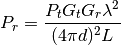
With:
: transmission power (W)
: reception power (W)
: transmission gain (unit-less)
: reception gain (unit-less)
: wavelength (m)
In the implementation, is calculated as
 , where
  m/s is the speed of light in
vacuum, and is the frequency in Hz which can be configured by
the user via the Frequency attribute.
m/s is the speed of light in
vacuum, and is the frequency in Hz which can be configured by
the user via the Frequency attribute.
The Friis model is valid only for propagation in free space within
the so-called far field region, which can be considered
approximately as the region for  .
The model will still return a value for
.
The model will still return a value for  , as
doing so (rather than triggering a fatal error) is practical for
many simulation scenarios. However, we stress that the values
obtained in such conditions shall not be considered realistic.
, as
doing so (rather than triggering a fatal error) is practical for
many simulation scenarios. However, we stress that the values
obtained in such conditions shall not be considered realistic.
Related with this issue, we note that the Friis formula is
undefined for  , and results in
 for
for  .
.
Both these conditions occur outside of the far field region, so in
principle the Friis model shall not be used in these conditions.
In practice, however, Friis is often used in scenarios where accurate
propagation modeling is not deemed important, and values of
can occur.
To allow practical use of the model in such
scenarios, we have to 1) return some value for , and
2) avoid large discontinuities in propagation loss values (which
could lead to artifacts such as bogus capture effects which are
much worse than inaccurate propagation loss values). The two issues
are conflicting, as, according to the Friis formula,
 ;
so if, for , we use a fixed loss value, we end up with an infinitely large
discontinuity, which as we discussed can cause undesirable
simulation artifacts.
;
so if, for , we use a fixed loss value, we end up with an infinitely large
discontinuity, which as we discussed can cause undesirable
simulation artifacts.
To avoid these artifact, this implementation of the Friis model
provides an attribute called MinLoss which allows to specify the
minimum total loss (in dB) returned by the model. This is used in
such a way that
continuously increases for  , until
MinLoss is reached, and then stay constant; this allow to
return a value for and at the same time avoid
discontinuities. The model won’t be much realistic, but at least
the simulation artifacts discussed before are avoided. The default value of
MinLoss is 0 dB, which means that by default the model will return
, until
MinLoss is reached, and then stay constant; this allow to
return a value for and at the same time avoid
discontinuities. The model won’t be much realistic, but at least
the simulation artifacts discussed before are avoided. The default value of
MinLoss is 0 dB, which means that by default the model will return
 for
for 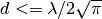 .
We note that this value of is outside of the far field
region, hence the validity of the model in the far field region is
not affected.
.
We note that this value of is outside of the far field
region, hence the validity of the model in the far field region is
not affected.
TwoRayGroundPropagationLossModel
This model implements a Two-Ray Ground propagation loss model ported from NS2
The Two-ray ground reflection model uses the formula
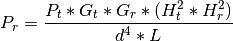
The original equation in Rappaport’s book assumes  .
To be consistent with the free space equation, is added here.
.
To be consistent with the free space equation, is added here.
 and
and  are set at the respective nodes
  coordinate plus a model parameter
set via SetHeightAboveZ.
coordinate plus a model parameter
set via SetHeightAboveZ.
The two-ray model does not give a good result for short distances, due to the oscillation caused by constructive and destructive combination of the two rays. Instead the Friis free-space model is used for small distances.
The crossover distance, below which Friis is used, is calculated as follows:
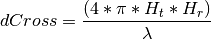
In the implementation, is calculated as
, where m/s is the speed of light in
vacuum, and is the frequency in Hz which can be configured by
the user via the Frequency attribute.
LogDistancePropagationLossModel
This model implements a log distance propagation model.
The reception power is calculated with a so-called log-distance propagation model:
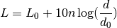
where:
: reference distance (m)
: path loss at reference distance (dB)
When the path loss is requested at a distance smaller than the reference distance, the tx power is returned.
ThreeLogDistancePropagationLossModel
This model implements a log distance path loss propagation model with three distance fields. This model is the same as ns3::LogDistancePropagationLossModel except that it has three distance fields: near, middle and far with different exponents.
Within each field the reception power is calculated using the log-distance propagation equation:
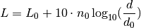
Each field begins where the previous ends and all together form a continuous function.
There are three valid distance fields: near, middle, far. Actually four: the first from 0 to the reference distance is invalid and returns txPowerDbm.

Complete formula for the path loss in dB:
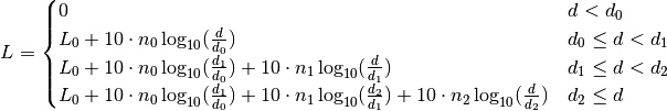
where:
: three distance fields (m)
: path loss distance exponent for each field (unitless)
When the path loss is requested at a distance smaller than the reference
distance , the tx power (with no path loss) is returned. The
reference distance defaults to 1m and reference loss defaults to
FriisPropagationLossModel with 5.15 GHz and is thus = 46.67 dB.
RandomPropagationLossModel
The propagation loss is totally random, and it changes each time the model is called. As a consequence, all the packets (even those between two fixed nodes) experience a random propagation loss.
NakagamiPropagationLossModel
This propagation loss model implements the Nakagami-m fast fading model, which accounts for the variations in signal strength due to multipath fading. The model does not account for the path loss due to the distance traveled by the signal, hence for typical simulation usage it is recommended to consider using it in combination with other models that take into account this aspect.
The Nakagami-m distribution is applied to the power level. The probability density function is defined as
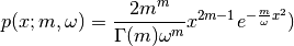
with the fading depth parameter and  the average received power.
It is implemented by either a GammaRandomVariable or a ErlangRandomVariable
random variable.
The implementation of the model allows to specify different values of
the parameter (and hence different fast fading profiles)
for three different distance ranges:

For  the Nakagami-m distribution equals the Rayleigh distribution. Thus
this model also implements Rayleigh distribution based fast fading.
the Nakagami-m distribution equals the Rayleigh distribution. Thus
this model also implements Rayleigh distribution based fast fading.
FixedRssLossModel
This model sets a constant received power level independent of the transmit power.
The received power is constant independent of the transmit power; the user must set received power level. Note that if this loss model is chained to other loss models, it should be the first loss model in the chain. Else it will disregard the losses computed by loss models that precede it in the chain.
MatrixPropagationLossModel
The propagation loss is fixed for each pair of nodes and doesn’t depend on their actual positions. This model should be useful for synthetic tests. Note that by default the propagation loss is assumed to be symmetric.
RangePropagationLossModel
This propagation loss depends only on the distance (range) between transmitter and receiver.
The single MaxRange attribute (units of meters) determines path loss. Receivers at or within MaxRange meters receive the transmission at the transmit power level. Receivers beyond MaxRange receive at power -1000 dBm (effectively zero).
OkumuraHataPropagationLossModel
This model is used to model open area pathloss for long distance (i.e., > 1 Km). In order to include all the possible frequencies usable by LTE we need to consider several variants of the well known Okumura Hata model. In fact, the original Okumura Hata model [hata] is designed for frequencies ranging from 150 MHz to 1500 MHz, the COST231 [cost231] extends it for the frequency range from 1500 MHz to 2000 MHz. Another important aspect is the scenarios considered by the models, in fact the all models are originally designed for urban scenario and then only the standard one and the COST231 are extended to suburban, while only the standard one has been extended to open areas. Therefore, the model cannot cover all scenarios at all frequencies. In the following we detail the models adopted.
The pathloss expression of the COST231 OH is:

where

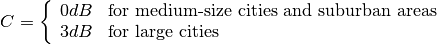
and
: eNB height above the ground [m]
: UE height above the ground [m]
: is a logarithm in base 10 (this for the whole document)
This model is only for urban scenarios.
The pathloss expression of the standard OH in urban area is:

where for small or medium sized city

and for large cities
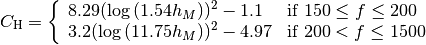
There extension for the standard OH in suburban is
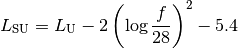
where
: pathloss in urban areas
The extension for the standard OH in open area is

The literature lacks of extensions of the COST231 to open area (for suburban it seems that we can just impose C = 0); therefore we consider it a special case fo the suburban one.
ItuR1411LosPropagationLossModel
This model is designed for Line-of-Sight (LoS) short range outdoor communication in the frequency range 300 MHz to 100 GHz. This model provides an upper and lower bound respectively according to the following formulas
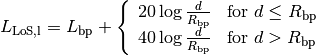
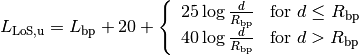
where the breakpoint distance is given by
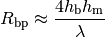
and the above parameters are
: UE height above the ground [m]
and  is the value for the basic transmission loss at the break point, defined as:
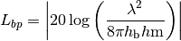
The value used by the simulator is the average one for modeling the median pathloss.
ItuR1411NlosOverRooftopPropagationLossModel
This model is designed for Non-Line-of-Sight (LoS) short range outdoor communication over rooftops in the frequency range 300 MHz to 100 GHz. This model includes several scenario-dependent parameters, such as average street width, orientation, etc. It is advised to set the values of these parameters manually (using the ns-3 attribute system) according to the desired scenario.
In detail, the model is based on [walfisch] and [ikegami], where the loss is expressed
as the sum of free-space loss ( ), the diffraction loss from rooftop to
street (
), the diffraction loss from rooftop to
street ( ) and the reduction due to multiple screen diffraction past
rows of building (
) and the reduction due to multiple screen diffraction past
rows of building ( ). The formula is:
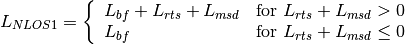
The free-space loss is given by:

where:
The term takes into account the width of the street and its orientation, according to the formulas
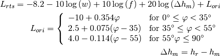
where:
: is the height of the rooftop [m]
: is the height of the mobile [m]
: is the street orientation with respect to the direct path (degrees)
The multiple screen diffraction loss depends on the BS antenna height relative to the building height and on the incidence angle. The former is selected as the higher antenna in the communication link. Regarding the latter, the “settled field distance” is used for select the proper model; its value is given by

with

Therefore, in case of  (where l is the distance over which the building extend),
it can be evaluated according to
(where l is the distance over which the building extend),
it can be evaluated according to
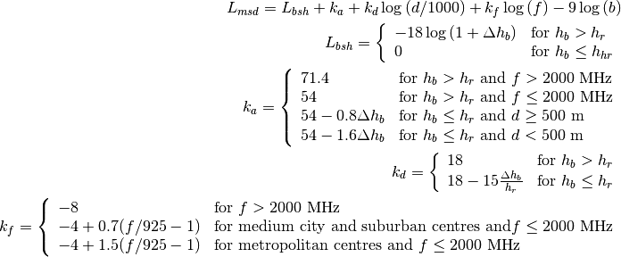
Alternatively, in case of  , the formula is:
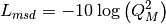
where
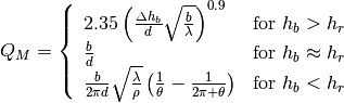
where:
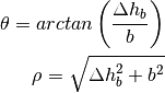
Kun2600MhzPropagationLossModel
This is the empirical model for the pathloss at 2600 MHz for urban areas which is described in [kun2600mhz].
The model is as follows. Let be the distance between the transmitter and the receiver
in meters; the pathloss in dB is calculated as:
ThreeGppPropagationLossModel
The base class ThreeGppPropagationLossModel and its derived classes implement
the path loss and shadow fading models described in 3GPP TR 38.901 [38901].
3GPP TR 38.901 includes multiple scenarios modeling different propagation
environments, i.e., indoor, outdoor urban and rural, for frequencies between
0.5 and 100 GHz.
Implemented features:
- Path loss and shadowing models (3GPP TR 38.901, Sec. 7.4.1)
- Autocorrelation of shadow fading (3GPP TR 38.901, Sec. 7.4.4)
- Channel condition models (3GPP TR 38.901, Sec. 7.4.2)
To be implemented:
- O2I penetration loss (3GPP TR 38.901, Sec. 7.4.3)
- Spatial consistent update of the channel states (3GPP TR 38.901 Sec. 7.6.3.3)
Configuration
The ThreeGppPropagationLossModel instance is paired with a ChannelConditionModel
instance used to retrieve the LOS/NLOS channel condition. By default, a 3GPP
channel condition model related to the same scenario is set (e.g., by default,
ThreeGppRmaPropagationLossModel is paired with
ThreeGppRmaChannelConditionModel), but it can be configured using
the method SetChannelConditionModel. The channel condition models are stored inside the
propagation module, for a limitation of the current spectrum API and to avoid
a circular dependency between the spectrum and the propagation modules. Please
note that it is necessary to install at least one ChannelConditionModel when
using any ThreeGppPropagationLossModel subclass. Please look below for more
information about the Channel Condition models.
The operating frequency has to be set using the attribute “Frequency”, otherwise an assert is raised. The addition of the shadow fading component can be enabled/disabled through the attribute “ShadowingEnabled”. Other scenario-related parameters can be configured through attributes of the derived classes.
Implementation details
The method DoCalcRxPower computes the propagation loss considering the path loss and the shadow fading (if enabled). The path loss is computed by the method GetLossLos or GetLossNlos depending on the LOS/NLOS channel condition, and their implementation is left to the derived classes. The shadow fading is computed by the method GetShadowing, which generates an additional random loss component characterized by Gaussian distribution with zero mean and scenario-specific standard deviation. Subsequent shadowing components of each BS-UT link are correlated as described in 3GPP TR 38.901, Sec. 7.4.4 [38901].
Note 1: The TR defines height ranges for UTs and BSs, depending on the chosen propagation model (for the exact values, please see below in the specific model documentation). If the user does not set correct values, the model will emit a warning but perform the calculation anyway.
Note 2: The 3GPP model is originally intended to be used to represent BS-UT links. However, in ns-3, we may need to compute the pathloss between two BSs or UTs to evaluate the interference. We have decided to support this case by considering the tallest node as a BS and the smallest as a UT. As a consequence, the height values may be outside the validity range of the chosen class: therefore, an inaccuracy warning may be printed, but it can be ignored.
There are four derived class, each one implementing the propagation model for a different scenario:
ThreeGppRMaPropagationLossModel
This class implements the LOS/NLOS path loss and shadow fading models described in 3GPP TR 38.901 [38901], Table 7.4.1-1 for the RMa scenario. It supports frequencies between 0.5 and 30 GHz. It is possible to configure some scenario-related parameters through the attributes AvgBuildingHeight and AvgStreetWidth.
As specified in the TR, the 2D distance between the transmitter and the receiver should be between 10 m and 10 km for the LOS case, or between 10 m and 5 km for the NLOS case, otherwise the model may not be accurate (a warning message is printed if the user has enabled logging on the model). Also, the height of the base station (hBS) should be between 10 m and 150 m, while the height of the user terminal (hUT) should be between 1 m and 10 m.
ThreeGppUMaPropagationLossModel
This implements the LOS/NLOS path loss and shadow fading models described in 3GPP TR 38.901 [38901], Table 7.4.1-1 for the UMa scenario. It supports frequencies between 0.5 and 100 GHz.
As specified in the TR, the 2D distance between the transmitter and the receiver should be between 10 m and 5 km both for the LOS and NLOS cases, otherwise the model may not be accurate (a warning message is printed if the user has enabled logging on the model). Also, the height of the base station (hBS) should be 25 m and the height of the user terminal (hUT) should be between 1.5 m and 22.5 m.
ThreeGppUmiStreetCanyonPropagationLossModel
This implements the LOS/NLOS path loss and shadow fading models described in 3GPP TR 38.901 [38901], Table 7.4.1-1 for the UMi-Street Canyon scenario. It supports frequencies between 0.5 and 100 GHz.
As specified in the TR, the 2D distance between the transmitter and the receiver should be between 10 m and 5 km both for the LOS and NLOS cases, otherwise the model may not be accurate (a warning message is printed if the user has enabled logging on the model). Also, the height of the base station (hBS) should be 10 m and the height of the user terminal (hUT) should be between 1.5 m and 10 m (the validity range is reduced because we assume that the height of the UT nodes is always lower that the height of the BS nodes).
ThreeGppIndoorOfficePropagationLossModel
This implements the LOS/NLOS path loss and shadow fading models described in 3GPP TR 38.901 [38901], Table 7.4.1-1 for the Indoor-Office scenario. It supports frequencies between 0.5 and 100 GHz.
As specified in the TR, the 3D distance between the transmitter and the receiver should be between 1 m and 150 m both for the LOS and NLOS cases, otherwise the model may not be accurate (a warning log message is printed if the user has enabled logging on the model).
Testing
The test suite ThreeGppPropagationLossModelsTestSuite provides test cases for the classes
implementing the 3GPP propagation loss models.
The test cases ThreeGppRmaPropagationLossModelTestCase,
ThreeGppUmaPropagationLossModelTestCase,
ThreeGppUmiPropagationLossModelTestCase and
ThreeGppIndoorOfficePropagationLossModelTestCase compute the path loss between two nodes and compares it with the value obtained using the formulas in 3GPP TR 38.901 [38901], Table 7.4.1-1.
The test case ThreeGppShadowingTestCase checks if the shadowing is correctly computed by testing the deviation of the overall propagation loss from the path loss. The test is carried out for all the scenarios, both in LOS and NLOS condition.
ChannelConditionModel
The loss models require to know if two nodes are in Line-of-Sight (LoS) or if
they are not. The interface for that is represented by this class. The main
method is GetChannelCondition (a, b), which returns a ChannelCondition object
containing the information about the channel state.
We modeled the LoS condition in two ways: (i) by using a probabilistic model specified by the 3GPP (), and (ii) by using an ns-3 specific building-aware model, which checks the space position of the BSs and the UTs. For what regards the first option, the probability is independent of the node location: in other words, following the 3GPP model, two UT spatially separated by an epsilon may have different LoS conditions. To take into account mobility, we have inserted a parameter called “UpdatePeriod,” which indicates how often a 3GPP-based channel condition has to be updated. By default, this attribute is set to 0, meaning that after the channel condition is generated, it is never updated. With this default value, we encourage the users to run multiple simulations with different seeds to get statistical significance from the data. For the users interested in using mobile nodes, we suggest changing this parameter to a value that takes into account the node speed and the desired accuracy. For example, lower-speed node conditions may be updated in terms of seconds, while high-speed UT or BS may be updated more often.
The two approach are coded, respectively, in the classes:
ThreeGppChannelConditionModelBuildingsChannelConditionModel(see thebuildingmodule documentation for further details)
ThreeGppChannelConditionModel
This is the base class for the 3GPP channel condition models. It provides the possibility to updated the condition of each channel periodically, after a given time period which can be configured through the attribute “UpdatePeriod”. If “UpdatePeriod” is set to 0, the channel condition is never updated. It has five derived classes implementing the channel condition models described in 3GPP TR 38.901 [38901] for different propagation scenarios.
ThreeGppRmaChannelConditionModel
This implements the statistical channel condition model described in 3GPP TR 38.901 [38901], Table 7.4.2-1, for the RMa scenario.
ThreeGppUmaChannelConditionModel
This implements the statistical channel condition model described in 3GPP TR 38.901 [38901], Table 7.4.2-1, for the UMa scenario.
ThreeGppUmiStreetCanyonChannelConditionModel
This implements the statistical channel condition model described in 3GPP TR 38.901 [38901], Table 7.4.2-1, for the UMi-Street Canyon scenario.
Testing
The test suite ChannelConditionModelsTestSuite contains a single test case:
ThreeGppChannelConditionModelTestCase, which tests all the 3GPP channel condition models. It determines the channel condition between two nodes multiple times, estimates the LOS probability, and compares it with the value given by the formulas in 3GPP TR 38.901 [38901], Table 7.4.2-1
PropagationDelayModel
The following propagation delay models are implemented:
- ConstantSpeedPropagationDelayModel
- RandomPropagationDelayModel
ConstantSpeedPropagationDelayModel
In this model, the signal travels with constant speed. The delay is calculated according with the transmitter and receiver positions. The Euclidean distance between the Tx and Rx antennas is used. Beware that, according to this model, the Earth is flat.
RandomPropagationDelayModel
The propagation delay is totally random, and it changes each time the model is called. All the packets (even those between two fixed nodes) experience a random delay. As a consequence, the packets order is not preserved.
Models for vehicular environments
The 3GPP TR 37.885 [37885] specifications extends the channel modeling framework described in TR 38.901 [38901] to simulate wireless channels in vehicular environments. The extended framework supports frequencies between 0.5 to 100 GHz and provides the possibility to simulate urban and highway propagation environments. To do so, new propagation loss and channel condition models, as well as new parameters for the fast fading model, are provided.
Vehicular channel condition models
To properly capture channel dynamics in vehicular environments, three different channel conditions have been identified:
- LOS (Line Of Sight): represents the case in which the direct path between the transmitter and the receiver is not blocked
- NLOSv (Non Line Of Sight vehicle): when the direct path between the transmitter and the receiver is blocked by a vehicle
- NLOS (Non Line Of Sight): when the direct path is blocked by a building
TR 37.885 includes two models that can be used to determine the condition of the wireless channel between a pair of nodes, the first for urban and the second for highway environments. Each model includes both a deterministic and a stochastic part, and works as follows:
- The model determines the presence of buildings obstructing the direct path between the communicating nodes. This is done in a deterministic way, looking at the possible interceptions between the direct path and the buildings. If the path is obstructed, the channel condition is set to NLOS.
- If not, the model determines the presence of vehicles obstructing the direct path. This is done using a probabilistic model, which is specific for the scenario of interest. If the path is obstructed, the channel condition is set to NLOSv, otherwise is set to LOS.
These models have been implemented by extending the interface
ChannelConditionModel with the following classes. They have been included in
the building module, because they make use of Buildings objects to determine
the presence of obstructions caused by buildings.
ThreeGppV2vUrbanChannelConditionModel: implements the model described in Table 6.2-1 of TR 37.885 for the urban scenario.ThreeGppV2vHighwayChannelConditionModel: implements the model described in Table 6.2-1 of TR 37.885 for the highway scenario.
These models rely on Buildings objects to determine the presence
of obstructing buildings. When considering large scenarios with a large number of
buildings, this process may become computationally demanding and dramatically
increase the simulation time.
To solve this problem, we implemented two fully-probabilistic models
that can be used as an alternative to the ones included in TR 37.885.
These models are based on the work carried out by M. Boban et al. [Boban2016Modeling],
which derived a statistical representation of the three channel conditions,
With the fully-probabilistic models there is no need to determine the presence of blocking
buildings in a deterministic way, and therefore the computational effort is
reduced.
To determine the channel condition, these models account for the propagation
environment, i.e., urban or highway, as well as for the density of vehicles in the
scenario, which can be high, medium, or low.
The classes implementing the fully-probabilistic models are:
ProbabilisticV2vUrbanChannelConditionModel: implements the model described in [Boban2016Modeling] for the urban scenario.ProbabilisticV2vHighwayChannelConditionModel: implements the model described in [Boban2016Modeling] for the highway scenario.
Both the classes own the attribute “Density”, which can be used to select the
proper value depending on the scenario that have to be simulated.
Differently from the hybrid models described above, these classes have been
included in the propagation module, since they do not have any dependency on the
building module.
NOTE: Both the hybrid and the fully-probabilistic models supports the modeling of outdoor scenarios, no support is provided for the modeling of indoor scenarios.
Vehicular propagation loss models
The propagation models described in TR 37.885 determines the attenuation caused by path loss and shadowing by considering the propagation environment and the channel condition.
These models have been implemented by extending the interface
ThreeGppPropagationLossModel with the following classes, which
are part of the propagation module:
ThreeGppV2vUrbanPropagationLossModel: implements the models defined in Table 6.2.1-1 of TR 37.885 for the urban scenario.ThreeGppV2vHighwayPropagationLossModel: implements the models defined in Table 6.2.1-1 of TR 37.885 for the highway scenario.
As for all the classes extending the interface ThreeGppPropagationLossModel,
they have to be paired with an instance of the class ChannelConditionModel
which is used to determine the channel condition.
This is done by setting the attribute ChannelConditionModel.
To build the channel modeling framework described in TR 37.885,
ThreeGppV2vUrbanChannelConditionModel or
ThreeGppV2vHighwayChannelConditionModel should be used, but users
are allowed to test any other combination.
Vehicular fast fading model
The fast fading model described in Sec. 6.2.3 of TR 37.885 is based on the one
specified in TR 38.901, whose implementation is provided in the spectrum module
(see the spectrum module documentation).
This model is general and includes different parameters which can
be tuned to simulate multiple propagation environments.
To better model the channel dynamics in vehicular environments, TR 37.885
provides new sets of values for these parameters, specific for
vehicle-to-vehicle transmissions in urban and highway scenarios.
To select the parameters for vehicular scenarios, it is necessary to set
the attribute “Scenario” of the class ThreeGppChannelModel using the value
“V2V-Urban” or “V2V-Highway”.
Additionally, TR 37.885 specifies a new equation to compute the Doppler component,
which accounts for the mobility of both nodes, as well as scattering
from the environment.
In particular, the scattering effect is considered by deviating the Doppler
frequency by a random value, whose distribution depends on the parameter  .
TR 37.885 specifies that should be set to the maximum speed of the
vehicles in the layout and, if
.
TR 37.885 specifies that should be set to the maximum speed of the
vehicles in the layout and, if  , the scattering effect is not considered.
The Doppler equation is implemented in the class
, the scattering effect is not considered.
The Doppler equation is implemented in the class ThreeGppSpectrumPropagationLossModel.
By means of the attribute “vScatt”, it is possible to adjust the value of
(by default, the value is set to 0).
Example
We implemented the example three-gpp-v2v-channel-example.cc which shows how to
configure the different classes to simulate wireless propagation in vehicular
scenarios, it can be found in the folder examples/channel-models.
We considered two communicating vehicles moving within the scenario, and computed the SNR experienced during the entire simulation, with a time resolution of 10 ms. The vehicles are equipped with 2x2 antenna arrays modeled using the 3GPP antenna model. The bearing and the downtilt angles are properly configured and the optimal beamforming vectors are computed at the beginning of the simulation.
The simulation script accepts the following command line parameters:
- frequency: the operating frequency in Hz
- txPow: the transmission power in dBm
- noiseFigure: the noise figure in dB
- scenario: the simulation scenario, “V2V-Urban” or “V2V-Highway”
The “V2V-Urban” scenario simulates urban environment with a rectangular grid of buildings. The vehicles moves with a waypoint mobility model. They start from the same position and travel in the same direction, along the main street. The first vehicle moves at 60 km/h and the second at 30 km/h. At a certain point, the first vehicle turns left while the second continues on the main street.
The “V2V-Highway” scenario simulates an highway environment in which the two vehicles travel on the same lane, in the same direction, and keep a safety distance of 20 m. They maintain a constant speed of 140 km/h.
The example generates the output file example-output.txt. Each row of the
file is organized as follows:
Time[s] TxPosX[m] TxPosY[m] RxPosX[m] RxPosY[m] ChannelState SNR[dB] Pathloss[dB]
We also provide the bash script three-gpp-v2v-channel-example.sh which reads the
output file and generates two figures:
- map.gif, a GIF representing the simulation scenario and vehicle mobility;
- snr.png, which represents the behavior of the SNR.
References
| [friis] | Friis, H.T., “A Note on a Simple Transmission Formula,” Proceedings of the IRE , vol.34, no.5, pp.254,256, May 1946 |
| [hata] | M.Hata, “Empirical formula for propagation loss in land mobile radio services”, IEEE Trans. on Vehicular Technology, vol. 29, pp. 317-325, 1980 |
| [cost231] | “Digital Mobile Radio: COST 231 View on the Evolution Towards 3rd Generation Systems”, Commission of the European Communities, L-2920, Luxembourg, 1989 |
| [walfisch] | J.Walfisch and H.L. Bertoni, “A Theoretical model of UHF propagation in urban environments,” in IEEE Trans. Antennas Propagat., vol.36, 1988, pp.1788- 1796 |
| [ikegami] | F.Ikegami, T.Takeuchi, and S.Yoshida, “Theoretical prediction of mean field strength for Urban Mobile Radio”, in IEEE Trans. Antennas Propagat., Vol.39, No.3, 1991 |
| [kun2600mhz] | Sun Kun, Wang Ping, Li Yingze, “Path loss models for suburban scenario at 2.3GHz, 2.6GHz and 3.5GHz”, in Proc. of the 8th International Symposium on Antennas, Propagation and EM Theory (ISAPE), Kunming, China, Nov 2008. |
| [38901] | (1, 2, 3, 4, 5, 6, 7, 8, 9, 10, 11, 12, 13, 14, 15) 3GPP. 2018. TR 38.901, Study on channel model for frequencies from 0.5 to 100 GHz, V15.0.0. (2018-06). |
| [37885] | 3GPP. 2019. TR 37.885, Study on evaluation methodology of new Vehicle-to-Everything (V2X) use cases for LTE and NR, V15.3.0. (2019-06). |
| [Boban2016Modeling] | (1, 2, 3) M. Boban, X. Gong, and W. Xu, “Modeling the evolution of line-of-sight blockage for V2V channels,” in IEEE 84th Vehicular Technology Conference (VTC-Fall), 2016. |
Spectrum Module
The Spectrum module aims at providing support for modeling the frequency-dependent aspects of communications in ns-3. The model was first introduced in [Baldo2009Spectrum], and has been enhanced and refined over the years.
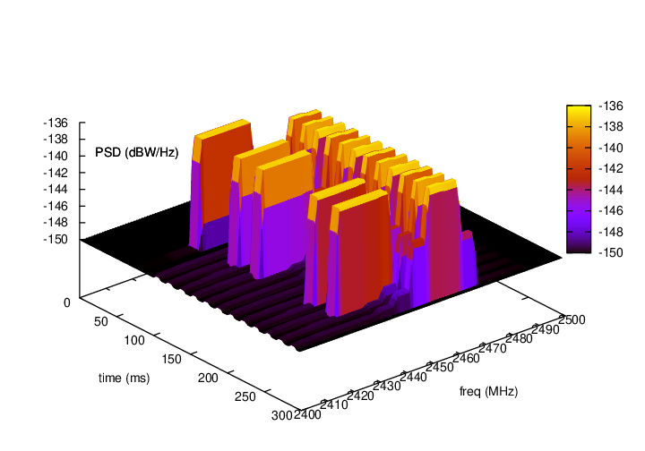
Spectrogram produced by a spectrum analyzer in a scenario
involving wifi signals interfered by a microwave oven, as simulated
by the example adhoc-aloha-ideal-phy-with-microwave-oven.
Model Description
The module provides:
- a set of classes for modeling signals and
- a Channel/PHY interface based on a power spectral density signal representation that is technology-independent
- two technology-independent Channel implementations based on the Channel/PHY interface
- a set of basic PHY model implementations based on the Channel/PHY interface
The source code for the spectrum module is located at src/spectrum.
Design
Signal model
The signal model is implemented by the
SpectrumSignalParameters class. This class provides the following
information for a signal being transmitted/received by PHY devices:
- a reference to the transmitting PHY device
- a reference to the antenna model used by the transmitting PHY device to transmit this signal
- the duration of the signal
- its Power Spectral Density (PSD) of the signal, which is assumed to be constant for the duration of the signal.
The PSD is represented as a set of discrete scalar values each
corresponding to a certain subband in frequency. The set of frequency subbands
to which the PSD refers to is defined by an instance of the
SpectrumModel class. The PSD itself is implemented as an instance
of the SpectrumValue class which contains a reference to the
associated SpectrumModel class instance. The SpectrumValue
class provides several arithmetic operators to allow to perform calculations
with PSD instances. Additionally, the SpectrumConverter class
provides means for the conversion of SpectrumValue instances from
one SpectrumModel to another.
For a more formal mathematical description of the signal model just described, the reader is referred to [Baldo2009Spectrum].
The SpectrumSignalParameters class is meant to include only
information that is valid for all signals; as such, it is not meant to
be modified to add technology-specific information (such as type of
modulation and coding schemes used, info on preambles and reference
signals, etc). Instead, such information shall be put in a new class
that inherits from SpectrumSignalParameters and extends it with
any technology-specific information that is needed. This design
is intended to model the fact that in the real world we have signals
of different technologies being simultaneously transmitted and
received over the air.
Channel/PHY interface
The spectrum Channel/PHY interface is defined by the base classes SpectrumChannel
and SpectrumPhy. Their interaction simulates the transmission and
reception of signals over the medium. The way this interaction works is depicted in Sequence diagram showing the interaction between SpectrumPhy and SpectrumChannel:
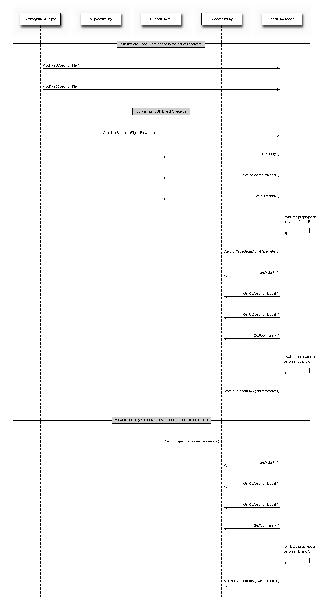
Sequence diagram showing the interaction between SpectrumPhy and SpectrumChannel
Spectrum Channel implementations
The module provides two SpectrumChannel implementations:
SingleModelSpectrumChannel and MultiModelSpectrumChannel. They
both provide this functionality:
- Propagation loss modeling, in two forms:
- you can plug models based on
PropagationLossModelon these channels. Only linear models (where the loss value does not depend on the transmission power) can be used. These models are single-frequency in the sense that the loss value is applied equally to all components of the power spectral density.- you can plug models based on
SpectrumPropagationLossModelon these channels. These models can have frequency-dependent loss, i.e., a separate loss value is calculated and applied to each component of the power spectral density.- Propagation delay modeling, by plugging a model based on
PropagationDelayModel. The delay is independent of frequency and applied to the signal as a whole. Delay modeling is implemented by scheduling theStartRxevent with a delay respect to theStartTxevent.
SingleModelSpectrumChannel and MultiModelSpectrumChannel are
quite similar, the main difference is that
MultiModelSpectrumChannel allows to use different
SpectrumModel instances with the same channel instance, by
automatically taking care of the conversion of PSDs among the
different models.
Example model implementations
The spectrum module provides some basic implementation of several components that are mainly intended as a proof-of-concept and as an example for building custom models with the spectrum module. Here is a brief list of the available implementations:
SpectrumModel300Khz300GhzLogandSpectrumModelIsm2400MhzRes1Mhzare two exampleSpectrumModelimplementationsHalfDuplexIdealPhy: a basic PHY model using a gaussian interference model (implemented inSpectrumInterference) together with an error model based on Shannon capacity (described in [Baldo2009Spectrum] and implemented inSpectrumErrorModel. This PHY uses theGenericPhyinterface. Its addditional custom signal parameters are defined inHalfDuplexIdealPhySignalParameters.WifiSpectrumValueHelperis an helper object that makes it easy to createSpectrumValuesrepresenting PSDs and RF filters for the wifi technology.AlohaNoackNetDevice: a minimal NetDevice that allows to send packets overHalfDuplexIdealPhy(or other PHY model based on theGenericPhyinterface).SpectrumAnalyzer,WaveformGeneratorandMicrowaveOvenare examples of PHY models other than communication devices - the names should be self-explaining.
Usage
The main use case of the spectrum model is for developers who want to develop a new model for the PHY layer of some wireless technology to be used within ns-3. Here are some notes on how the spectrum module is expected to be used.
SpectrumPhyandSpectrumChannelare abstract base classes. Real code will use classes that inherit from these classes.If you are implementing a new model for some wireless technology of your interest, and want to use the spectrum module, you’ll typically create your own module and make it depend on the spectrum module. Then you typically have to implement:
- a child class of
SpectrumModelwhich defines the (sets of) frequency subbands used by the considered wireless technology. Note: instances ofSpectrumModelare typically statically allocated, in order to allow severalSpectrumValueinstances to reference the sameSpectrumModelinstance.- a child class of
SpectrumPhywhich will handle transmission and reception of signals (including, if appropriate, interference and error modeling).- a child class of
SpectrumSignalParameterswhich will contain all the information needed to model the signals for the wireless technology being considered that is not already provided by the baseSpectrumSignalParametersclass. Examples of such information are the type of modulation and coding schemes used, the PHY preamble format, info on the pilot/reference signals, etc.The available
SpectrumChannelimplementations (SingleModelSpectrumChannelandMultiModelSpectrumChannel, are quite generic. Chances are you can use them as-is. Whether you prefer one or the other it is just a matter of whether you will have a single SpectrumModel or multiple ones in your simulations.Typically, there will be a single SpectrumChannel instance to which several SpectrumPhy instances are plugged. The rule of thumb is that all PHYs that are interfering with each other shall be plugged on the same channel. Multiple SpectrumChannel instances are expected to be used mainly when simulating completely orthogonal channels; for example, when simulating the uplink and downlink of a Frequency Division Duplex system, it is a good choice to use two SpectrumChannel instances in order to reduce computational complexity.
Different types of SpectrumPhy (i.e., instances of different child classes) can be plugged on the same SpectrumChannel instance. This is one of the main features of the spectrum module, to support inter-technology interference. For example, if you implement a WifiSpectrumPhy and a BluetoohSpectrumPhy, and plug both on a SpectrumChannel, then you’ll be able to simulate interference between wifi and bluetooth and vice versa.
Different child classes of
SpectrumSignalParameterscan coexist in the same simulation, and be transmitted over the same channel object. Again, this is part of the support for inter-technology interference. A PHY device model is expected to use theDynamicCast<>operator to determine if a signal is of a certain type it can attempt to receive. If not, the signal is normally expected to be considered as interference.
Helpers
The helpers provided in src/spectrum/helpers are mainly intended
for the example implementations described in Example model implementations.
If you are developing your custom model based on the
spectrum framework, you will probably prefer to define your own
helpers.
Attributes
- Both
SingleModelSpectrumChannelandMultiModelSpectrumChannelhave an attributeMaxLossDbwhich can use to avoid propagating signals affected by very high propagation loss. You can use this to reduce the complexity of interference calculations. Just be careful to choose a value that does not make the interference calculations inaccurate.- The example implementations described in Example model implementations also have several attributes.
Output
- Both
SingleModelSpectrumChannelandMultiModelSpectrumChannelprovide a trace source calledPathLosswhich is fired whenever a new path loss value is calclulated. Note: only single-frequency path loss is accounted for, see the attribute description.- The example implementations described in Example model implementations also provide some trace sources.
- The helper class
SpectrumAnalyzerHelpercan be conveniently used to generate an output text file containing the spectrogram produced by a SpectrumAnalyzer instance. The format is designed to be easily plotted withgnuplot. For example, if your run the exampleadhoc-aloha-ideal-phy-with-microwave-ovenyou will get an output file calledspectrum-analyzer-output-3-0.tr. From this output file, you can generate a figure similar to Spectrogram produced by a spectrum analyzer in a scenario involving wifi signals interfered by a microwave oven, as simulated by the example adhoc-aloha-ideal-phy-with-microwave-oven. by executing the following gnuplot commands:
unset surface
set pm3d at s
set palette
set key off
set view 50,50
set xlabel "time (ms)"
set ylabel "freq (MHz)"
set zlabel "PSD (dBW/Hz)" offset 15,0,0
splot "./spectrum-analyzer-output-3-0.tr" using ($1*1000.0):($2/1e6):(10*log10($3))
Examples
The example programs in src/spectrum/examples/ allow to see the
example implementations described in Example model implementations in action.
Troubleshooting
- Disclaimer on inter-technology interference: the spectrum model makes it very easy to implement an inter-technology interference model, but this does not guarantee that the resulting model is accurate. For example, the gaussian interference model implemented in the
SpectrumInterferenceclass can be used to calculate inter-technology interference, however the results might not be valid in some scenarios, depending on the actual waveforms involved, the number of interferers, etc. Moreover, it is very important to use error models that are consistent with the interference model. The responsibility of ensuring that the models being used are correct is left to the user.
Testing
In this section we describe the test suites that are provided within the spectrum module.
SpectrumValue test
The test suite spectrum-value verifies the correct functionality of the arithmetic
operators implemented by the SpectrumValue class. Each test case
corresponds to a different operator. The test passes if the result
provided by the operator implementation is equal to the reference
values which were calculated offline by hand. Equality is verified
within a tolerance of which is to account for
numerical errors.
SpectrumConverter test
The test suite spectrum-converter verifies the correct
functionality of the SpectrumConverter class. Different test cases
correspond to the conversion of different SpectrumValue instances
to different SpectrumModel instances. Each test passes if the
SpectrumValue instance resulting from the conversion is equal to the reference
values which were calculated offline by hand. Equality is verified
within a tolerance of which is to account for
numerical errors.
Describe how the model has been tested/validated. What tests run in the test suite? How much API and code is covered by the tests? Again, references to outside published work may help here.
Interference test
The test suite spectrum-interference verifies the correct
functionality of the SpectrumInterference and
ShannonSpectrumErrorModel in a scenario involving four
signals (an intended signal plus three interferers). Different test
cases are created corresponding to different PSDs of the intended
signal and different amount of transmitted bytes. The test passes if
the output of the error model (successful or failed) coincides with
the expected one which was determine offline by manually calculating
the achievable rate using Shannon’s formula.
IdealPhy test
The test verifies that AlohaNoackNetDevice and
HalfDuplexIdealPhy work properly when installed in a node. The
test recreates a scenario with two nodes (a TX and a RX) affected by a path loss such
that a certain SNR is obtained. The TX node transmits with a
pre-determined PHY rate and with an application layer rate which is
larger than the PHY rate, so as to saturate the
channel. PacketSocket is used in order to avoid protocol
overhead. Different
test cases correspond to different PHY rate and SNR values. For each
test case, we calculated offline (using Shannon’s formula) whether
the PHY rate is achievable or not. Each test case passes if the
following conditions are satisfied:
- if the PHY rate is achievable, the application throughput shall be within
of the PHY rate;
- if the PHY rate is not achievable, the application throughput shall be zero.
Additional Models
TV Transmitter Model
A TV Transmitter model is implemented by the TvSpectrumTransmitter class.
This model enables transmission of realistic TV signals to be simulated and can
be used for interference modeling. It provides a customizable power spectral
density (PSD) model, with configurable attributes including the type of
modulation (with models for analog, 8-VSB, and COFDM), signal bandwidth,
power spectral density level, frequency, and transmission duration. A helper
class, TvSpectrumTransmitterHelper, is also provided to assist users in
setting up simulations.
Main Model Class
The main TV Transmitter model class, TvSpectrumTransmitter, provides a
user-configurable PSD model that can be transmitted on the SpectrumChannel.
It inherits from SpectrumPhy and is comprised of attributes and methods to
create and transmit the signal on the channel.
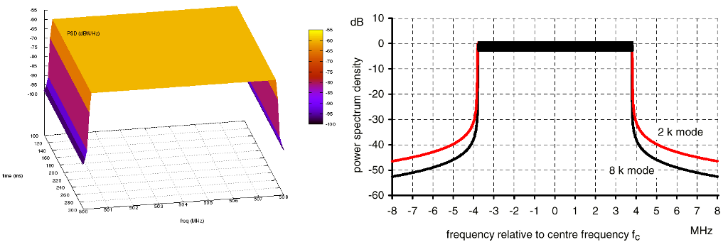
8K COFDM signal spectrum generated from TvSpectrumTransmitter (Left) and
theoretical COFDM signal spectrum [KoppCOFDM] (Right)
One of the user-configurable attributes is the type of modulation for the TV transmitter to use. The options are 8-VSB (Eight-Level Vestigial Sideband Modulation) which is notably used in the North America ATSC digital television standard, COFDM (Coded Orthogonal Frequency Division Multiplexing) which is notably used in the DVB-T and ISDB-T digital television standards adopted by various countries around the world, and analog modulation which is a legacy technology but is still being used by some countries today. To accomplish realistic PSD models for these modulation types, the signals’ PSDs were approximated from real standards and developed into models that are scalable by frequency and power. The COFDM PSD is approximated from Figure 12 (8k mode) of [KoppCOFDM], the 8-VSB PSD is approximated from Figure 3 of [Baron8VSB], and the analog PSD is approximated from Figure 4 of [QualcommAnalog]. Note that the analog model is approximated from the NTSC standard, but other analog modulation standards such as PAL have similar signals. The approximated COFDM PSD model is in 8K mode. The other configurable attributes are the start frequency, signal/channel bandwidth, base PSD, antenna type, starting time, and transmit duration.
TvSpectrumTransmitter uses IsotropicAntennaModel as its antenna model by
default, but any model that inherits from AntennaModel is selectable, so
directional antenna models can also be used. The propagation loss models used
in simulation are configured in the SpectrumChannel that the user chooses to
use. Terrain and spherical Earth/horizon effects may be supported in future ns-3
propagation loss models.
After the attributes are set, along with the SpectrumChannel,
MobilityModel, and node locations, the PSD of the TV transmitter signal can
be created and transmitted on the channel.
Helper Class
The helper class, TvSpectrumTransmitterHelper, consists of features to
assist users in setting up TV transmitters for their simulations. Functionality
is also provided to easily simulate real-world scenarios.
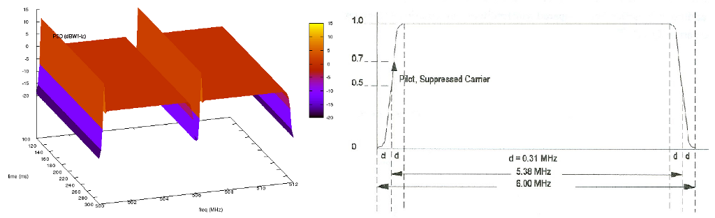
North America ATSC channel 19 & 20 signals generated using
TvSpectrumTransmitterHelper (Left) and theoretical 8-VSB signal
[Baron8VSB] (Right). Note that the theoretical signal is not shown in dB
while the ns-3 generated signals are.
Using this helper class, users can easily set up TV transmitters right after configuring attributes. Multiple transmitters can be created at a time. Also included are real characteristics of specific geographic regions that can be used to run realistic simulations. The regions currently included are North America, Europe, and Japan. The frequencies and bandwidth of each TV channel for each these regions are provided.
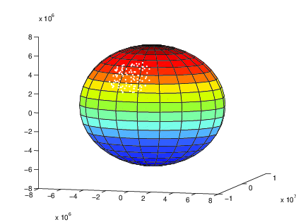
Plot from MATLAB implementation of CreateRegionalTvTransmitters method in
TvSpectrumTransmitterHelper. Shows 100 random points on Earth’s surface
(with altitude 0) corresponding to TV transmitter locations within a 2000 km
radius of 35° latitude and -100° longitude.
A method (CreateRegionalTvTransmitters) is provided that enables users to randomly generate multiple TV transmitters from a specified region with a given density within a chosen radius around a point on Earth’s surface. The region, which determines the channel frequencies of the generated TV transmitters, can be specified to be one of the three provided, while the density determines the amount of transmitters generated. The TV transmitters’ antenna heights (altitude) above Earth’s surface can also be randomly generated to be within a given maximum altitude. This method models Earth as a perfect sphere, and generated location points are referenced accordingly in Earth-Centered Earth-Fixed Cartesian coordinates. Note that bodies of water on Earth are not considered in location point generation–TV transmitters can be generated anywhere on Earth around the origin point within the chosen maximum radius.
Examples
Two example simulations are provided that demonstrate the functionality of the
TV transmitter model. tv-trans-example simulates two 8-VSB TV transmitters
with adjacent channel frequencies. tv-trans-regional-example simulates
randomly generated COFDM TV transmitters (modeling the DVB-T standard)
located around the Paris, France area with channel frequencies and bandwidths
corresponding to the European television channel allocations.
Testing
The tv-spectrum-transmitter test suite verifies the accuracy of the
spectrum/PSD model in TvSpectrumTransmitter by testing if the maximum power
spectral density, start frequency, and end frequency comply with expected values
for various test cases.
The tv-helper-distribution test suite verifies the functionality of the
method in TvSpectrumTransmitterHelper that generates a random number of TV
transmitters based on the given density (low, medium, or high) and maximum
number of TV channels. It verifies that the number of TV transmitters generated
does not exceed the expected bounds.
The CreateRegionalTvTransmitters method in TvSpectrumTransmitterHelper
described in Helper Class uses two methods from the
GeographicPositions class in the Mobility module to generate the random
Cartesian points on or above earth’s surface around an origin point which
correspond to TV transmitter positions. The first method converts Earth
geographic coordinates to Earth-Centered Earth-Fixed (ECEF) Cartesian
coordinates, and is tested in the geo-to-cartesian test suite by comparing
(with 10 meter tolerance) its output with the output of the geographic to ECEF
conversion function [MatlabGeo] of the MATLAB Mapping Toolbox for numerous
test cases. The other used method generates random ECEF Cartesian points around
the given geographic origin point, and is tested in the rand-cart-around-geo
test suite by verifying that the generated points do not exceed the given
maximum distance radius from the origin point.
3GPP TR 38.901 fast fading model
The framework described by TR 38.901 [TR38901] is a 3D statistical Spatial
Channel Model supporting different propagation environments (e.g., urban,
rural, indoor), multi-antenna operations and the modeling of wireless channels
between 0.5 and 100 GHz.
The overall channel is represented by the matrix  , in which each
entry H u,s
, in which each
entry H u,s  corresponds to the impulse response of the channel between the
s-th element of the transmitting antenna and the u-th element of the receiving
antenna. H u,s is generated by the superposition of N different multi-path
components, called clusters, each of which composed of M different rays.
The channel matrix generation procedure accounts for large and small scale
propagation phenomena. The classes ThreeGppSpectrumPropagationLossModel and
ThreeGppChannelModel included in the spectrum module takes care of the generation
of the channel coefficients and the computation of the frequency-dependent
propagation loss.
corresponds to the impulse response of the channel between the
s-th element of the transmitting antenna and the u-th element of the receiving
antenna. H u,s is generated by the superposition of N different multi-path
components, called clusters, each of which composed of M different rays.
The channel matrix generation procedure accounts for large and small scale
propagation phenomena. The classes ThreeGppSpectrumPropagationLossModel and
ThreeGppChannelModel included in the spectrum module takes care of the generation
of the channel coefficients and the computation of the frequency-dependent
propagation loss.
Implementation
Our implementation is described in [Zugno]. It is based on the model described in [Zhang], but the code has been refactored, extended, and aligned to TR 38.901 [TR38901]. The fundamental assumption behind this model is the channel reciprocity, i.e., the impulse response of the channel between node a and node b is the same as between node b and node a. To deal with the equivalence of the channel between a and b, no matter who is the transmitter and who is the receiver, the model considers the pair of nodes to be composed by one “s” and one “u” node. The channel matrix, as well as other parameters, are saved and used under the assumption that, within a pair, the definition of the “s” and “u” node will always be the same. For more details, please have a look at the documentation of the classes ThreeGppChannelModel and ThreeGppSpectrumPropagationLossModel.
Note:
Currently, no error model is provided; a link-to-system campaign may be needed to incorporate it in existing modules.
The model does not include any spatial consistency update procedure (see [TR38901], Sec. 7.6.1). The implementation of this feature is left as future work.
Issue regarding the blockage model: according to 3GPP TR 38.901 v15.0.0 (2018-06) section 7.6.4.1, the blocking region for self-blocking is provided in LCS.
However, here, clusterAOA and clusterZOA are in GCS and blocking check is performed for self-blocking similar to non-self blocking, that is in GCS. One would expect the angles to be transposed to LCS before checking self-blockage.
ThreeGppSpectrumPropagationLossModel
The class ThreeGppSpectrumPropagationLossModel extends the SpectrumPropagationLossModel interface and enables the modeling of frequency dependent propagation phenomena. The main method is DoCalcRxPowerSpectralDensity, which takes as input the power spectral density (PSD) of the transmitted signal, the mobility models of the transmitting node and receiving node, and returns the PSD of the received signal.
Procedure used to compute the PSD of to compute the PSD of the received signal:
1. Retrieve the beamforming vectors To account for the beamforming, ThreeGppSpectrumPropagationLossModel has to retrieve the beamforming vectors of the transmitting and receiving antennas. The method DoCalcRxPowerSpectralDensity uses m_deviceAntennaMap to obtain the antenna objects associated to the transmitting and receiving devices, and calls the method GetCurrentBeamformingVector to retrieve the beamforming vectors. For each device using the channel, the m_deviceAntennaMap contains the associated antenna object of type PhasedArrayModel. Since the mapping is one-to-one, the model supports a single antenna object for each device. The m_deviceAntennaMap has to be initialized by inserting the device-antenna pairs using the method AddDevice.
2. Retrieve the channel matrix The ThreeGppSpectrumPropagationLossModel relies on the ThreeGppChannelModel class to obtain the channel matrix. In particular, it makes use of the method GetChannel, which returns a ChannelMatrix object containing the channel matrix and other channel parameters. The ThreeGppChannelModel instance is automatically created in the the ThreeGppSpectrumPropagationLossModel constructor and it can be configured using the method SetChannelModelAttribute ().
4. Compute the long term component The method GetLongTerm returns the long term component obtained by multiplying the channel matrix and the beamforming vectors. To reduce the computational load, the long term components associated to the different channels are stored in the m_longTermMap and recomputed only if the associated channel matrix is updated or if the transmitting and/or receiving beamforming vectors have changed. Given the channel reciprocity assumption, for each node pair a single long term component is saved in the map.
5. Apply the small scale fading and compute the channel gain
The method CalcBeamformingGain computes the channel gain in each sub-band and
applies it to the PSD of the transmitted signal to obtain the received PSD.
To compute the sub-band gain, it accounts for the Doppler phenomenon and the
time dispersion effect on each cluster.
In order to reduce the computational load, the Doppler component of each
cluster is computed considering only the central ray.
Also, as specified here, it is possible to account for
the effect of environmental scattering following the model described in Sec. 6.2.3
of 3GPP TR 37.885.
This is done by deviating the Doppler frequency by a random value, whose
distribution depends on the parameter .
The value of can be configured using the attribute “vScatt”
(by default it is set to 0, so that the scattering effect is not considered).
ThreeGppChannelModel
The class ThreeGppChannelModel implements the channel matrix generation procedure described in Sec. of [TR38901]. The main method is GetChannel, which takes as input the mobility models of the transmitter and receiver nodes, the associated antenna objects, and returns a ChannelMatrix object containing:
- the channel matrix of size UxSxN, where U is the number of receiving antenna elements, S is the number of transmitting antenna elements and N is the number of clusters
- the clusters delays, as an array of size N
- the clusters arrival and departure angles, as a 2D array in which each row corresponds to a direction (AOA, ZOA, AOD, ZOD) and each column corresponds to a different cluster
- a time stamp indicating the time at which the channel matrix was generated
- the node IDs
- other channel parameters
The ChannelMatrix objects are saved in the map m_channelMap and updated when the coherence time expires, or in case the LOS/NLOS channel condition changes. The coherence time can be configured through the attribute “UpdatePeriod”, and should be chosen by taking into account all the factors that affects the channel variability, such as mobility, frequency, propagation scenario, etc. By default, it is set to 0, which means that the channel is recomputed only when the LOS/NLOS condition changes. It is possible to configure the propagation scenario and the operating frequency of interest through the attributes “Scenario” and “Frequency”, respectively.
Blockage model: 3GPP TR 38.901 also provides an optional feature that can be used to model the blockage effect due to the presence of obstacles, such as trees, cars or humans, at the level of a single cluster. This differs from a complete blockage, which would result in an LOS to NLOS transition. Therefore, when this feature is enabled, an additional attenuation is added to certain clusters, depending on their angle of arrival. There are two possi- ble methods for the computation of the additional attenuation, i.e., stochastic (Model A) and geometric (Model B). In this work, we used the implementation provided by [Zhang], which uses the stochastic method. In particular, the model is implemented by the method CalcAttenuationOfBlockage, which computes the additional attenuation. The blockage feature can be disable through the attribute “Blockage”. Also, the attributes “NumNonselfBlocking”, “PortraitMode” and “BlockerSpeed” can be used to configure the model.
Testing
The test suite ThreeGppChannelTestSuite includes three test cases:
ThreeGppChannelMatrixComputationTest checks if the channel matrix has the correct dimensions and if it correctly normalized
ThreeGppChannelMatrixUpdateTest, which checks if the channel matrix is correctly updated when the coherence time exceeds
ThreeGppSpectrumPropagationLossModelTest, which tests the functionalities of the class ThreeGppSpectrumPropagationLossModel. It builds a simple network composed of two nodes, computes the power spectral density received by the receiving node, and
- Checks if the long term components for the direct and the reverse link are the same,
- Checks if the long term component is updated when changing the beamforming vectors,
- Checks if the long term is updated when changing the channel matrix
Note: TR 38.901 includes a calibration procedure that can be used to validate the model, but it requires some additional features which are not currently implemented, thus is left as future work.
References
| [Baron8VSB] | (1, 2) Baron, Stanley. “First-Hand:Digital Television: The Digital Terrestrial Television Broadcasting (DTTB) Standard.” IEEE Global History Network. <http://www.ieeeghn.org/wiki/index.php/First-Hand:Digital_Television:_The_Digital_Terrestrial_Television_Broadcasting_(DTTB)_Standard>. |
| [KoppCOFDM] | (1, 2) Kopp, Carlo. “High Definition Television.” High Definition Television. Air Power Australia. <http://www.ausairpower.net/AC-1100.html>. |
| [MatlabGeo] | “Geodetic2ecef.” Convert Geodetic to Geocentric (ECEF) Coordinates. The MathWorks, Inc. <http://www.mathworks.com/help/map/ref/geodetic2ecef.html>. |
| [QualcommAnalog] | Stephen Shellhammer, Ahmed Sadek, and Wenyi Zhang. “Technical Challenges for Cognitive Radio in the TV White Space Spectrum.” Qualcomm Incorporated. |
| [TR38901] | (1, 2, 3, 4) 3GPP. 2018. TR 38.901. Study on channel for frequencies from 0.5 to 100 GHz. V.15.0.0. (2018-06). |
| [Zhang] | (1, 2) Menglei Zhang, Michele Polese, Marco Mezzavilla, Sundeep Rangan, Michele Zorzi. “ns-3 Implementation of the 3GPP MIMO Channel Model for Frequency Spectrum above 6 GHz”. In Proceedings of the Workshop on ns-3 (WNS3 ‘17). 2017. |
| [Zugno] | Tommaso Zugno, Michele Polese, Natale Patriciello, Biljana Bojovic, Sandra Lagen, Michele Zorzi. “Implementation of a Spatial Channel Model for ns-3”. Submitted to the Workshop on ns-3 (WNS3 ‘20). 2020. Available: https://arxiv.org/abs/2002.09341 |
6LoWPAN: Transmission of IPv6 Packets over IEEE 802.15.4 Networks
This chapter describes the implementation of ns-3 model for the compression of IPv6 packets over IEEE 802.15.4-Based Networks as specified by RFC 4944 (“Transmission of IPv6 Packets over IEEE 802.15.4 Networks”) and RFC 6282 (“Compression Format for IPv6 Datagrams over IEEE 802.15.4-Based Networks”).
Model Description
The source code for the sixlowpan module lives in the directory src/sixlowpan.
Design
The model design does not follow strictly the standard from an architectural standpoint, as it does extend it beyond the original scope by supporting also other kinds of networks.
Other than that, the module strictly follows RFC 4944 and RFC 6282, with the exception that HC2 encoding is not supported, as it has been superseded by IPHC and NHC compression type (RFC 6282).
IPHC sateful (context-based) compression is supported but, since RFC 6775 (“Neighbor Discovery Optimization for IPv6 over Low-Power Wireless Personal Area Networks (6LoWPANs)”) is not yet implemented, it is necessary to add the context to the nodes manually.
This is possible though the SixLowPanHelper::AddContext function.
Mind that installing different contexts in different nodes will lead to decompression failures.
NetDevice
The whole module is developed as a transparent NetDevice, which can act as a proxy between IPv6 and any NetDevice (the module has been successfully tested with PointToPointNedevice, CsmaNetDevice and LrWpanNetDevice).
For this reason, the module implements a virtual NetDevice, and all the calls are passed without modifications to the underlying NetDevice. The only important difference is in GetMtu behaviour. It will always return at least 1280 bytes, as is the minimum IPv6 MTU.
The module does provide some attributes and some tracesources. The attributes are:
- Rfc6282 (boolean, default true), used to activate HC1 (RFC 4944) or IPHC (RFC 6282) compression.
- OmitUdpChecksum (boolean, default true), used to activate UDP checksum compression in IPHC.
- FragmentReassemblyListSize (integer, default 0), indicating the number of packets that can be reassembled at the same time. If the limit is reached, the oldest packet is discarded. Zero means infinite.
- FragmentExpirationTimeout (Time, default 60 seconds), being the timeout to wait for further fragments before discarding a partial packet.
- CompressionThreshold (unsigned 32 bits integer, default 0), minimum compressed payload size.
- ForceEtherType (boolean, default false).
- EtherType (unsigned 16 bits integer, default 0xFFFF), to force a particular L2 EtherType.
- UseMeshUnder (boolean, default false), it enables mesh-under flood routing.
- MeshUnderRadius (unsigned 8 bits integer, default 10), the maximum number of hops that a packet will be forwarded.
- MeshCacheLength (unsigned 16 bits integer, default 10), the length of the cache for each source.
- MeshUnderJitter (ns3::UniformRandomVariable[Min=0.0|Max=10.0]), the jitter in ms a node uses to forward mesh-under packets - used to prevent collisions.
The CompressionThreshold attribute is similar to Contiki’s SICSLOWPAN_CONF_MIN_MAC_PAYLOAD option. If a compressed packet size is less than the threshold, the uncompressed version is used (plus one byte for the correct dispatch header). This option is useful when a MAC requires a minimum frame size (e.g., ContikiMAC) and the compression would violate the requirement.
The last two attributes are needed to use the module with a NetDevice other than 802.15.4, as neither IANA or IEEE did reserve an EtherType for 6LoWPAN. As a consequence there might be a conflict with the L2 multiplexer/demultiplexer which is based on EtherType. The default value is 0xFFFF, which is reserved by IEEE (see [IANA802] and [Ethertype]). The default module behaviour is to not change the EtherType, however this would not work with any NetDevice actually understanding and using the EtherType.
Note that the ForceEtherType parameter have also a direct effect on the MAC address kind the module is expecting to handle: * ForceEtherType true: Mac48Address (Ethernet, WiFi, etc.). * ForceEtherType false: Mac16Address or Mac64Address (IEEE 802.15.4).
Note that using 6LoWPAN over any NetDevice other than 802.15.4 will produce valid .pcap files, but they will not be correctly dissected by Wireshark. The reason lies on the fact that 6LoWPAN was really meant to be used only over 802.15.4, so Wireshark dissectors will not even try to decode 6LoWPAN headers on top of protocols other than 802.15.4.
The Trace sources are:
- Tx - exposing packet (including 6LoWPAN header), SixLoWPanNetDevice Ptr, interface index.
- Rx - exposing packet (including 6LoWPAN header), SixLoWPanNetDevice Ptr, interface index.
- Drop - exposing DropReason, packet (including 6LoWPAN header), SixLoWPanNetDevice Ptr, interface index.
The Tx and Rx traces are called as soon as a packet is received or sent. The Drop trace is invoked when a packet (or a fragment) is discarded.
Mesh-Under routing
The module provides a very simple mesh-under routing [Shelby], implemented as a flooding (a mesh-under routing protocol is a routing system implemented below IP).
This functionality can be activated through the UseMeshUnder attribute and fine-tuned using the MeshUnderRadius and MeshUnderJitter attributes.
Note that flooding in a PAN generates a lot of overhead, which is often not wanted. Moreover, when using the mesh-under facility, ALL the packets are sent without acknowledgment because, at lower level, they are sent to a broadcast address.
At node level, each packet is re-broadcasted if its BC0 Sequence Number is not in the cache of the recently seen packets. The cache length (by default 10) can be changed through the MeshCacheLength attribute.
Scope and Limitations
Contex-based compression
IPHC sateful (context-based) compression is supported but, since RFC 6775 (“Neighbor Discovery Optimization for IPv6 over Low-Power Wireless Personal Area Networks (6LoWPANs)”) is not yet implemented, it is necessary to add the context to the nodes manually.
6LoWPAM-ND
Future versions of this module will support RFC 6775, however no timeframe is guaranteed.
Mesh-under routing
It would be a good idea to improve the mesh-under flooding by providing the following:
- Adaptive hop-limit calculation,
- Adaptive forwarding jitter,
- Use of direct (non mesh) transmission for packets directed to 1-hop neighbors.
Mixing compression types in a PAN
The IPv6/MAC addressing scheme defined in RFC 6282 and RFC 4944 is different. One adds the PanId in the pseudo-MAC address (4944) and the other doesn’t (6282).
The expected use cases (confirmed by the RFC editor) is to never have a mixed environment where part of the nodes are using HC1 and part IPHC because this would lead to confusion on what the IPv6 address of a node is.
Due to this, the nodes configured to use IPHC will drop the packets compressed with HC1
and viceversa. The drop is logged in the drop trace as DROP_DISALLOWED_COMPRESSION.
Using 6LoWPAN with IPv4 (or other L3 protocols)
As the name implies, 6LoWPAN can handle only IPv6 packets. Any other protocol will be discarded. Moreover, 6LoWPAN assumes that the network is uniform, as is all the devices connected by the same same channel are using 6LoWPAN. Mixed environments are not supported by the standard. The reason is simple: 802.15.4 frame doesn’t have a “protocol” field. As a consequence, there is no demultiplexing at MAC layer and the protocol carried by L2 frames must be known in advance.
In the ns-3 implementation it is possible, but not advisable, to violate this requirement if the underlying NetDevice is capable of discriminating different protocols. As an example, CsmaNetDevice can carry IPv4 and 6LoWPAN at the same time. However, this configuration has not been tested.
References
| [IANA802] | IANA, assigned IEEE 802 numbers: http://www.iana.org/assignments/ieee-802-numbers/ieee-802-numbers.xml |
| [Ethertype] | IEEE Ethertype numbers: http://standards.ieee.org/develop/regauth/ethertype/eth.txt |
| [Shelby] |
|
Usage
Enabling sixlowpan
Add sixlowpan to the list of modules built with ns-3.
Helper
The helper is patterned after other device helpers.
Examples
The following example can be found in src/sixlowpan/examples/:
example-sixlowpan.cc: A simple example showing end-to-end data transfer.
In particular, the example enables a very simplified end-to-end data transfer scenario, with a CSMA network forced to carry 6LoWPAN compressed packets.
Tests
The test provided checks the connection between two UDP clients and the correctness of the received packets.
Validation
The model has been validated against WireShark, checking whatever the packets are correctly interpreted and validated.
Topology Input Readers
The topology modules aim at reading a topology file generated by an automatic topology generator.
The process is divided in two steps:
- running a topology generator to build a topology file
- reading the topology file and build a ns-3 simulation
Hence, model is focused on being able to read correctly the various topology formats.
Currently there are three models:
ns3::OrbisTopologyReaderfor Orbis 0.7 tracesns3::InetTopologyReaderfor Inet 3.0 tracesns3::RocketfuelTopologyReaderfor Rocketfuel traces
An helper ns3::TopologyReaderHelper is provided to assist on trivial tasks.
A good source for topology data is also Archipelago.
The current Archipelago Measurements, monthly updated, are stored in the CAIDA website using a complete notation and triple data source, one for each working group.
A different and more compact notation reporting only the AS-relationships (a sort of more Orbis-like format) is here: as-relationships.
The compact notation can be easily stripped down to a pure Orbis format, just removing the double relationships (the compact format use one-way links, while Orbis use two-way links) and pruning the 3rd parameter. Note that with the compact data Orbis can then be used create a rescaled version of the topology, thus being the most effective way (to my best knowledge) to make an internet-like topology.
Examples can be found in the directory src/topology-read/examples/
Traffic Control Layer
Traffic Control Layer
The Traffic Control layer aims at introducing an equivalent of the Linux Traffic Control infrastructure into ns-3. The Traffic Control layer sits in between the NetDevices (L2) and any network protocol (e.g. IP). It is in charge of processing packets and performing actions on them: scheduling, dropping, marking, policing, etc.
Introducing the Traffic Control Layer
The Traffic Control layer intercepts both outgoing packets flowing downwards from the network layer to the network device and incoming packets flowing in the opposite direction. Currently, only outgoing packets are processed by the Traffic Control layer. In particular, outgoing packets are enqueued in a queuing discipline, which can perform multiple actions on them.
In the following, more details are given about how the Traffic Control layer intercepts outgoing and incoming packets and, more in general, about how the packets traverse the network stack.
Transmitting packets
The IPv{4,6} interfaces uses the aggregated object TrafficControlLayer to send down packets, instead of calling NetDevice::Send() directly. After the analysis and the process of the packet, when the backpressure mechanism allows it, TrafficControlLayer will call the Send() method on the right NetDevice.
Receiving packets
The callback chain that (in the past) involved IPv{4,6}L3Protocol and NetDevices, through ReceiveCallback, is extended to involve TrafficControlLayer. When an IPv{4,6}Interface is added in the IPv{4,6}L3Protocol, the callback chain is configured to have the following packet exchange:
NetDevice –> Node –> TrafficControlLayer –> IPv{4,6}L3Protocol
Brief description of old node/device/protocol interactions
The main question that we would like to answer in the following paragraphs is: how a ns-3 node can send/receive packets?
If we analyze any example out there, the ability of the node to receive/transmit packets derives from the interaction of two helper:
- L2 Helper (something derived from NetDevice)
- L3 Helper (usually from Internet module)
L2 Helper main operations
Any good L2 Helper will do the following operations:
- Create n netdevices (n>1)
- Attach a channel between these devices
- Call Node::AddDevice ()
Obviously the last point is the most important.
Node::AddDevice (network/model/node.cc:128) assigns an interface index to the device, calls NetDevice::SetNode, sets the receive callback of the device to Node::NonPromiscReceiveFromDevice. Then, it schedules NetDevice::Initialize() method at Seconds(0.0), then notify the registered DeviceAdditionListener handlers (not used BY ANYONE).
Node::NonPromiscReceiveFromDevice calls Node::ReceiveFromDevice.
Node::ReceiveFromDevice iterates through ProtocolHandlers, which are callbacks which accept as signature:
ProtocolHandler (Ptr<NetDevice>, Ptr<const Packet>, protocol, from_addr, to_addr, packetType).
If device, protocol number and promiscuous flag corresponds, the handler is invoked.
Who is responsible to set ProtocolHandler ? We will analyze that in the next section.
L3 Helper
We have only internet which provides network protocol (IP). That module splits the operations between two helpers: InternetStackHelper and Ipv{4,6}AddressHelper.
InternetStackHelper::Install (internet/helper/internet-stack-helper.cc:423) creates and aggregates protocols {ArpL3,Ipv4L3,Icmpv4}Protocol. It creates the routing protocol, and if Ipv6 is enabled it adds {Ipv6L3,Icmpv6L4}Protocol. In any case, it instantiates and aggregates an UdpL4Protocol object, along with a PacketSocketFactory. Ultimately, it creates the required objects and aggregates them to the node.
Let’s assume an Ipv4 environment (things are the same for Ipv6).
Ipv4AddressHelper::Assign (src/internet/helper/ipv4-address-helper.cc:131) registers the handlers. The process is a bit long. The method is called with a list of NetDevice. For each of them, the node and Ipv4L3Protocol pointers are retrieved; if an Ipv4Interface is already registered for the device, on that the address is set. Otherwise, the method Ipv4L3Protocol::AddInterface is called, before adding the address.
IP interfaces
In Ipv4L3Protocol::AddInterface (src/internet/model/ipv4-l3-protocol.cc:300) two protocol handlers are installed: one that react to ipv4 protocol number, and one that react to arp protocol number (Ipv4L3Protocol::Receive and ArpL3Protocol::Receive, respectively). The interface is then created, initialized, and returned.
Ipv4L3Protocol::Receive (src/internet/model/ipv4-l3-protocol.cc:472) iterates through the interface. Once it finds the Ipv4Interface which has the same device as the one passed as argument, invokes the rxTrace callback. If the interface is down, the packet is dropped. Then, it removes the header and trim any residual frame padding. If checksum is not OK, it drops the packet. Otherwise, forward the packet to the raw sockets (not used). Then, it ask the routing protocol what is the destiny of that packet. The choices are: Ipv4L3Protocol::{IpForward, IpMulticastForward,LocalDeliver,RouteInputError}.
Queue disciplines
Model Description
Packets received by the Traffic Control layer for transmission to a netdevice can be passed to a queueing discipline (queue disc) to perform scheduling and policing. The ns-3 term “queue disc” corresponds to what Linux calls a “qdisc”. A netdevice can have a single (root) queue disc installed on it. Installing a queue disc on a netdevice is not mandatory. If a netdevice does not have a queue disc installed on it, the traffic control layer sends the packets directly to the netdevice. This is the case, for instance, of the loopback netdevice.
As in Linux, queue discs may be simple queues or may be complicated hierarchical structures. A queue disc may contain distinct elements:
- queues, which actually store the packets waiting for transmission
- classes, which permit the definition of different treatments for different subdivisions of traffic
- filters, which determine the queue or class which a packet is destined to
Linux uses the terminology “classful qdiscs” or “classless qdiscs” to describe how packets are handled. This use of the term “class” should be distinguished from the C++ language “class”. In general, the below discussion uses “class” in the Linux, not C++, sense, but there are some uses of the C++ term, so please keep in mind the dual use of this term in the below text.
Notice that a child queue disc must be attached to every class and a packet filter is only able to classify packets of a single protocol. Also, while in Linux some queue discs (e.g., fq-codel) use an internal classifier and do not make use of packet filters, in ns-3 every queue disc including multiple queues or multiple classes needs an external filter to classify packets (this is to avoid having the traffic-control module depend on other modules such as internet).
Queue disc configuration vary from queue disc to queue disc. A typical taxonomy divides queue discs in classful (i.e., support classes) and classless (i.e., do not support classes). More recently, after the appearance of multi-queue devices (such as Wi-Fi), some multi-queue aware queue discs have been introduced. Multi-queue aware queue discs handle as many queues (or queue discs – without using classes) as the number of transmission queues used by the device on which the queue disc is installed. An attempt is made, also, to classify each packet similarly in the queue disc and within the device (i.e., to keep the packet classification consistent across layers).
The traffic control layer interacts with a queue disc in a simple manner: after requesting to enqueue a packet, the traffic control layer requests the qdisc to “run”, i.e., to dequeue a set of packets, until a predefined number (“quota”) of packets is dequeued or the netdevice stops the queue disc. A netdevice shall stop the queue disc when its transmission queue does not have room for another packet. Also, a netdevice shall wake the queue disc when it detects that there is room for another packet in its transmission queue, but the transmission queue is stopped. Waking a queue disc is equivalent to make it run.
Every queue disc collects statistics about the total number of packets/bytes received from the upper layers (in case of root queue disc) or from the parent queue disc (in case of child queue disc), enqueued, dequeued, requeued, dropped, dropped before enqueue, dropped after dequeue, marked, and stored in the queue disc and sent to the netdevice or to the parent queue disc. Note that packets that are dequeued may be requeued, i.e., retained by the traffic control infrastructure, if the netdevice is not ready to receive them. Requeued packets are not part of the queue disc. The following identities hold:
- dropped = dropped before enqueue + dropped after dequeue
- received = dropped before enqueue + enqueued
- queued = enqueued - dequeued
- sent = dequeued - dropped after dequeue (- 1 if there is a requeued packet)
Separate counters are also kept for each possible reason to drop a packet. When a packet is dropped by an internal queue, e.g., because the queue is full, the reason is “Dropped by internal queue”. When a packet is dropped by a child queue disc, the reason is “(Dropped by child queue disc) ” followed by the reason why the child queue disc dropped the packet.
The QueueDisc base class provides the SojournTime trace source, which provides the sojourn time of every packet dequeued from a queue disc, including packets that are dropped or requeued after being dequeued. The sojourn time is taken when the packet is dequeued from the queue disc, hence it does not account for the additional time the packet is retained within the queue disc in case it is requeued.
Design
A C++ abstract base class, class QueueDisc, is subclassed to implement a specific queue disc. A subclass is required to implement the following methods:
bool DoEnqueue (Ptr<QueueDiscItem> item): Enqueue a packetPtr<QueueDiscItem> DoDequeue (void): Dequeue a packetbool CheckConfig (void) const: Check if the configuration is correctvoid InitializeParams (void): Initialize queue disc parameters
and may optionally override the default implementation of the following method:
Ptr<const QueueDiscItem> DoPeek (void) const: Peek the next packet to extract
The default implementation of the DoPeek method is based on the qdisc_peek_dequeued
function of the Linux kernel, which dequeues a packet and retains it in the
queue disc as a requeued packet. This approach is recommended
especially for queue discs for which it is not obvious what is the next
packet that will be dequeued (e.g., queue discs having multiple internal
queues or child queue discs or queue discs that drop packets after dequeue).
Therefore, unless the subclass redefines the DoPeek method, calling Peek causes
the next packet to be dequeued from the queue disc, though the packet is still
considered to be part of the queue disc and the dequeue trace is fired when
Dequeue is called and the packet is actually extracted from the queue disc.
The C++ base class QueueDisc implements:
- methods to add/get a single queue, class or filter and methods to get the number of installed queues, classes or filters
- a
Classifymethod which classifies a packet by processing the list of filters until a filter able to classify the packet is found - methods to extract multiple packets from the queue disc, while handling transmission (to the device) failures by requeuing packets
The base class QueueDisc provides many trace sources:
EnqueueDequeueRequeueDropMarkPacketsInQueueBytesInQueue
The C++ base class QueueDisc holds the list of attached queues, classes and filter by means of three vectors accessible through attributes (InternalQueueList, QueueDiscClassList and PacketFilterList).
Internal queues are implemented as (subclasses of) Queue objects. A Queue stores
QueueItem objects, which consist of just a Ptr<Packet>. Since a queue disc has to
store at least the destination address and the protocol number for each enqueued
packet, a new C++ class, QueueDiscItem, is derived from QueueItem to store such
additional information for each packet. Thus, internal queues are implemented as
Queue objects storing QueueDiscItem objects. Also, there could be the need to store
further information depending on the network layer protocol of the packet. For
instance, for IPv4 and IPv6 packets it is needed to separately store the header
and the payload, so that header fields can be manipulated, e.g., to support
Explicit Congestion Notification as defined in RFC 3168. To this end,
subclasses Ipv4QueueDiscItem and Ipv6QueueDiscItem are derived from
QueueDiscItem to additionally store the IP header and provide protocol
specific operations such as ECN marking.
Classes (in the Linux sense of the term) are implemented via the QueueDiscClass class, which consists of a pointer to the attached queue disc. Such a pointer is accessible through the QueueDisc attribute. Classful queue discs needing to set parameters for their classes can subclass QueueDiscClass and add the required parameters as attributes.
An abstract base class, PacketFilter, is subclassed to implement specific filters. Subclasses are required to implement two virtual private pure methods:
bool CheckProtocol (Ptr<QueueDiscItem> item) const: check whether the filter is able to classify packets of the same protocol as the given packetint32_t DoClassify (Ptr<QueueDiscItem> item) const: actually classify the packet
PacketFilter provides a public method, Classify, which first calls CheckProtocol
to check that the protocol of the packet matches the protocol of the filter and then
calls DoClassify. Specific filters subclassed from PacketFilter should not be
placed in the traffic-control module but in the module corresponding to the protocol
of the classified packets.
Usage
The traffic control layer is automatically created and inserted on an ns3::Node object
when typical device and internet module helpers are used. By default, the
InternetStackHelper::Install() method aggregates a TrafficControlLayer object to every
node. When invoked to assign an IPv{4,6} address to a device, the Ipv{4,6}AddressHelper,
besides creating an Ipv{4,6}Interface, also installs the default qdisc
on the device, unless a queue disc has been already installed.
For single-queue NetDevices (such as PointToPoint, Csma and Simple), the default root
qdisc is FqCoDel. For multi-queue NetDevices (such as Wifi), the default root qdisc is
Mq with as many FqCoDel child qdiscs as the number of device queues.
To install a queue disc other than the default one, it is necessary to install such queue disc before an IP address is assigned to the device. Alternatively, the default queue disc can be removed from the device after assigning an IP address, by using the Uninstall method of the TrafficControlHelper C++ class, and then installing a different queue disc on the device. By uninstalling without adding a new queue disc, it is also possible to have no queue disc installed on a device.
Helpers
A typical usage pattern is to create a traffic control helper and to configure type and attributes of queue discs, queues, classes and filters from the helper, For example, the pfifo_fast can be configured as follows:
TrafficControlHelper tch;
uint16_t handle = tch.SetRootQueueDisc ("ns3::PfifoFastQueueDisc");
tch.AddInternalQueues (handle, 3, "ns3::DropTailQueue", "MaxSize", StringValue ("1000p"));
QueueDiscContainer qdiscs = tch.Install (devices);
The above code adds three internal queues to the root queue disc of type PfifoFast. With the above configuration, the config path of the root queue disc installed on the j-th device of the i-th node (the index of a device is the same as in DeviceList) is:
/NodeList/[i]/$ns3::TrafficControlLayer/RootQueueDiscList/[j]
and the config path of the second internal queue is:
/NodeList/[i]/$ns3::TrafficControlLayer/RootQueueDiscList/[j]/InternalQueueList/1
For this helper’s configuration to take effect, it should be added to the ns-3 program after
InternetStackHelper::Install() is called, but before IP addresses are configured using
Ipv{4,6}AddressHelper.
Implementation details
In Linux, the struct netdev_queue is used to store information about a single transmission queue of a device: status (i.e., whether it has been stopped or not), data used by techniques such as Byte Queue Limits and a qdisc pointer field that is mainly used to solve the following problems:
- if a device transmission queue is (almost) empty, identify the queue disc to wake
- if a packet will be enqueued in a given device transmission queue, identify the queue disc which the packet must be enqueued into
The latter problem arises because Linux attempts to determine the device transmission queue which a packet will be enqueued into before passing the packet to a queue disc. This is done by calling a specific function of the device driver, if implemented, or by employing fallback mechanisms (such as hashing of the addresses) otherwise. The identifier of the selected device transmission queue is stored in the queue_mapping field of the struct sk_buff, so that both the queue disc and the device driver can get the same information. In ns-3, such identifier is stored in a member of the QueueDiscItem class.
The NetDeviceQueue class in ns-3 is the equivalent of the Linux struct netdev_queue. The qdisc field of the Linux struct netdev_queue, however, cannot be similarly stored in a NetDeviceQueue object, because it would make the network module depend on the traffic-control module. Instead, this information is stored in the TrafficControlLayer object aggregated to each node. In particular, a TrafficControlLayer object holds a struct NetDeviceInfo which stores, for each NetDevice, a pointer to the root queue disc installed on the device, a pointer to the netdevice queue interface (see below) aggregated to the device, and a vector of pointers (one for each device transmission queue) to the queue discs to activate when the above problems occur. The traffic control layer takes care of configuring such a vector at initialization time, based on the “wake mode” of the root queue disc. If the wake mode of the root queue disc is WAKE_ROOT, then all the elements of the vector are pointers to the root queue disc. If the wake mode of the root queue disc is WAKE_CHILD, then each element of the vector is a pointer to a distinct child queue disc. This requires that the number of child queue discs matches the number of netdevice queues. It follows that the wake mode of a classless queue disc must necessarily be WAKE_ROOT. These two configurations are illustrated by the figures below.
Setup of a queue disc (wake mode: WAKE_ROOT) below shows how the TrafficControlLayer map looks like in case of a classful root queue disc whose wake mode is WAKE_ROOT.
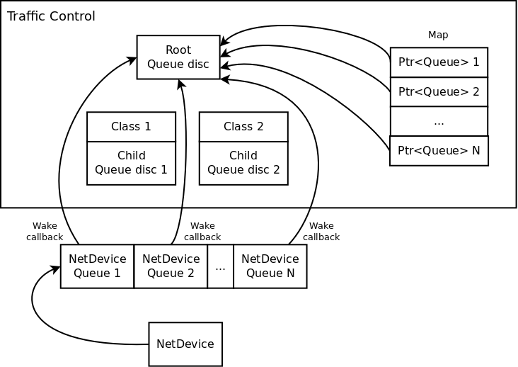
Setup of a queue disc (wake mode: WAKE_ROOT)
Setup of a multi-queue aware queue disc below shows instead how the TrafficControlLayer map looks like in case of a classful root queue disc whose wake mode is WAKE_CHILD.
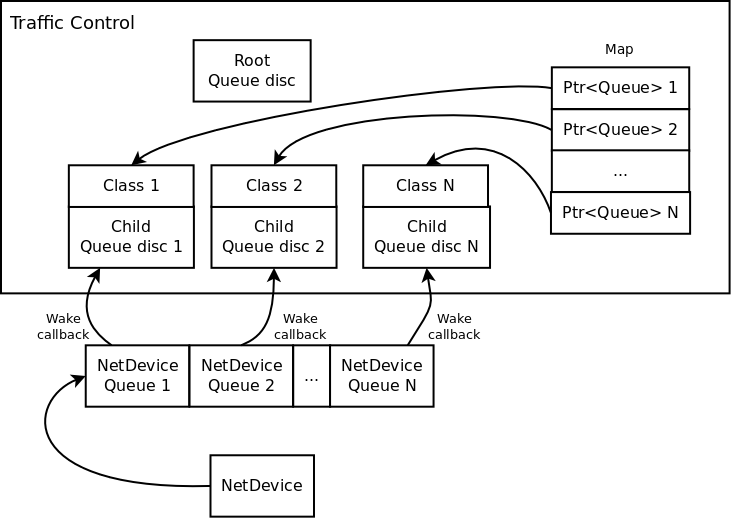
Setup of a multi-queue aware queue disc
A NetDeviceQueueInterface object is used by the traffic control layer to access the information stored in the NetDeviceQueue objects, retrieve the number of transmission queues of the device and get the transmission queue selected for the transmission of a given packet. A NetDeviceQueueInterface object must be therefore aggregated to all the devices having an interface supporting the traffic control layer (i.e., an IPv4 or IPv6 interface). In particular:
- a NetDeviceQueueInterface object is aggregated to all the devices by the NetDevice
helper classes, at
Installtime. See, for example, the implementation in the methodCsmaHelper::InstallPriv(). - when notified that a netdevice queue interface has been aggregated, traffic control aware devices can cache the pointer to the netdevice queue interface created by the traffic control layer into a member variable. Also, multi-queue devices can set the number of device transmission queues and set the select queue callback through the netdevice queue interface
- at initialization time, the traffic control (after calling device->Initialize () to ensure that the netdevice has set the number of device transmission queues, if it has to do so) completes the installation of the queue discs by setting the wake callbacks on the device transmission queues (through the netdevice queue interface). Also, the traffic control calls the Initialize method of the root queue discs. This initialization of queue discs triggers calls to the
CheckConfigandInitializeParamsmethods of the queue disc.
Requeue
In Linux, a packet dequeued from a queue disc can be requeued (i.e., stored somewhere and sent to the device at a later time) in some circumstances. Firstly, the function used to dequeue a packet (dequeue_skb) actually dequeues a packet only if the device is multi-queue or the (unique) device queue is not stopped. If a packet has been dequeued from the queue disc, it is passed to the sch_direct_xmit function for transmission to the device. This function checks whether the device queue the packet is destined to is stopped, in which case the packet is requeued. Otherwise, the packet is sent to the device. If the device returns NETDEV_TX_BUSY, the packet is requeued. However, it is advised that the function called to send a packet to the device (ndo_start_xmit) should always return NETDEV_TX_OK, which means that the packet is consumed by the device driver and thus needs not to be requeued. However, the ndo_start_xmit function of the device driver is allowed to return NETDEV_TX_BUSY (and hence the packet is requeued) when there is no room for the received packet in the device queue, despite the queue is not stopped. This case is considered as a corner case or an hard error, and should be avoided.
ns-3 implements the requeue mechanism in a similar manner, the only difference being that packets are not requeued when such corner cases occur. Basically, the method used to dequeue a packet (QueueDisc::DequeuePacket) actually dequeues a packet only if the device is multi-queue or the (unique) device queue is not stopped. If a packet has been dequeued from the queue disc, it is passed to the QueueDisc::Transmit method for transmission to the device. This method checks whether the device queue the packet is destined to is stopped, in which case the packet is requeued. Otherwise, the packet is sent to the device. We request netdevices to stop a device queue when it is not able to store another packet, so as to avoid the situation in which a packet is received that cannot be enqueued while the device queue is not stopped. Should such a corner case occur, the netdevice drops the packet but, unlike Linux, the value returned by NetDevice::Send is ignored and the packet is not requeued.
The way the requeue mechanism is implemented in ns-3 has the following implications:
- if the underlying device has a single queue, no packet will ever be requeued. Indeed, if the device queue is not stopped when QueueDisc::DequeuePacket is called, it will not be stopped also when QueueDisc::Transmit is called, hence the packet is not requeued (recall that a packet is not requeued after being sent to the device, as the value returned by NetDevice::Send is ignored).
- if the underlying device does not implement flow control, i.e., it does not stop its queue(s), no packet will ever be requeued (recall that a packet is only requeued by QueueDisc::Transmit when the device queue the packet is destined to is stopped)
It turns out that packets may only be requeued when the underlying device is multi-queue and supports flow control.
Fifo queue disc
Model Description
FifoQueueDisc implements the FIFO (First-In First-Out) policy. Packets are enqueued in the unique internal queue, which is implemented as a DropTail queue. The queue disc capacity can be specified in terms of either packets or bytes, depending on the value of the Mode attribute.
User is allowed to provide an internal queue before the queue disc is initialized. If no internal queue is provided, one DropTail queue having the same capacity of the queue disc is created by default. No packet filter can be added to a FifoQueueDisc.
Attributes
The FifoQueueDisc class holds the following attribute:
MaxSize:The maximum number of packets/bytes the queue disc can hold. The default value is 1000 packets.
Validation
The fifo model is tested using FifoQueueDiscTestSuite class defined
in src/traffic-control/test/fifo-queue-disc-test-suite.cc. The test aims to
check that the capacity of the queue disc is not exceeded and packets are dequeued
in the correct order.
pfifo_fast queue disc
Model Description
PfifoFastQueueDisc behaves like pfifo_fast, which is the default queue disc enabled on Linux systems (init systems such as systemd may override such default setting). Packets are enqueued in three priority bands (implemented as FIFO droptail queues) based on their priority (users can read Use of Send() vs. SendTo() for details on how to set packet priority). The four least significant bits of the priority are used to determine the selected band according to the following table:
| Priority & 0xf | Band |
|---|---|
| 0 | 1 |
| 1 | 2 |
| 2 | 2 |
| 3 | 2 |
| 4 | 1 |
| 5 | 2 |
| 6 | 0 |
| 7 | 0 |
| 8 | 1 |
| 9 | 1 |
| 10 | 1 |
| 11 | 1 |
| 12 | 1 |
| 13 | 1 |
| 14 | 1 |
| 15 | 1 |
The system behaves similar to three ns3::DropTail queues operating together, in which packets from higher priority bands are always dequeued before a packet from a lower priority band is dequeued.
The queue disc capacity, i.e., the maximum number of packets that can be enqueued in the queue disc, is set through the MaxSize attribute, which plays the same role as txqueuelen in Linux. If no internal queue is provided, three DropTail queues having each a capacity equal to MaxSize are created by default. User is allowed to provide queues, but they must be three, operate in packet mode and each have a capacity not less than MaxSize. No packet filter can be added to a PfifoFastQueueDisc.
Attributes
The PfifoFastQueueDisc class holds a single attribute:
MaxSize:The maximum number of packets accepted by the queue disc. The default value is 1000.
Examples
Various examples located in src/traffic-control/examples (e.g., codel-vs-pfifo-asymmetric.cc)
shows how to configure and install a PfifoFastQueueDisc on internet nodes.
Validation
The pfifo_fast model is tested using PfifoFastQueueDiscTestSuite class defined
in src/test/ns3tc/pfifo-fast-queue-disc-test-suite.cc. The suite includes 4 test cases:
- Test 1: The first test checks whether IPv4 packets are enqueued in the correct band based on the TOS byte
- Test 2: The second test checks whether IPv4 packets are enqueued in the correct band based on the TOS byte
- Test 3: The third test checks that the queue disc cannot enqueue more packets than its limit
- Test 4: The fourth test checks that packets that the filters have not been able to classify are enqueued into the default band of 1
Prio queue disc
Model Description
PrioQueueDisc implements a strict priority policy, where packets are dequeued from
a band only if higher priority bands are all empty. PrioQueueDisc is a classful
queue disc and can have an arbitrary number of bands, each of which is handled by a
queue disc of any kind. The capacity of PrioQueueDisc is not limited; packets can
only be dropped by child queue discs (which may have a limited capacity).
If no packet filter is installed or able to classify a packet, then the
packet is enqueued into a priority band based on its priority (modulo 16), which
is used as an index into an array called priomap. Users can read Use of Send() vs. SendTo()
for details on how to set the packet priority. If a packet is classified
by an installed packet filter and the returned value i is non-negative and less than the
number of priority bands, then the packet is enqueued into the i-th priority band.
Otherwise, the packet is enqueued into the priority band specified by the first element
of the priomap array.
If no queue disc class is added by the user before the queue disc is initialized, three child queue discs of type FifoQueueDisc are automatically added. It has to be noted that PrioQueueDisc needs at least two child queue discs.
Attributes
The PrioQueueDisc class holds the following attribute:
Priomap:The priority to band mapping. The default value is the same mapping as the (fixed) one used by PfifoFastQueueDisc.
Examples
An example of how to configure PrioQueueDisc with custom child queue discs and priomap
is provided by queue-discs-benchmark.cc located in examples/traffic-control:
TrafficControlHelper tch;
uint16_t handle = tch.SetRootQueueDisc ("ns3::PrioQueueDisc", "Priomap", StringValue ("0 1 0 1 0 1 0 1 0 1 0 1 0 1 0 1"));
TrafficControlHelper::ClassIdList cid = tch.AddQueueDiscClasses (handle, 2, "ns3::QueueDiscClass");
tch.AddChildQueueDisc (handle, cid[0], "ns3::FifoQueueDisc");
tch.AddChildQueueDisc (handle, cid[1], "ns3::RedQueueDisc");
The code above adds two classes (bands) to a PrioQueueDisc. The highest priority one is a FifoQueueDisc, the other one is a RedQueueDisc. The attribute Priomap is set to an array containing only 0 and 1 (since PrioQueueDisc only has two bands).
Validation
PrioQueueDisc is tested using PrioQueueDiscTestSuite class defined
in src/traffic-control/test/prio-queue-disc-test-suite.cc. The test aims to
check that: i) packets are enqueued in the correct band based on their priority and
the priomap or according to the value returned by the installed packet filter;
ii) packets are dequeued in the correct order.
The test suite can be run using the following commands:
$ ./waf configure --enable-examples --enable-tests
$ ./waf build
$ ./test.py -s prio-queue-disc
or
$ NS_LOG="PrioQueueDisc" ./waf --run "test-runner --suite=prio-queue-disc"
TBF queue disc
This chapter describes the TBF ([Ref1]) queue disc implementation in ns-3. The TBF model in ns-3 is ported based on Linux kernel code implemented by A. Kuznetsov and D. Torokhov.
TBF is a qdisc that allows controlling the bandwidth of the output according to a set rate with the possibility of managing burst conditions also. The TBF implementation consists of a bucket (buffer) having a limited capacity into which tokens (normally representing a unit of bytes or a single packet of predetermined size) are added at a fixed rate ‘r’ called the token rate. Whenever a packet arrives into the tx queue (fifo by default), the bucket is checked to see if there are appropriate number of tokens that is equivalent to the length of the packet in bytes. If yes, then the tokens are removed and the packet is passed for transmission. If no, then packets will have to wait until there are sufficient tokens in the bucket. This data conformance can be thus put into three possible scenarios [Ref3]:
- Data rate = Token rate : Packets pass without delay.
- Data rate < Token rate : The tokens might accumulate and the bucket might become full. Then, the next packets to enter TBF will be transmitted right away without having any limit applied to them, until the bucket is empty. This is called a burst condition and in TBF the burst parameter defines the size of the bucket. In order to overcome this problem and provide better control over the bursts, TBF implements a second bucket which is smaller and generally the same size as the MTU. This second bucket cannot store large amount of tokens, but its replenishing rate will be a lot faster than the one of the big bucket. This second rate is called ‘peakRate’ and it will determine the maximum rate of a burst.
- Data rate > Token rate : This causes the TBF algorithm to throttle itself for a while as soon as the bucket gets empty. This is called an ‘overlimit situation’ [Ref2]. In this situation, some of the packets will be blocked until enough tokens are available at which time a schedule for the waking of the queue will be done. If packets keep coming in, at a larger rate, then the packets will start to get dropped when the total number of bytes exceeds the QueueLimit.
Model Description
The TBF queue disc does not require packet filters, does not admit internal queues and uses a single child queue disc. If the user does not provide a child queue disc, a Fifo queue disc operating in the same mode (packet or byte) as the TBF queue disc and having a size equal to the TBF QueueLimit attribute is created. Otherwise, the capacity of the TBF queue disc is determined by the capacity of the child queue disc.
There are two token buckets: first bucket and second bucket. The size of the first bucket called ‘Burst’ should always be greater than the size of the second bucket called the Mtu (which is usually the size of a single packet). But the ‘PeakRate’ which is the second bucket’s token rate should be always greater than the ‘Rate’ which is the first bucket’s token rate.
If the PeakRate is zero, then the second bucket does not exist. In order to activate the second bucket, both the Mtu and PeakRate values have to be greater than zero. If the Mtu value is zero at initialization time, then if a NetDevice exits, the Mtu’s value will be equal to the Mtu of the NetDevice. But if no NetDevice exists, then the QueueDisc will complain thus prompting the user to set the Mtu value.
The source code for the TBF model is located in the directory src/traffic-control/model
and consists of 2 files tbf-queue-disc.h and tbf-queue-disc.cc defining a TbfQueueDisc
class.
- class
TbfQueueDisc: This class implements the main TBF algorithm:TbfQueueDisc::DoEnqueue (): This routine enqueue’s the incoming packet if the queue is not full and drops the packet otherwise.TbfQueueDisc::DoPeek (): This routine peeks for the top item in the queue and if the queue is not empty, it returns the topmost item.TbfQueueDisc::DoDequeue (): This routine performs the dequeuing of packets according to the following logic:- It calls
TbfQueueDisc::Peek ()and calculates the size of the packet to be dequeued in bytes. - Then it calculates the time difference ‘delta’, which is the time elapsed since the last update of tokens in the buckets.
- If the second bucket exists, the number of tokens are updated according to the ‘PeakRate’ and ‘delta’.
- From this second bucket a number of tokens equal to the size of the packet to be dequeued is subtracted.
- Now the number of tokens in the first bucket are updated according to ‘Rate’ and ‘delta’.
- From this first bucket a number of tokens equal to the size of the packet to be dequeued is subtracted.
- If after this, both the first and second buckets have tokens greater than zero, then the packet is dequeued.
- Else, an event to
QueueDisc::Run ()is scheduled after a time period when enough tokens will be present for the dequeue operation.
- It calls
References
| [Ref1] |
|
| [Ref2] |
|
| [Ref3] | Practical IP Network QoS: TBF queuing discipline; Available online at http://web.opalsoft.net/qos/default.php?p=ds-24. |
Attributes
The key attributes that the TbfQueueDisc class holds include the following:
MaxSize:The maximum number of packets/bytes the queue disc can hold. The default value is 1000 packets.Burst:Size of the first bucket, in bytes. The default value is 125000 bytes.Mtu:Size of second bucket defaults to the MTU of the attached NetDevice, if any, or 0 otherwise.Rate:Rate at which tokens enter the first bucket. The default value is 125KB/s.PeakRate:Rate at which tokens enter the second bucket. The default value is 0KB/s, which means that there is no second bucket.
TraceSources
The TbfQueueDisc class provides the following trace sources:
TokensInFirstBucket:Number of First Bucket Tokens in bytesTokensInSecondBucket:Number of Second Bucket Tokens in bytes
Examples
The example for TBF is tbf-example.cc located in examples/traffic-control/. The command to run the file (the invocation below shows the available command-line options) is:
.. sourcecode:: bash
$ ./waf –run “tbf-example –PrintHelp” $ ./waf –run “tbf-example –burst=125000 –rate=1Mbps –peakRate=1.5Mbps”
The expected output from the previous commands are traced value changes in the number of tokens in the first and second buckets.
Validation
The TBF model is tested using TbfQueueDiscTestSuite class defined in src/traffic-control/test/tbf-queue-disc-test-suite.cc. The suite includes 4 test cases:
- Test 1: Simple Enqueue/Dequeue with verification of attribute setting and subtraction of tokens from the buckets.
- Test 2: When DataRate == FirstBucketTokenRate; packets should pass smoothly.
- Test 3: When DataRate >>> FirstBucketTokenRate; some packets should get blocked and waking of queue should get scheduled.
- Test 4: When DataRate < FirstBucketTokenRate; burst condition, peakRate is set so that bursts are controlled.
The test suite can be run using the following commands:
.. sourcecode:: bash
$ ./waf configure –enable-examples –enable-tests $ ./waf build $ ./test.py -s tbf-queue-disc
or
.. sourcecode:: bash
$ NS_LOG=”TbfQueueDisc” ./waf –run “test-runner –suite=tbf-queue-disc”
RED queue disc
Model Description
Random Early Detection (RED) is a queue discipline that aims to provide early signals to transport protocol congestion control (e.g. TCP) that congestion is imminent, so that they back off their rate gracefully rather than with a bunch of tail-drop losses (possibly incurring TCP timeout). The model in ns-3 is a port of Sally Floyd’s ns-2 RED model.
Note that, starting from ns-3.25, RED is no longer a queue variant and cannot be installed as a NetDevice queue. Instead, RED is a queue disc and must be installed in the context of the traffic control (see the examples mentioned below).
The RED queue disc does not require packet filters, does not admit child queue discs and uses a single internal queue. If not provided by the user, a DropTail queue operating in the same mode (packet or byte) as the queue disc and having a size equal to the RED MaxSize attribute is created. Otherwise, the capacity of the queue disc is determined by the capacity of the internal queue provided by the user.
Adaptive Random Early Detection (ARED)
ARED is a variant of RED with two main features: (i) automatically sets Queue weight, MinTh and MaxTh and (ii) adapts maximum drop probability. The model in ns-3 contains implementation of both the features, and is a port of Sally Floyd’s ns-2 ARED model. Note that the user is allowed to choose and explicitly configure the simulation by selecting feature (i) or feature (ii), or both.
Feng’s Adaptive RED
Feng’s Adaptive RED is a variant of RED that adapts the maximum drop probability. The model in ns-3 contains implementation of this feature, and is a port of ns-2 Feng’s Adaptive RED model.
Nonlinear Random Early Detection (NLRED)
NLRED is a variant of RED in which the linear packet dropping function of RED is replaced by a nonlinear quadratic function. This approach makes packet dropping gentler for light traffic load and aggressive for heavy traffic load.
Explicit Congestion Notification (ECN)
This RED model supports an ECN mode of operation to notify endpoints of congestion that may be developing in a bottleneck queue, without resorting to packet drops. Such a mode is enabled by setting the UseEcn attribute to true (it is false by default) and only affects incoming packets with the ECT bit set in their header. When the average queue length is between the minimum and maximum thresholds, an incoming packet is marked instead of being dropped. When the average queue length is above the maximum threshold, an incoming packet is marked (instead of being dropped) only if the UseHardDrop attribute is set to false (it is true by default).
The implementation of support for ECN marking is done in such a way as
to not impose an internet module dependency on the traffic control module.
The RED model does not directly set ECN bits on the header, but delegates
that job to the QueueDiscItem class. As a result, it is possible to
use RED queues for other non-IP QueueDiscItems that may or may not support
the Mark () method.
References
The RED queue disc aims to be close to the results cited in: S.Floyd, K.Fall http://icir.org/floyd/papers/redsims.ps
ARED queue implementation is based on the algorithm provided in: S. Floyd et al, http://www.icir.org/floyd/papers/adaptiveRed.pdf
Feng’s Adaptive RED queue implementation is based on the algorithm provided in: W. C. Feng et al, http://ieeexplore.ieee.org/stamp/stamp.jsp?arnumber=752150
NLRED queue implementation is based on the algorithm provided in: Kaiyu Zhou et al, http://www.sciencedirect.com/science/article/pii/S1389128606000879
The addition of explicit congestion notification (ECN) to IP: K. K. Ramakrishnan et al, https://tools.ietf.org/html/rfc3168
Attributes
The RED queue contains a number of attributes that control the RED policies:
- MaxSize
- MeanPktSize
- IdlePktSize
- Wait (time)
- Gentle mode
- MinTh, MaxTh
- Queue weight
- LInterm
- LinkBandwidth
- LinkDelay
- UseEcn
- UseHardDrop
In addition to RED attributes, ARED queue requires following attributes:
- ARED (Boolean attribute. Default: false)
- AdaptMaxP (Boolean attribute to adapt m_curMaxP. Default: false)
- Target Delay (time)
- Interval (time)
- LastSet (time)
- Top (upper limit of m_curMaxP)
- Bottom (lower limit of m_curMaxP)
- Alpha (increment parameter for m_curMaxP)
- Beta (decrement parameter for m_curMaxP)
- RTT
In addition to RED attributes, Feng’s Adaptive RED queue requires following attributes:
- FengAdaptive (Boolean attribute, Default: false)
- Status (status of current queue length, Default: Above)
- FengAlpha (increment parameter for m_curMaxP, Default: 3)
- FengBeta (decrement parameter for m_curMaxP, Default: 2)
The following attribute should be turned on to simulate NLRED queue disc:
- NLRED (Boolean attribute. Default: false)
Consult the ns-3 documentation for explanation of these attributes.
Simulating ARED
To switch on ARED algorithm, the attribute ARED must be set to true,
as done in src/traffic-control/examples/adaptive-red-tests.cc:
Config::SetDefault ("ns3::RedQueueDisc::ARED", BooleanValue (true));
Setting ARED to true implicitly configures both: (i) automatic setting of Queue weight, MinTh and MaxTh and (ii) adapting m_curMaxP.
NOTE: To explicitly configure (i) or (ii), set ARED attribute to false and follow the procedure described next:
To configure (i); Queue weight, MinTh and MaxTh, all must be set to 0,
as done in src/traffic-control/examples/adaptive-red-tests.cc:
Config::SetDefault ("ns3::RedQueueDisc::QW", DoubleValue (0.0));
Config::SetDefault ("ns3::RedQueueDisc::MinTh", DoubleValue (0));
Config::SetDefault ("ns3::RedQueueDisc::MaxTh", DoubleValue (0));
To configure (ii); AdaptMaxP must be set to true, as done in
src/traffic-control/examples/adaptive-red-tests.cc:
Config::SetDefault ("ns3::RedQueueDisc::AdaptMaxP", BooleanValue (true));
Simulating Feng’s Adaptive RED
To switch on Feng’s Adaptive RED algorithm, the attribute FengAdaptive must be
set to true, as done in examples/traffic-control/red-vs-fengadaptive.cc:
Config::SetDefault ("ns3::RedQueueDisc::FengAdaptive", BooleanValue (true));
Simulating NLRED
To switch on NLRED algorithm, the attribute NLRED must be set to true, as shown below:
Config::SetDefault ("ns3::RedQueueDisc::NLRED", BooleanValue (true));
Examples
The RED queue example is found at src/traffic-control/examples/red-tests.cc.
ARED queue examples can be found at:
src/traffic-control/examples/adaptive-red-tests.cc and
src/traffic-control/examples/red-vs-ared.cc
Feng’s Adaptive RED example can be found at:
examples/traffic-control/red-vs-fengadaptive.cc
NLRED queue example can be found at:
examples/traffic-control/red-vs-nlred.cc
Validation
The RED model has been validated and the report is currently stored at: https://github.com/downloads/talau/ns-3-tcp-red/report-red-ns3.pdf
CoDel queue disc
This chapter describes the CoDel ([Nic12], [Nic14]) queue disc implementation in ns-3.
Developed by Kathleen Nichols and Van Jacobson as a solution to the bufferbloat [Buf14] problem, CoDel (Controlled Delay Management) is a queuing discipline that uses a packet’s sojourn time (time in queue) to make decisions on packet drops.
Note that, starting from ns-3.25, CoDel is no longer a queue variant and cannot be installed as a NetDevice queue. Instead, CoDel is a queue disc and must be installed in the context of the traffic control (see the examples mentioned below).
Model Description
The source code for the CoDel model is located in the directory src/traffic-control/model
and consists of 2 files codel-queue-disc.h and codel-queue-disc.cc defining a CoDelQueueDisc
class and a helper CoDelTimestampTag class. The code was ported to ns-3 by
Andrew McGregor based on Linux kernel code implemented by Dave Täht and Eric Dumazet.
- class
CoDelQueueDisc: This class implements the main CoDel algorithm:CoDelQueueDisc::DoEnqueue (): This routine tags a packet with the current time before pushing it into the queue. The timestamp tag is used byCoDelQueue::DoDequeue()to compute the packet’s sojourn time. If the queue is full upon the packet arrival, this routine will drop the packet and record the number of drops due to queue overflow, which is stored in m_dropOverLimit.CoDelQueueDisc::ShouldDrop (): This routine isCoDelQueueDisc::DoDequeue()’s helper routine that determines whether a packet should be dropped or not based on its sojourn time. If the sojourn time goes above m_target and remains above continuously for at least m_interval, the routine returnstrueindicating that it is OK to drop the packet. Otherwise, it returnsfalse.CoDelQueueDisc::DoDequeue (): This routine performs the actual packet drop based onCoDelQueueDisc::ShouldDrop ()’s return value and schedules the next drop/mark.
- class
CoDelTimestampTag: This class implements the timestamp tagging for a packet. This tag is used to compute the packet’s sojourn time (the difference between the time the packet is dequeued and the time it is pushed into the queue).
There are 2 branches to CoDelQueueDisc::DoDequeue ():
If the queue is currently in the dropping state, which means the sojourn time has remained above m_target for more than m_interval, the routine determines if it’s OK to leave the dropping state or it’s time for the next drop/mark. When
CoDelQueueDisc::ShouldDrop ()returnsfalse, the queue can move out of the dropping state (set m_dropping tofalse). Otherwise, the queue continuously drops/marks packets and updates the time for next drop (m_dropNext) until one of the following conditions is met:- The queue is empty, upon which the queue leaves the dropping state and exits
CoDelQueueDisc::ShouldDrop ()routine; CoDelQueueDisc::ShouldDrop ()returnsfalse(meaning the sojourn time goes below m_target) upon which the queue leaves the dropping state;- It is not yet time for next drop/mark (m_dropNext is less than current time) upon which the queue waits for the next packet dequeue to check the condition again.
- The queue is empty, upon which the queue leaves the dropping state and exits
If the queue is not in the dropping state, the routine enters the dropping state and drop/mark the first packet if
CoDelQueueDisc::ShouldDrop ()returnstrue(meaning the sojourn time has gone above m_target for at least m_interval for the first time or it has gone above again after the queue leaves the dropping state).
The CoDel queue disc does not require packet filters, does not admit child queue discs and uses a single internal queue. If not provided by the user, a DropTail queue operating in the same mode (packet or byte) as the queue disc and having a size equal to the CoDel MaxSize attribute is created. Otherwise, the capacity of the queue disc is determined by the capacity of the internal queue provided by the user.
References
| [Nic12] |
|
| [Nic14] |
|
| [Buf14] | Bufferbloat.net. Available online at http://www.bufferbloat.net/. |
Attributes
The key attributes that the CoDelQueue class holds include the following:
MaxSize:The maximum number of packets/bytes the queue can hold. The default value is 1500 * DEFAULT_CODEL_LIMIT, which is 1500 * 1000 bytes.MinBytes:The CoDel algorithm minbytes parameter. The default value is 1500 bytes.Interval:The sliding-minimum window. The default value is 100 ms.Target:The CoDel algorithm target queue delay. The default value is 5 ms.UseEcn:True to use ECN (packets are marked instead of being dropped). The default value is false.CeThreshold:The CoDel CE threshold for marking packets. Disabled by default.
Examples
The first example is codel-vs-pfifo-basic-test.cc located in src/traffic-control/examples. To run the file (the first invocation below shows the available
command-line options):
$ ./waf --run "codel-vs-pfifo-basic-test --PrintHelp"
$ ./waf --run "codel-vs-pfifo-basic-test --queueType=CoDel --pcapFileName=codel.pcap --cwndTrFileName=cwndCodel.tr"
The expected output from the previous commands are two files: codel.pcap file and cwndCoDel.tr (ASCII trace) file The .pcap file can be analyzed using wireshark or tcptrace:
$ tcptrace -l -r -n -W codel.pcap
The second example is codel-vs-pfifo-asymmetric.cc located in src/traffic-control/examples. This example is intended to model a typical cable modem
deployment scenario. To run the file:
$ ./waf --run "codel-vs-pfifo-asymmetric --PrintHelp"
$ ./waf --run codel-vs-pfifo-asymmetric
The expected output from the previous commands is six pcap files:
- codel-vs-pfifo-asymmetric-CoDel-server-lan.pcap
- codel-vs-pfifo-asymmetric-CoDel-router-wan.pcap
- codel-vs-pfifo-asymmetric-CoDel-router-lan.pcap
- codel-vs-pfifo-asymmetric-CoDel-cmts-wan.pcap
- codel-vs-pfifo-asymmetric-CoDel-cmts-lan.pcap
- codel-vs-pfifo-asymmetric-CoDel-host-lan.pcap
One attribute file:
- codel-vs-pfifo-asymmetric-CoDel.attr
Five ASCII trace files:
- codel-vs-pfifo-asymmetric-CoDel-drop.tr
- codel-vs-pfifo-asymmetric-CoDel-drop-state.tr
- codel-vs-pfifo-asymmetric-CoDel-sojourn.tr
- codel-vs-pfifo-asymmetric-CoDel-length.tr
- codel-vs-pfifo-asymmetric-CoDel-cwnd.tr
Validation
The CoDel model is tested using CoDelQueueDiscTestSuite class defined in src/traffic-control/test/codel-queue-test-suite.cc. The suite includes 5 test cases:
- Test 1: The first test checks the enqueue/dequeue with no drops and makes sure that CoDel attributes can be set correctly.
- Test 2: The second test checks the enqueue with drops due to queue overflow.
- Test 3: The third test checks the NewtonStep() arithmetic against explicit port of Linux implementation
- Test 4: The fourth test checks the ControlLaw() against explicit port of Linux implementation
- Test 5: The fifth test checks the enqueue/dequeue with drops according to CoDel algorithm
- Test 6: The sixth test checks the enqueue/dequeue with marks according to CoDel algorithm
The test suite can be run using the following commands:
$ ./waf configure --enable-examples --enable-tests
$ ./waf build
$ ./test.py -s codel-queue-disc
or
$ NS_LOG="CoDelQueueDisc" ./waf --run "test-runner --suite=codel-queue-disc"
FqCoDel queue disc
This chapter describes the FqCoDel ([Hoe16]) queue disc implementation in ns-3.
The FlowQueue-CoDel (FQ-CoDel) algorithm is a combined packet scheduler and Active Queue Management (AQM) algorithm developed as part of the bufferbloat-fighting community effort ([Buf16]). FqCoDel classifies incoming packets into different queues (by default, 1024 queues are created), which are served according to a modified Deficit Round Robin (DRR) queue scheduler. Each queue is managed by the CoDel AQM algorithm. FqCoDel distinguishes between “new” queues (which don’t build up a standing queue) and “old” queues, that have queued enough data to be around for more than one iteration of the round-robin scheduler.
FqCoDel is installed by default on single-queue NetDevices (such as PointToPoint, Csma and Simple). Also, on multi-queue devices (such as Wifi), the default root qdisc is Mq with as many FqCoDel child queue discs as the number of device queues.
Model Description
The source code for the FqCoDel queue disc is located in the directory
src/traffic-control/model and consists of 2 files fq-codel-queue-disc.h
and fq-codel-queue-disc.cc defining a FqCoDelQueueDisc class and a helper
FqCoDelFlow class. The code was ported to ns-3 based on Linux kernel code
implemented by Eric Dumazet.
Set associative hashing is also based on the Linux kernel CAKE queue management code.
Set associative hashing is used to reduce the number of hash collisions in
comparison to choosing queues normally with a simple hash. For a given number of
queues, set associative hashing has fewer collisions than a traditional
hash, as long as the number of flows is lesser than the number of queues.
Essentially, it makes the queue management system more efficient. Set associative
hashing is a vital component of CAKE, which is another popular flow management
algorithm that is implemented in Linux and is being tested for FqCoDel.
Furthermore, this module can be directly used with CAKE when its other
components are implemented in ns-3. The only changes needed to incorporate this
new hashing scheme are in the SetAssociativeHash and DoEnqueue methods,
as described below.
- class
FqCoDelQueueDisc: This class implements the main FqCoDel algorithm:FqCoDelQueueDisc::DoEnqueue (): If no packet filter has been configured, this routine calls the QueueDiscItem::Hash() method to classify the given packet into an appropriate queue. Otherwise, the configured filters are used to classify the packet. If the filters are unable to classify the packet, the packet is dropped. Otherwise, an option is provided if set associative hashing is to be used.The packet is now handed over to the CoDel algorithm for timestamping. Then, if the queue is not currently active (i.e., if it is not in either the list of new or the list of old queues), it is added to the end of the list of new queues, and its deficit is initiated to the configured quantum. Otherwise, the queue is left in its current queue list. Finally, the total number of enqueued packets is compared with the configured limit, and if it is above this value (which can happen since a packet was just enqueued), packets are dropped from the head of the queue with the largest current byte count until the number of dropped packets reaches the configured drop batch size or the backlog of the queue has been halved. Note that this in most cases means that the packet that was just enqueued is not among the packets that get dropped, which may even be from a different queue.FqCoDelQueueDisc::SetAssociativeHash(): An outer hash is identified for the given packet. This corresponds to the set into which the packet is to be enqueued. A set consists of a group of queues. The set determined by outer hash is enumerated; if a queue corresponding to this packet’s flow is found (we use per-queue tags to achieve this), or in case of an inactive queue, or if a new queue can be created for this set without exceeding the maximum limit, the index of this queue is returned. Otherwise, all queues of this full set are active and correspond to flows different from the current packet’s flow. In such cases, the index of first queue of this set is returned. We don’t consider creating new queues for the packet in these cases, since this approach may waste resources in the long run. The situation highlighted is a guaranteed collision and cannot be avoided without increasing the overall number of queues.FqCoDelQueueDisc::DoDequeue (): The first task performed by this routine is selecting a queue from which to dequeue a packet. To this end, the scheduler first looks at the list of new queues; for the queue at the head of that list, if that queue has a negative deficit (i.e., it has already dequeued at least a quantum of bytes), it is given an additional amount of deficit, the queue is put onto the end of the list of old queues, and the routine selects the next queue and starts again. Otherwise, that queue is selected for dequeue. If the list of new queues is empty, the scheduler proceeds down the list of old queues in the same fashion (checking the deficit, and either selecting the queue for dequeuing, or increasing deficit and putting the queue back at the end of the list). After having selected a queue from which to dequeue a packet, the CoDel algorithm is invoked on that queue. As a result of this, one or more packets may be discarded from the head of the selected queue, before the packet that should be dequeued is returned (or nothing is returned if the queue is or becomes empty while being handled by the CoDel algorithm). Finally, if the CoDel algorithm does not return a packet, then the queue must be empty, and the scheduler does one of two things: if the queue selected for dequeue came from the list of new queues, it is moved to the end of the list of old queues. If instead it came from the list of old queues, that queue is removed from the list, to be added back (as a new queue) the next time a packet for that queue arrives. Then (since no packet was available for dequeue), the whole dequeue process is restarted from the beginning. If, instead, the scheduler did get a packet back from the CoDel algorithm, it subtracts the size of the packet from the byte deficit for the selected queue and returns the packet as the result of the dequeue operation.FqCoDelQueueDisc::FqCoDelDrop (): This routine is invoked byFqCoDelQueueDisc::DoEnqueue()to drop packets from the head of the queue with the largest current byte count. This routine keeps dropping packets until the number of dropped packets reaches the configured drop batch size or the backlog of the queue has been halved.
- class
FqCoDelFlow: This class implements a flow queue, by keeping its current status (whether it is in the list of new queues, in the list of old queues or inactive) and its current deficit.
In Linux, by default, packet classification is done by hashing (using a Jenkins hash function) the 5-tuple of IP protocol, source and destination IP addresses and port numbers (if they exist). This value modulo the number of queues is salted by a random value selected at initialization time, to prevent possible DoS attacks if the hash is predictable ahead of time. Alternatively, any other packet filter can be configured. In ns-3, packet classification is performed in the same way as in Linux. Neither internal queues nor classes can be configured for an FqCoDel queue disc.
Possible next steps
- what to do if ECT(1) and either/both ECT(0) and NotECT are in the same flow queue (hash collisions or tunnels)– our L4S traffic flows will avoid this situation by supporting AccECN and ECN++ (and if it happens in practice, the CoDel logic will just apply two separate thresholds)
- adding a ramp marking response instead of step threshold
- adding a floor value (to suppress marks if the queue length is below a certain number of bytes or packets)
- adding a heuristic such as in PIE to avoid marking a packet if it arrived to an empty flow queue (check on ingress, remember at egress time)
References
| [Hoe16] |
|
| [Buf16] | Bufferbloat.net. Available online at http://www.bufferbloat.net/. |
Attributes
The key attributes that the FqCoDelQueue class holds include the following:
UseEcn:True to use ECN (packets are marked instead of being dropped)Interval:The interval parameter to be used on the CoDel queues. The default value is 100 ms.Target:The target parameter to be used on the CoDel queues. The default value is 5 ms.MaxSize:The limit on the maximum number of packets stored by FqCoDel.Flows:The number of flow queues managed by FqCoDel.DropBatchSize:The maximum number of packets dropped from the fat flow.Perturbation:The salt used as an additional input to the hash function used to classify packets.CeThresholdThe FqCoDel CE threshold for marking packetsUseL4sTrue to use L4S (only ECT1 packets are marked at CE threshold)EnableSetAssociativeHash:The parameter used to enable set associative hash.
Perturbation is an optional configuration attribute and can be used to generate different hash outcomes for different inputs. For instance, the tuples used as input to the hash may cause hash collisions (mapping to the same bucket) for a given set of inputs, but by changing the perturbation value, the same hash inputs now map to distinct buckets.
Note that the quantum, i.e., the number of bytes each queue gets to dequeue on
each round of the scheduling algorithm, is set by default to the MTU size of the
device (at initialisation time). The FqCoDelQueueDisc::SetQuantum () method
can be used (at any time) to configure a different value.
Examples
A typical usage pattern is to create a traffic control helper and to configure type and attributes of queue disc and filters from the helper. For example, FqCodel can be configured as follows:
TrafficControlHelper tch;
tch.SetRootQueueDisc ("ns3::FqCoDelQueueDisc", "DropBatchSize", UintegerValue (1)
"Perturbation", UintegerValue (256));
QueueDiscContainer qdiscs = tch.Install (devices);
The example for FqCoDel’s L4S mode is FqCoDel-L4S-example.cc located in src/traffic-control/examples. To run the file (the first invocation below shows the available
command-line options):
$ ./waf --run "FqCoDel-L4S-example --PrintHelp"
$ ./waf --run "FqCoDel-L4S-example --scenarioNum=5"
The expected output from the previous command are .dat files.
Validation
The FqCoDel model is tested using FqCoDelQueueDiscTestSuite class defined in src/test/ns3tc/codel-queue-test-suite.cc. The suite includes 5 test cases:
- Test 1: The first test checks that packets that cannot be classified by any available filter are dropped.
- Test 2: The second test checks that IPv4 packets having distinct destination addresses are enqueued into different flow queues. Also, it checks that packets are dropped from the fat flow in case the queue disc capacity is exceeded.
- Test 3: The third test checks the dequeue operation and the deficit round robin-based scheduler.
- Test 4: The fourth test checks that TCP packets with distinct port numbers are enqueued into different flow queues.
- Test 5: The fifth test checks that UDP packets with distinct port numbers are enqueued into different flow queues.
- Test 6: The sixth test checks that the packets are marked correctly.
- Test 7: The seventh test checks the working of set associative hashing and its linear probing capabilities by using TCP packets with different hashes enqueued into different sets and queues.
- Test 8: The eighth test checks the L4S mode of FqCoDel where ECT1 packets are marked at CE threshold (target delay does not matter) while ECT0 packets continue to be marked at target delay (CE threshold does not matter).
The test suite can be run using the following commands:
$ ./waf configure --enable-examples --enable-tests
$ ./waf build
$ ./test.py -s fq-codel-queue-disc
or:
$ NS_LOG="FqCoDelQueueDisc" ./waf --run "test-runner --suite=fq-codel-queue-disc"
Set associative hashing is tested by generating a probability collision graph. This graph is then overlapped with the theoretical graph provided in the original CAKE paper (refer to Figure 1 from CAKE). The generated graph is linked below:
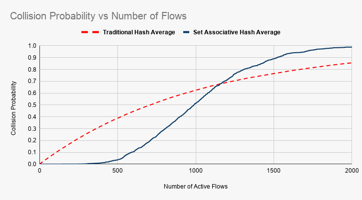
The overlapped graph is also linked below:
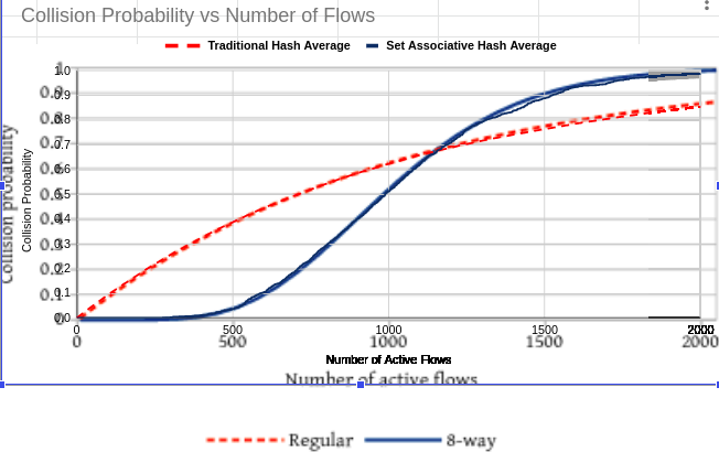
The steps to replicate this graph are available on this link.
Cobalt queue disc
This chapter describes the COBALT (CoDel BLUE Alternate) ([Cake16]) queue disc implementation in ns-3.
COBALT queue disc is an integral component of CAKE smart queue management system. It is a combination of the CoDel ([Kath17]) and BLUE ([BLUE02]) Active Queue Management algorithms.
Model Description
The source code for the COBALT model is located in the directory
src/traffic-control/model and consists of 2 files: cobalt-queue-disc.h and
cobalt-queue-disc.cc defining a CobaltQueueDisc class and a helper
CobaltTimestampTag class. The code was ported to ns-3 by Vignesh Kanan,
Harsh Lara, Shefali Gupta, Jendaipou Palmei and Mohit P. Tahiliani based on
the Linux kernel code.
Stefano Avallone and Pasquale Imputato helped in verifying the correctness of COBALT model in ns-3 by comparing the results obtained from it to those obtained from the Linux model of COBALT. A detailed comparison of ns-3 model of COBALT with Linux model of COBALT is provided in ([Cobalt19]).
- class
CobaltQueueDisc: This class implements the main Cobalt algorithm: CobaltQueueDisc::DoEnqueue (): This routine tags a packet with the current time before pushing it into the queue. The timestamp tag is used byCobaltQueue::DoDequeue()to compute the packet’s sojourn time. If the queue is full upon the packet arrival, this routine will drop the packet and record the number of drops due to queue overflow, which is stored in m_stats.qLimDrop.CobaltQueueDisc::ShouldDrop (): This routine isCobaltQueueDisc::DoDequeue()’s helper routine that determines whether a packet should be dropped or not based on its sojourn time. If L4S mode is enabled then if the packet is ECT1 is checked and if delay is greater than CE threshold then the packet is marked and returnsfalse. If the sojourn time goes above m_target and remains above continuously for at least m_interval, the routine returnstrueindicating that it is OK to drop the packet.Otherwise, it returns ``false. If L4S mode is turned off and CE threshold marking is enabled, then if the delay is greater than CE threshold, packet is marked. This routine decides if a packet should be dropped based on the dropping state of CoDel and drop probability of BLUE. The idea is to have both algorithms running in parallel and their effectiveness is decided by their respective parameters (Pdrop of BLUE and dropping state of CoDel). If either of them decide to drop the packet, the packet is dropped.CobaltQueueDisc::DoDequeue (): This routine performs the actual packetdrop based on ``CobaltQueueDisc::ShouldDrop ()’s return value and schedules the next drop. Cobalt will decrease BLUE’s drop probability if the queue is empty. This will ensure that the queue does not underflow. Otherwise Cobalt will take the next packet from the queue and calculate its drop state by running CoDel and BLUE in parallel till there are none left to drop.
References
| [Cake16] | Linux implementation of Cobalt as a part of the cake framework. Available online at https://github.com/dtaht/sch_cake/blob/master/cobalt.c. |
| [Kath17] | Controlled Delay Active Queue Management (draft-ietf-aqm-fq-codel-07) Available online at https://tools.ietf.org/html/draft-ietf-aqm-codel-07. |
| [BLUE02] | Feng, W. C., Shin, K. G., Kandlur, D. D., & Saha, D. (2002). The BLUE Active Queue Management Algorithms. IEEE/ACM Transactions on Networking (ToN), 10(4), 513-528. |
| [Cobalt19] | Jendaipou Palmei, Shefali Gupta, Pasquale Imputato, Jonathan Morton, Mohit P. Tahiliani, Stefano Avallone and Dave Taht (2019). Design and Evaluation of COBALT Queue Discipline. IEEE International Symposium on Local and Metropolitan Area Networks (LANMAN), July 2019. |
Attributes
The key attributes that the CobaltQueue Disc class holds include the following:
MaxSize:The maximum number of packets/bytes accepted by this queue disc.Interval:The sliding-minimum window. The default value is 100 ms.Target:The Cobalt algorithm target queue delay. The default value is 5 ms.Pdrop:Value of drop probability.Increment:Increment value of drop probability. Default value is 1./256 .Decrement:Decrement value of drop probability. Default value is 1./4096 .CeThreshold:The CoDel CE threshold for marking packets.UseL4s:True to use L4S (only ECT1 packets are marked at CE threshold).Count:Cobalt count.DropState:Dropping state of Cobalt. Default value is false.Sojourn:Per packet time spent in the queue.DropNext:Time until next packet drop.
Examples
An example program named cobalt-vs-codel.cc is located in
src/traffic-control/examples. Use the following command to run the program.
$ ./waf --run cobalt-vs-codel
Validation
The COBALT model is tested using CobaltQueueDiscTestSuite class
defined in src/traffic-control/test/cobalt-queue-test-suite.cc.
The suite includes 2 test cases:
- Test 1: Simple enqueue/dequeue with no drops.
- Test 2: Change of BLUE’s drop probability upon queue full (Activation of Blue).
- Test 3: This test verfies ECN marking.
- Test 4: CE threshold marking test.
The test suite can be run using the following commands:
$ ./waf configure --enable-examples --enable-tests
$ ./waf build
$ ./test.py -s cobalt-queue-disc
or
$ NS_LOG="CobaltQueueDisc" ./waf --run "test-runner --suite=cobalt-queue-disc"
FqCobalt queue disc
This chapter describes the FqCobalt ([Pal19]) queue disc implementation in ns-3.
The FlowQueue-Cobalt (FQ-Cobalt) algorithm is similar to FlowQueue-CoDel (FQ-CoDel) algorithm available in :FqCoDel queue disc.
The documentation for Cobalt is available in
ns-3-dev/src/traffic-control/doc/cobalt.rst.
FqCobalt is one of the key components of the CAKE smart queue management framework ([Hoe18]). The COBALT AQM is preferred to the CoDel AQM for CAKE because it adds a heuristic called BLUE to cover cases in which the CoDel control law is too sluggish to respond to queue growth.
Model Description
The source code for the FqCobalt queue disc is located in the directory
src/traffic-control/model and consists of 2 files fq-cobalt-queue-disc.h
and fq-cobalt-queue-disc.cc defining a FqCobaltQueueDisc class and a helper
FqCobaltFlow class. The code was ported to ns-3 based on Linux kernel code
implemented by Jonathan Morton
(https://github.com/torvalds/linux/blob/master/net/sched/sch_cake.c).
The Model Description is similar to the FqCoDel documentation mentioned above.
References
| [Pal19] |
|
| [Hoe18] |
|
Attributes
Most of the key attributes are similar to the FqCoDel implementation mentioned above. One difference is the absence of the MinBytes parameter.
Some additional parameters implemented as attributes are:
Pdrop:Value of drop probability.Increment:Increment value of drop probability. Default value is 1./256 .Decrement:Decrement value of drop probability. Default value is 1./4096 .BlueThreshold:The threshold after which Blue is enabled. Default value is 400ms.
Note that if the user wants to disable Blue Enhancement then the user can set it to a large value; for example, to Time::Max ().
Examples
A typical usage pattern is to create a traffic control helper and to configure the type and attributes of the queue disc and filters from the helper. For example, FqCobalt can be configured as follows:
TrafficControlHelper tch;
tch.SetRootQueueDisc ("ns3::FqCobaltQueueDisc", "DropBatchSize", UintegerValue (1)
"Perturbation", UintegerValue (256));
QueueDiscContainer qdiscs = tch.Install (devices);
Validation
The FqCobalt model is tested using FqCobaltQueueDiscTestSuite class defined in src/test/ns3tc/codel-queue-test-suite.cc.
The tests are similar to the ones for FqCoDel queue disc mentioned in first section of this document. The test suite can be run using the following commands:
$ ./waf configure --enable-examples --enable-tests
$ ./waf build
$ ./test.py -s fq-cobalt-queue-disc
or:
$ NS_LOG="FqCobaltQueueDisc" ./waf --run "test-runner --suite=fq-cobalt-queue-disc"
PIE queue disc
This chapter describes the PIE ([Pan13], [Pan16]) queue disc implementation in ns-3.
Proportional Integral controller Enhanced (PIE) is a queuing discipline that aims to solve the bufferbloat [Buf14] problem. The model in ns-3 is a port of Preethi Natarajan’s ns-2 PIE model.
Model Description
The source code for the PIE model is located in the directory src/traffic-control/model
and consists of 2 files pie-queue-disc.h and pie-queue-disc.cc defining a PieQueueDisc
class. The code was ported to ns-3 by Mohit P. Tahiliani, Shravya K. S. and Smriti Murali
based on ns-2 code implemented by Preethi Natarajan, Rong Pan, Chiara Piglione, Greg White
and Takashi Hayakawa. The implementation was aligned with RFC 8033 by Vivek Jain and Mohit
P. Tahiliani for the ns-3.32 release, with additional unit test cases contributed by Bhaskar Kataria.
- class
PieQueueDisc: This class implements the main PIE algorithm:PieQueueDisc::DoEnqueue (): This routine checks whether the queue is full, and if so, drops the packets and records the number of drops due to queue overflow. If queue is not full then if ActiveThreshold is set then it checks if queue delay is higher than ActiveThreshold and if it is then, this routine callsPieQueueDisc::DropEarly(), and depending on the value returned, the incoming packet is either enqueued or dropped.PieQueueDisc::DropEarly (): The decision to enqueue or drop the packet is taken by invoking this routine, which returns a boolean value; false indicates enqueue and true indicates drop.PieQueueDisc::CalculateP (): This routine is called at a regular interval of m_tUpdate and updates the drop probability, which is required byPieQueueDisc::DropEarly()PieQueueDisc::DoDequeue (): This routine calculates queue delay using timestamps (by default) or, optionally with the UseDequeRateEstimator attribute enabled, calculates the average departure rate to estimate queue delay. A queue delay estimate required for updating the drop probability inPieQueueDisc::CalculateP (). Starting with the ns-3.32 release, the default approach to calculate queue delay has been changed to use timestamps.
References
| [Pan13] | Pan, R., Natarajan, P., Piglione, C., Prabhu, M. S., Subramanian, V., Baker, F., & VerSteeg, B. (2013, July). PIE: A lightweight control scheme to address the bufferbloat problem. In High Performance Switching and Routing (HPSR), 2013 IEEE 14th International Conference on (pp. 148-155). IEEE. Available online at https://www.ietf.org/mail-archive/web/iccrg/current/pdfB57AZSheOH.pdf. |
| [Pan16] |
|
Attributes
The key attributes that the PieQueue class holds include the following:
MaxSize:The maximum number of bytes or packets the queue can hold.MeanPktSize:Mean packet size in bytes. The default value is 1000 bytes.Tupdate:Time period to calculate drop probability. The default value is 30 ms.Supdate:Start time of the update timer. The default value is 0 ms.DequeueThreshold:Minimum queue size in bytes before dequeue rate is measured. The default value is 10000 bytes.QueueDelayReference:Desired queue delay. The default value is 20 ms.MaxBurstAllowance:Current max burst allowance in seconds before random drop. The default value is 0.1 seconds.A:Value of alpha. The default value is 0.125.B:Value of beta. The default value is 1.25.UseDequeueRateEstimator:Enable/Disable usage of Dequeue Rate Estimator (Default: false).UseEcn:True to use ECN. Packets are marked instead of being dropped (Default: false).MarkEcnThreshold:ECN marking threshold (Default: 10% as suggested in RFC 8033).UseDerandomization:Enable/Disable Derandomization feature mentioned in RFC 8033 (Default: false).UseCapDropAdjustment:Enable/Disable Cap Drop Adjustment feature mentioned in RFC 8033 (Default: true).ActiveThreshold:Threshold for activating PIE (disabled by default).
Examples
The example for PIE is pie-example.cc located in src/traffic-control/examples. To run the file (the first invocation below shows the available
command-line options):
$ ./waf --run "pie-example --PrintHelp"
$ ./waf --run "pie-example --writePcap=1"
The expected output from the previous commands are ten .pcap files.
Validation
The PIE model is tested using PieQueueDiscTestSuite class defined in src/traffic-control/test/pie-queue-test-suite.cc. The suite includes the following test cases:
- Test 1: simple enqueue/dequeue with defaults, no drops
- Test 2: more data with defaults, unforced drops but no forced drops
- Test 3: same as test 2, but with higher QueueDelayReference
- Test 4: same as test 2, but with reduced dequeue rate
- Test 5: same dequeue rate as test 4, but with higher Tupdate
- Test 6: same as test 2, but with UseDequeueRateEstimator enabled
- Test 7: test with CapDropAdjustment disabled
- Test 8: test with CapDropAdjustment enabled
- Test 9: PIE queue disc is ECN enabled, but packets are not ECN capable
- Test 10: Packets are ECN capable, but PIE queue disc is not ECN enabled
- Test 11: Packets and PIE queue disc both are ECN capable
- Test 12: test with Derandomization enabled
- Test 13: same as test 11 but with accumulated drop probability set below the low threshold
- Test 14: same as test 12 but with accumulated drop probability set above the high threshold
- Test 15: Tests Active/Inactive feature, ActiveThreshold set to a high value so PIE never starts.
- Test 16: Tests Active/Inactive feature, ActiveThreshold set to a low value so PIE starts early.
The test suite can be run using the following commands:
$ ./waf configure --enable-examples --enable-tests
$ ./waf build
$ ./test.py -s pie-queue-disc
or alternatively (to see logging statements in a debug build):
$ NS_LOG="PieQueueDisc" ./waf --run "test-runner --suite=pie-queue-disc"
FQ-PIE queue disc
This chapter describes the FQ-PIE ([Ram19]) queue disc implementation in ns-3.
The FQ-PIE queue disc combines the Proportional Integral Controller Enhanced (PIE) AQM algorithm with the FlowQueue scheduler that is part of FQ-CoDel (also available in ns-3). FQ-PIE was introduced to Linux kernel version 5.6.
Model Description
The source code for the FqPieQueueDisc is located in the directory
src/traffic-control/model and consists of 2 files fq-pie-queue-disc.h
and fq-pie-queue-disc.cc defining a FqPieQueueDisc class and a helper
FqPieFlow class. The code was ported to ns-3 based on Linux kernel code
implemented by Mohit P. Tahiliani.
This model calculates drop probability independently in each flow queue. One difficulty, as pointed out by [CableLabs14], is that PIE calculates drop probability based on the departure rate of a (flow) queue, which may be more highly variable than the aggregate queue. An alternative, which CableLabs has called SFQ-PIE, is to calculate an overall drop probability for the entire queue structure, and then scale this drop probability based on the ratio of the queue depth of each flow queue compared with the depth of the current largest queue. This ns-3 model does not implement the SFQ-PIE variant described by CableLabs.
References
| [Ram19] |
|
| [CableLabs14] |
|
Attributes
The key attributes that the FqPieQueue class holds include the following. First, there are PIE-specific attributes that are copied into the individual PIE flow queues:
UseEcn:Whether to use ECN markingMarkEcnThreshold:ECN marking threshold (RFC 8033 suggests 0.1 (i.e., 10%) default).UseL4s:Whether to use L4S (only mark ECT1 packets at CE threshold)MeanPktSize:Constant used to roughly convert bytes to packetsA:Alpha value in PIE algorithm drop probability calculationB:Beta value in PIE algorithm drop probability calculationTupdate:Time period to calculate drop probabilitySupdate:Start time of the update timerDequeueThreshold:Minimum queue size in bytes before dequeue rate is measuredQueueDelayReference:AQM latency targetMaxBurstAllowance:AQM max burst allowance before random dropUseDequeueRateEstimator:Enable/Disable usage of Dequeue Rate EstimatorUseCapDropAdjustment:Enable/Disable Cap Drop Adjustment feature mentioned in RFC 8033UseDerandomization:Enable/Disable Derandomization feature mentioned in RFC 8033
Second, there are QueueDisc level, or FQ-specific attributes::
* MaxSize: Maximum number of packets in the queue disc
* Flows: Maximum number of flow queues
* DropBatchSize: Maximum number of packets dropped from the fat flow
* Perturbation: Salt value used as hash input when classifying flows
* EnableSetAssociativeHash: Enable or disable set associative hash
* SetWays: Size of a set of queues in set associative hash
Examples
A typical usage pattern is to create a traffic control helper and to configure the type and attributes of queue disc and filters from the helper. For example, FqPIE can be configured as follows:
TrafficControlHelper tch;
tch.SetRootQueueDisc ("ns3::FqPieQueueDisc", "DropBatchSize", UintegerValue (1)
"Perturbation", UintegerValue (256));
QueueDiscContainer qdiscs = tch.Install (devices);
Validation
The FqPie model is tested using FqPieQueueDiscTestSuite class defined in src/test/ns3tc/fq-pie-queue-test-suite.cc.
The tests are similar to the ones for FqCoDel queue disc mentioned in first section of this document. The test suite can be run using the following commands:
$ ./waf configure --enable-examples --enable-tests
$ ./waf build
$ ./test.py -s fq-pie-queue-disc
or:
$ NS_LOG="FqPieQueueDisc" ./waf --run "test-runner --suite=fq-pie-queue-disc"
Mq queue disc
This chapter describes the mq queue disc implementation in ns-3.
mq is a classful multiqueue dummy scheduler developed to best fit the multiqueue traffic control API in Linux. The mq scheduler presents device transmission queues as classes, allowing to attach different queue discs to them, which are grafted to the device transmission queues.
Mq is installed by default on multi-queue devices (such as Wifi) with as many FqCodel child queue discs as the number of device queues.
Model Description
mq is a multi-queue aware queue disc, meaning that it has as many child queue discs as the number of device transmission queues. Each child queue disc maps to a distinct device transmission queue. Every packet is enqueued into the child queue disc which maps to the device transmission queue in which the device will enqueue the packet.
In ns-3, MqQueueDisc has a wake mode of WAKE_CHILD, which means that the
traffic control layer enqueues packets directly into one of the child queue discs
(multi-queue devices can provide a callback to inform the traffic control layer of
the device transmission queue that will be selected for a given packet). Therefore,
MqQueueDisc::DoEnqueue () shall never be called (in fact, it raises a fatal error).
Given that dequeuing packets is triggered by enqueuing a packet in the queue disc or
by the device invoking the wake callback, it turns out that MqQueueDisc::DoDequeue ()
is never called as well (in fact, it raises a fatal error, too).
The mq queue disc does not require packet filters, does not admit internal queues and must have as many child queue discs as the number of device transmission queues.
Examples
A typical usage pattern is to create a traffic control helper used to add the required number of queue disc classes, attach child queue discs to the classes and (if needed) add packet filters to the child queue discs. The following code shows how to install an mq queue disc having FqCodel child queue discs:
TrafficControlHelper tch;
uint16_t handle = tch.SetRootQueueDisc ("ns3::MqQueueDisc");
TrafficControlHelper::ClassIdList cls = tch.AddQueueDiscClasses (handle, numTxQueues, "ns3::QueueDiscClass");
tch.AddChildQueueDiscs (handle, cls, "ns3::FqCoDelQueueDisc");
QueueDiscContainer qdiscs = tch.Install (devices);
Note that the child queue discs attached to the classes do not necessarily have to be of the same type.
Validation
The mq model is tested using WifiAcMappingTestSuite class defined in
src/test/wifi-ac-mapping-test-suite.cc. The suite considers a node with a QoS-enabled
wifi device (which has 4 transmission queues) and includes 4 test cases:
- Test 1: EF-marked packets are enqueued in the queue disc which maps to the AC_VI queue
- Test 2: AF11-marked packets are enqueued in the queue disc which maps to the AC_BK queue
- Test 3: AF32-marked packets are enqueued in the queue disc which maps to the AC_BE queue
- Test 4: CS7-marked packets are enqueued in the queue disc which maps to the AC_VO queue
The test suite can be run using the following commands:
$ ./waf configure --enable-examples --enable-tests
$ ./waf build
$ ./test.py -s ns3-wifi-ac-mapping
or
$ NS_LOG="WifiAcMappingTest" ./waf --run "test-runner --suite=ns3-wifi-ac-mapping"
UAN Framework
The main goal of the UAN Framework is to enable researchers to model a variety of underwater network scenarios. The UAN model is broken into four main parts: The channel, PHY, MAC and Autonomous Underwater Vehicle (AUV) models.
The need for underwater wireless communications exists in applications such as remote control in offshore oil industry [1], pollution monitoring in environmental systems, speech transmission between divers, mapping of the ocean floor, mine counter measures [2] [4], seismic monitoring of ocean faults as well as climate changes monitoring. Unfortunately, making on-field measurements is very expensive and there are no commonly accepted standard to base on. Hence, the priority to make research work going on, it is to realize a complete simulation framework that researchers can use to experiment, make tests and make performance evaluation and comparison.
The NS-3 UAN module is a first step in this direction, trying to offer a reliable and realistic tool. In fact, the UAN module offers accurate modelling of the underwater acoustic channel, a model of the WHOI acoustic modem (one of the widely used acoustic modems) [6] and its communications performance, and some MAC protocols.
Model Description
The source code for the UAN Framework lives in the directory
src/uan and in src/energy for the contribution on
the li-ion battery model.
The UAN Framework is composed of two main parts:
- the AUV mobility models, including Electric motor propelled AUV (REMUS class [3] [4] ) and Seaglider [5] models
- the energy models, including AUV energy models, AUV energy sources (batteries) and an acoustic modem energy model
As enabling component for the energy models, a Li-Ion batteries energy source has been implemented basing on [7] [8].
Design
UAN Propagation Models
Modelling of the underwater acoustic channel has been an active area of research for quite some time. Given the complications involved, surface and bottom interactions, varying speed of sound, etc…, the detailed models in use for ocean acoustics research are much too complex (in terms of runtime) for use in network level simulations. We have attempted to provide the often used models as well as make an attempt to bridge, in part, the gap between complicated ocean acoustic models and network level simulation. The three propagation models included are the ideal channel model, the Thorp propagation model and the Bellhop propagation model (Available as an addition).
All of the Propagation Models follow the same simple interface in ns3::UanPropModel.
The propagation models provide a power delay profile (PDP) and pathloss
information. The PDP is retrieved using the GetPdp method which returns type UanPdp.
ns3::UanPdp utilises a tapped delay line model for the acoustic channel.
The UanPdp class is a container class for Taps, each tap has a delay and amplitude
member corresponding to the time of arrival (relative to the first tap arrival time)
and amplitude. The propagation model also provides pathloss between the source
and receiver in dB re 1uPa. The PDP and pathloss can then be used to find the
received signal power over a duration of time (i.e. received signal power in
a symbol duration and ISI which interferes with neighbouring signals). Both
UanPropModelIdeal and UanPropModelThorp return a single impulse for a PDP.
- Ideal Channel Model
ns3::UanPropModelIdeal
The ideal channel model assumes 0 pathloss inside a cylindrical area with bounds set by attribute. The ideal channel model also assumes an impulse PDP.
- Thorp Propagation Model
ns3::UanPropModelThorp
The Thorp Propagation Model calculates pathloss using the well-known Thorp approximation. This model is similar to the underwater channel model implemented in ns2 as described here:
Harris, A. F. and Zorzi, M. 2007. Modeling the underwater acoustic channel in ns2. In Proceedings of the 2nd international Conference on Performance Evaluation Methodologies and Tools (Nantes, France, October 22 - 27, 2007). ValueTools, vol. 321. ICST (Institute for Computer Sciences Social-Informatics and Telecommunications Engineering), ICST, Brussels, Belgium, 1-8.
The frequency used in calculation however, is the center frequency of the modulation as found from ns3::UanTxMode. The Thorp Propagation Model also assumes an impulse channel response.
- Bellhop Propagation Model
ns3::UanPropModelBh(Available as an addition)
The Bellhop propagation model reads propagation information from a database. A configuration file describing the location, and resolution of the archived information must be supplied via attributes. We have included a utility, create-dat, which can create these data files using the Bellhop Acoustic Ray Tracing software (http://oalib.hlsresearch.com/).
The create-dat utility requires a Bellhop installation to run. Bellhop takes environment information about the channel, such as sound speed profile, surface height bottom type, water depth, and uses a Gaussian ray tracing algorithm to determine propagation information. Arrivals from Bellhop are grouped together into equal length taps (the arrivals in a tap duration are coherently summed). The maximum taps are then aligned to take the same position in the PDP. The create-dat utility averages together several runs and then normalizes the average such that the sum of all taps is 1. The same configuration file used to create the data files using create-dat should be passed via attribute to the Bellhop Propagation Model.
The Bellhop propagation model is available as a patch. The link address will be made available here when it is posted online. Otherwise email lentracy@gmail.com for more information.
UAN PHY Model Overview
The PHY has been designed to allow for relatively easy extension to new networking scenarios. We feel this is important as, to date, there has been no commonly accepted network level simulation model for underwater networks. The lack of commonly accepted network simulation tools has resulted in a wide array of simulators and models used to report results in literature. The lack of standardization makes comparing results nearly impossible.
The main component of the PHY Model is the generic
PHY class, ns3::UanPhyGen. The PHY class’s general responsibility
is to handle packet acquisition, error determination, and forwarding of successful
packets up to the MAC layer. The Generic PHY uses two models for determination
of signal to noise ratio (SINR) and packet error rate (PER). The
combination of the PER and SINR models determine successful reception
of packets. The PHY model connects to the channel via a Transducer class.
The Transducer class is responsible for tracking all arriving packets and
departing packets over the duration of the events. How the PHY class and the PER and SINR models
respond to packets is based on the “Mode” of the transmission as described by the ns3::UanTxMode
class.
When a MAC layer sends down a packet to the PHY for transmission it specifies a “mode number” to be used for the transmission. The PHY class accepts, as an attribute, a list of supported modes. The mode number corresponds to an index in the supported modes. The UanTxMode contains simple modulation information and a unique string id. The generic PHY class will only acquire arriving packets which use a mode which is in the supported modes list of the PHY. The mode along with received signal power, and other pertinent attributes (e.g. possibly interfering packets and their modes) are passed to the SINR and PER models for calculation of SINR and probability of error.
Several simple example PER and SINR models have been created.
a) The PER models
- Default (simple) PER model (ns3::UanPhyPerGenDefault): The Default PER model tests the packet against a threshold and
assumes error (with prob. 1) if the SINR is below the threshold or success if the SINR is above
the threshold
- Micromodem FH-FSK PER (ns3::UanPhyPerUmodem). The FH-FSK PER model calculates probability of error assuming a
rate 1/2 convolutional code with constraint length 9 and a CRC check capable of correcting
up to 1 bit error. This is similar to what is used in the receiver of the WHOI Micromodem.
b) SINR models
- Default Model (ns3::UanPhyCalcSinrDefault), The default SINR model assumes that all transmitted energy is captured at the receiver
and that there is no ISI. Any received signal power from interferes acts as additional ambient noise.
- FH-FSK SINR Model (ns3::UanPhyCalcSinrFhFsk), The WHOI Micromodem operating in FH-FSK mode uses a predetermined hopping
pattern that is shared by all nodes in the network. We model this by only including signal
energy receiving within one symbol time (as given by ns3::UanTxMode) in calculating the
received signal power. A channel clearing time is given to the FH-FSK SINR model via attribute.
Any signal energy arriving in adjacent signals (after a symbol time and the clearing time) is
considered ISI and is treated as additional ambient noise. Interfering signal arrivals inside
a symbol time (any symbol time) is also counted as additional ambient noise
- Frequency filtered SINR (ns3::UanPhyCalcSinrDual). This SINR model calculates SINR in the same manner
as the default model. This model however only considers interference if there is an overlap in frequency
of the arriving packets as determined by UanTxMode.
In addition to the generic PHY a dual phy layer is also included (ns3::UanPhyDual). This wraps two
generic phy layers together to model a net device which includes two receivers. This was primarily
developed for UanMacRc, described in the next section.
UAN MAC Model Overview
Over the last several years there have been a myriad of underwater MAC proposals in the literature. We have included three MAC protocols with this distribution: a) CW-MAC, a MAC protocol which uses a slotted contention window similar in nature to the IEEE 802.11 DCF. Nodes have a constant contention window measured in slot times (configured via attribute). If the channel is sensed busy, then nodes backoff by randomly (uniform distribution) choose a slot to transmit in. The slot time durations are also configured via attribute. This MAC was described in
Parrish N.; Tracy L.; Roy S. Arabshahi P.; and Fox, W., System Design Considerations for Undersea Networks: Link and Multiple Access Protocols , IEEE Journal on Selected Areas in Communications (JSAC), Special Issue on Underwater Wireless Communications and Networks, Dec. 2008.
b) RC-MAC (ns3::UanMacRc ns3::UanMacRcGw) a reservation channel protocol which dynamically divides
the available bandwidth into a data channel and a control channel. This MAC protocol
assumes there is a gateway node which all network traffic is destined for. The current
implementation assumes a single gateway and a single network neighborhood (a single hop network).
RTS/CTS handshaking is used and time is divided into cycles. Non-gateway nodes transmit RTS packets
on the control channel in parallel to data packet transmissions which were scheduled in the previous cycle
at the start of a new cycle, the gateway responds on the data channel with a CTS packet which includes
packet transmission times of data packets for received RTS packets in the previous cycle as well as bandwidth
allocation information. At the end of a cycle ACK packets are transmitted for received data packets.
When a publication is available it will be cited here.
- Simple ALOHA (
ns3::UanMacAloha) Nodes transmit at will.
AUV mobility models
The AUV mobility models have been designed as in the follows.
Use cases
The user will be able to:
- program the AUV to navigate over a path of waypoints
- control the velocity of the AUV
- control the depth of the AUV
- control the direction of the AUV
- control the pitch of the AUV
- tell the AUV to emerge or submerge to a specified depth
AUV mobility models design
Implement a model of the navigation of AUV. This involves implementing two classes modelling the two major categories of AUVs: electric motor propelled (like REMUS class [3] [4]) and “sea gliders” [5]. The classic AUVs are submarine-like devices, propelled by an electric motor linked with a propeller. Instead, the “sea glider” class exploits small changes in its buoyancy that, in conjunction with wings, can convert vertical motion to horizontal. So, a glider will reach a point into the water by describing a “saw-tooth” movement. Modelling the AUV navigation, involves in considering a real-world AUV class thus, taking into account maximum speed, directional capabilities, emerging and submerging times. Regarding the sea gliders, it is modelled the characteristic saw-tooth movement, with AUV’s speed driven by buoyancy and glide angle.
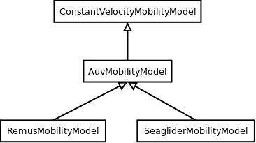
AUV’s mobility model classes overview
An ns3::AuvMobilityModel interface has been designed to give users a generic interface to access AUV’s navigation functions.
The AuvMobilityModel interface is implemented by the RemusMobilityModel and the GliderMobilityModel classes. The AUV’s mobility models organization it is shown in AUV’s mobility model classes overview.
Both models use a constant velocity movement, thus the AuvMobilityModel interface derives from the ConstantVelocityMobilityModel. The two classes hold the navigation parameters for the two different AUVs, like maximum pitch angles, maximum operating depth, maximum and minimum speed values. The Glider model holds also some extra parameters like maximum buoyancy values, and maximum and minimum glide slopes.
Both classes, RemusMobilityModel and GliderMobilityModel, handle also the AUV power consumption, utilizing the relative power models.
Has been modified the WaypointMobilityModel to let it use a generic underlying ConstantVelocityModel to validate the waypoints and, to keep trace of the node’s position. The default model is the classic ConstantVelocityModel but, for example in case of REMUS mobility model, the user can install the AUV mobility model into the waypoint model and then validating the waypoints against REMUS navigation constraints.
Energy models
The energy models have been designed as in the follows.
Use cases
The user will be able to:
- use a specific power profile for the acoustic modem
- use a specific energy model for the AUV
- trace the power consumption of AUV navigation, through AUV’s energy model
- trace the power consumption underwater acoustic communications, through acoustic modem power profile
We have integrated the Energy Model with the UAN module, to implement energy handling. We have implemented a specific energy model for the two AUV classes and, an energy source for Lithium batteries. This will be really useful for researchers to keep trace of the AUV operational life. We have implemented also an acoustic modem power profile, to keep trace of its power consumption. This can be used to compare protocols specific power performance. In order to use such power profile, the acoustic transducer physical layer has been modified to use the modem power profile. We have decoupled the physical layer from the transducer specific energy model, to let the users change the different energy models without changing the physical layer.
AUV energy models
Basing on the Device Energy Model interface, it has been implemented a specific energy model for the two AUV classes (REMUS and Seaglider). This models reproduce the AUV’s specific power consumption to give users accurate information. This model can be naturally used to evaluates the AUV operating life, as well as mission-related power consumption, etc. Have been developed two AUV energy models:
- GliderEnergyModel, computes the power consumption of the vehicle based on the current buoyancy value and vertical speed [5]
- RemusEnergyModel, computes the power consumption of the vehicle based on the current speed, as it is propelled by a brush-less electric motor
Note
TODO extend a little bit
AUV energy sources
Note
[TODO]
Acoustic modem energy model
Basing on the Device Energy Model interface, has been implemented a generic energy model for acoustic modem. The model allows to trace four modem’s power-states: Sleep, Idle, Receiving, Transmitting. The default parameters for the energy model are set to fit those of the WHOI  -modem. The class follows pretty closely the RadioEnergyModel class as the transducer behaviour is pretty close to that of a Wi-Fi radio.
The default power consumption values implemented into the model are as follows [6]:
| Modem State | Power Consumption |
| TX | 50 W |
| RX | 158 mW |
| Idle | 158 mW |
| Sleep | 5.8 mW |
UAN module energy modifications
The UAN module has been modified in order to utilize the implemented energy classes. Specifically, it has been modified the physical layer of the UAN module. It Has been implemented an UpdatePowerConsumption method that takes the modem’s state as parameter. It checks if an energy source is installed into the node and, in case, it then use the AcousticModemEnergyModel to update the power consumption with the current modem’s state. The modem power consumption’s update takes place whenever the modem changes its state.
A user should take into account that, if the power consumption handling is enabled (if the node has an energy source installed), all the communications processes will terminate whether the node depletes all the energy source.
Li-Ion batteries model
A generic Li-Ion battery model has been implemented based on [7] [8]. The model can be fitted to any type of Li-Ion battery simply changing the model’s parameters The default values are fitted for the Panasonic CGR18650DA Li-Ion Battery [9]. [TODO insert figure] As shown in figure the model approximates very well the Li-Ion cells. Regarding Seagliders, the batteries used into the AUV are Electrochem 3B36 Lithium / Sulfuryl Chloride cells [10]. Also with this cell type, the model seems to approximates the different discharge curves pretty well, as shown in the figure.
Note
should I insert the li-ion model deatils here? I think it is better to put them into an Energy-related chapter..
Scope and Limitations
The framework is designed to simulate AUV’s behaviour. We have modeled the navigation and power consumption behaviour of REMUS class and Seaglider AUVs. The communications stack, associated with the AUV, can be modified depending on simulation needs. Usually, the default underwater stack is being used, composed of an half duplex acoustic modem, an Aloha MAC protocol and a generic physical layer.
Regarding the AUV energy consumption, the user should be aware that the level of accuracy differs for the two classes:
- Seaglider, high level of accuracy, thanks to the availability of detailed information on AUV’s components and behaviour [5] [10]. Have been modeled both the navigation power consumption and the Li battery packs (according to [5]).
- REMUS, medium level of accuracy, due to the lack of publicly available information on AUV’s components. We have approximated the power consumption of the AUV’s motor with a linear behaviour and, the energy source uses an ideal model (BasicEnergySource) with a power capacity equal to that specified in [4].
Future Work
Some ideas could be :
- insert a data logging capability
- modify the framework to use sockets (enabling the possibility to use applications)
- introduce some more MAC protocols
- modify the physical layer to let it consider the Doppler spread (problematic in underwater environments)
- introduce OFDM modulations
References
| [1] | BINGHAM, D.; DRAKE, T.; HILL, A.; LOTT, R.; The Application of Autonomous Underwater Vehicle (AUV) Technology in the Oil Industry – Vision and Experiences, URL: http://www.fig.net/pub/fig_2002/Ts4-4/TS4_4_bingham_etal.pdf |
| [2] | AUVfest2008: Underwater mines; URL: http://oceanexplorer.noaa.gov/explorations/08auvfest/background/mines/mines.html |
| [3] | (1, 2, 3) Hydroinc Products; URL: http://www.hydroidinc.com/products.html |
| [4] | (1, 2, 3, 4) WHOI, Autonomous Underwater Vehicle, REMUS; URL: http://www.whoi.edu/page.do?pid=29856 |
| [5] | (1, 2, 3, 4, 5, 6) Eriksen, C.C., T.J. Osse, R.D. Light, T. Wen, T.W. Lehman, P.L. Sabin, J.W. Ballard, and A.M. Chiodi. Seaglider: A Long-Range Autonomous Underwater Vehicle for Oceanographic Research, IEEE Journal of Oceanic Engineering, 26, 4, October 2001. URL: http://ieeexplore.ieee.org/stamp/stamp.jsp?tp=&arnumber=972073&userType=inst |
| [6] | (1, 2) L. Freitag, M. Grund, I. Singh, J. Partan, P. Koski, K. Ball, and W. Hole, The whoi micro-modem: an acoustic communications and navigation system for multiple platforms, In Proc. IEEE OCEANS05 Conf, 2005. URL: http://ieeexplore.ieee.org/iel5/10918/34367/01639901.pdf |
| [7] | (1, 2) C. M. Shepherd, “Design of Primary and Secondary Cells - Part 3. Battery discharge equation,” U.S. Naval Research Laboratory, 1963 |
| [8] | (1, 2) Tremblay, O.; Dessaint, L.-A.; Dekkiche, A.-I., “A Generic Battery Model for the Dynamic Simulation of Hybrid Electric Vehicles,” Ecole de Technologie Superieure, Universite du Quebec, 2007 URL: http://ieeexplore.ieee.org/stamp/stamp.jsp?tp=&arnumber=4544139 |
| [9] | (1, 2, 3) Panasonic CGR18650DA Datasheet, URL: http://www.panasonic.com/industrial/includes/pdf/Panasonic_LiIon_CGR18650DA.pdf |
| [10] | (1, 2) Electrochem 3B36 Datasheet, URL: http://www.electrochem.com.cn/products/Primary/HighRate/CSC/3B36.pdf |
Usage
The main way that users who write simulation scripts will typically interact with the UAN Framework is through the helper API and through the publicly visible attributes of the model.
The helper API is defined in src/uan/helper/acoustic-modem-energy-model-helper.{cc,h} and in /src/uan/helper/...{cc,h}.
The example folder src/uan/examples/ contain some basic code that shows how to set up and use the models.
further examples can be found into the Unit tests in src/uan/test/...cc
Examples
Examples of the Framework’s usage can be found into the examples folder. There are mobility related examples and UAN related ones.
Mobility Model Examples
auv-energy-model:In this example we show the basic usage of an AUV energy model. Specifically, we show how to create a generic node, adding to it a basic energy source and consuming energy from the energy source. In this example we show the basic usage of an AUV energy model.
The Seaglider AUV power consumption depends on buoyancy and vertical speed values, so we simulate a 20 seconds movement at 0.3 m/s of vertical speed and 138g of buoyancy. Then a 20 seconds movement at 0.2 m/s of vertical speed and 138g of buoyancy and then a stop of 5 seconds.
The required energy will be drained by the model basing on the given buoyancy/speed values, from the energy source installed onto the node. We finally register a callback to the TotalEnergyConsumption traced value.
auv-mobility:In this example we show how to use the AuvMobilityHelper to install an AUV mobility model into a (set of) node. Then we make the AUV to submerge to a depth of 1000 meters. We then set a callback function called on reaching of the target depth. The callback then makes the AUV to emerge to water surface (0 meters). We set also a callback function called on reaching of the target depth. The emerge callback then, stops the AUV.
During the whole navigation process, the AUV’s position is tracked by the TracePos function and plotted into a Gnuplot graph.
waypoint-mobility:We show how to use the WaypointMobilityModel with a non-standard ConstantVelocityMobilityModel. We first create a waypoint model with an underlying RemusMobilityModel setting the mobility trace with two waypoints. We then create a waypoint model with an underlying GliderMobilityModel setting the waypoints separately with the AddWaypoint method. The AUV’s position is printed out every seconds.
UAN Examples
li-ion-energy-source- In this simple example, we show how to create and drain energy from a LiIonEnergySource. We make a series of discharge calls to the energy source class, with different current drain and durations, until all the energy is depleted from the cell (i.e. the voltage of the cell goes below the threshold level). Every 20 seconds we print out the actual cell voltage to verify that it follows the discharge curve [9]. At the end of the example it is verified that after the energy depletion call, the cell voltage is below the threshold voltage.
uan-energy-auv- This is a comprehensive example where all the project’s components are used. We setup two nodes, one fixed surface gateway equipped with an acoustic modem and a moving Seaglider AUV with an acoustic modem too. Using the waypoint mobility model with an underlying GliderMobilityModel, we make the glider descend to -1000 meters and then emerge to the water surface. The AUV sends a generic 17-bytes packet every 10 seconds during the navigation process. The gateway receives the packets and stores the total bytes amount. At the end of the simulation are shown the energy consumptions of the two nodes and the networking stats.
Helpers
In this section we give an overview of the available helpers and their behaviour.
AcousticModemEnergyModelHelper
This helper installs AcousticModemEnergyModel into UanNetDevice objects only. It requires an UanNetDevice and an EnergySource as input objects.
The helper creates an AcousticModemEnergyModel with default parameters and associate it with the given energy source. It configures an EnergyModelCallback and an EnergyDepletionCallback. The depletion callback can be configured as a parameter.
AuvGliderHelper
Installs into a node (or set of nodes) the Seaglider’s features:
- waypoint model with underlying glider mobility model
- glider energy model
- glider energy source
- micro modem energy model
The glider mobility model is the GliderMobilityModel with default parameters. The glider energy model is the GliderEnergyModel with default parameters.
Regarding the energy source, the Seaglider features two battery packs, one for motor power and one for digital-analog power. Each pack is composed of 12 (10V) and 42 (24V) lithium chloride DD-cell batteries, respectively [5]. The total power capacity is around 17.5 MJ (3.9 MJ + 13.6 MJ). In the original version of the Seaglider there was 18 + 63 D-cell with a total power capacity of 10MJ.
The packs design is as follows:
- 10V - 3 in-series string x 4 strings = 12 cells - typical capacity ~100 Ah
- 24V - 7 in-series-strings x 6 strings = 42 cells - typical capacity ~150 Ah
Battery cells are Electrochem 3B36, with 3.6 V nominal voltage and 30.0 Ah nominal capacity. The 10V battery pack is associated with the electronic devices, while the 24V one is associated with the pump motor.
The micro modem energy model is the MicroModemEnergyModel with default parameters.
AuvRemusHelper
Install into a node (or set of nodes) the REMUS features:
- waypoint model with REMUS mobility model validation
- REMUS energy model
- REMUS energy source
- micro modem energy model
The REMUS mobility model is the RemusMobilityModel with default parameters. The REMUS energy model is the RemusEnergyModel with default parameters.
Regarding the energy source, the REMUS features a rechargeable lithium ion battery pack rated 1.1 kWh @ 27 V (40 Ah) in operating conditions (specifications from [3] and Hydroinc European salesman). Since more detailed information about battery pack were not publicly available, the energy source used is a BasicEnergySource.
The micro modem energy model is the MicroModemEnergyModel with default parameters.
Attributes
Note
TODO
Tracing
Note
TODO
Logging
Note
TODO
Caveats
Note
TODO
Validation
This model has been tested with three UNIT test:
- auv-energy-model
- auv-mobility
- li-ion-energy-source
Auv Energy Model
Includes test cases for single packet energy consumption, energy depletion, Glider and REMUS energy consumption.
The unit test can be found in src/uan/test/auv-energy-model-test.cc.
The single packet energy consumption test do the following:
- creates a two node network, one surface gateway and one fixed node at -500 m of depth
- install the acoustic communication stack with energy consumption support into the nodes
- a packet is sent from the underwater node to the gateway
- it is verified that both, the gateway and the fixed node, have consumed the expected amount of energy from their sources
The energy depletion test do the following steps:
- create a node with an empty energy source
- try to send a packet
- verify that the energy depletion callback has been invoked
The Glider energy consumption test do the following:
- create a node with glider capabilities
- make the vehicle to move to a predetermined waypoint
- verify that the energy consumed for the navigation is correct, according to the glider specifications
The REMUS energy consumption test do the following:
- create a node with REMUS capabilities
- make the vehicle to move to a predetermined waypoint
- verify that the energy consumed for the navigation is correct, according to the REMUS specifications
Auv Mobility
Includes test cases for glider and REMUS mobility models.
The unit test can be found in src/uan/test/auv-mobility-test.cc.
- create a node with glider capabilities
- set a specified velocity vector and verify if the resulting buoyancy is the one that is supposed to be
- make the vehicle to submerge to a specified depth and verify if, at the end of the process the position is the one that is supposed to be
- make the vehicle to emerge to a specified depth and verify if, at the end of the process the position is the one that is supposed to be
- make the vehicle to navigate to a specified point, using direction, pitch and speed settings and, verify if at the end of the process the position is the one that is supposed to be
- make the vehicle to navigate to a specified point, using a velocity vector and, verify if at the end of the process the position is the one that is supposed to be
The REMUS mobility model test do the following: * create a node with glider capabilities * make the vehicle to submerge to a specified depth and verify if, at the end of the process the position is the one that is supposed to be * make the vehicle to emerge to a specified depth and verify if, at the end of the process the position is the one that is supposed to be * make the vehicle to navigate to a specified point, using direction, pitch and speed settings and, verify if at the end of the process the position is the one that is supposed to be * make the vehicle to navigate to a specified point, using a velocity vector and, verify if at the end of the process the position is the one that is supposed to be
WAVE models
WAVE is a system architecture for wireless-based vehicular communications, specified by the IEEE. This chapter documents available models for WAVE within ns-3. The focus is on the MAC layer and MAC extension layer defined by [ieee80211p] and [ieee1609dot4].
Model Description
WAVE is an overall system architecture for vehicular communications. The standards for specifying WAVE include a set of extensions to the IEEE 802.11 standard, found in IEEE Std 802.11p-2010 [ieee80211p], and the IEEE 1609 standard set, consisting of four documents: resource manager: IEEE 1609.1 [ieee1609dot1], security services: IEEE 1609.2 [ieee1609dot2], network and transport layer services: IEEE 1609.3 [ieee1609dot3], and multi-channel coordination: IEEE 1609.4 [ieee1609dot4]. Additionally, SAE standard J2735 [saej2735] describes a Dedicated Short Range Communications (DSRC) application message set that allows applications to transmit information using WAVE.
In ns-3, the focus of the wave module is on both the MAC layer and the
multi-channel coordination layer.
The key design aspect of 802.11p-compilant MAC layer is that they allow
communications outside the context of a basic service set (BSS).
The literature uses the acronym OCB to denote “outside the context
of a BSS”, and the class ns3::OcbWifiMac models this in ns-3.
This MAC does not require any association between devices (similar to an
adhoc WiFi MAC). Many management frames will not be used, but when used, the BSSID field
needs to be set to a wildcard BSSID value. Management information is
transmitted by what is called a vendor specific action (VSA) frame. With these
changes, the packet transmissions (for a moving vehicle) can be fast with
small delay in the MAC layer. Users can create IEEE802.11p-compliant device
(the object of the class ns3::WifiNetDevice associating with
ns3::OcbWifiMac) .
The key design aspect of the WAVE-compilant MAC layer (including 802.11p MAC layer and 1609.4 MAC extension layer) is that, based on OCB features, they provide devices with the capability of switching between control and service channels, using a single radio or using multiple radios. Therefore devices can communicate with others in single or multiple channels, which can support both safety related and non-safety related service for vehicular environments.
At the physical layer, the biggest difference is the use of the 5.9 GHz band with a channel bandwidth of 10 MHz. These physical layer changes can make the wireless signal relatively more stable, without degrading throughput too much (ranging from 3 Mbps to 27 Mbps).
The source code for the WAVE MAC models lives in the directory
src/wave.
For better modeling WAVE and VANET, the WAVE models for high layers (mainly [ieee1609dot3] ) are planned for a later patch.
Design
In ns-3, support for 802.11p involves the MAC and PHY layers.
To use an 802.11p NetDevice, ns3::Wifi80211pHelper is suggested.
In ns-3, support for WAVE involves the MAC, its MAC extension and PHY layers.
To use a WAVE NetDevice, ns3::WaveHelper is suggested.
MAC layer
The classes used to model the MAC layer are ns3::OrganizationIdentifier,
ns3::VendorSpecificActionHeader and ns3::OcbWifiMac.
The OrganizationIdentifier and VendorSpecificActionHeader are used to support the sending of a Vendor Specific Action frame.
OcbWifiMac is very similar to AdhocWifiMac, with some modifications. The ns-3 AdhocWifiMac class is implemented very close to the 802.11p OCB mode rather than a real 802.11 ad-hoc mode. The AdhocWifiMac has no BSS context that is defined in 802.11 standard, so it will not take time to send beacons and to authenticate, making its behavior similar to that of an OcbWifiMac.
- SetBssid, GetBssid, SetSsid, GetSsid
These methods are related to 802.11 BSS context, and are unused in the OCB context.
SetLinkUpCallback, SetLinkDownCallback
WAVE device can send packets directly, so the WiFi link is never down.
SendVsc, AddReceiveVscCallback
WAVE management information shall be sent by vendor specific action frames, sent by the upper layer 1609.4 standard as WSA (WAVE Service Advertisement) packets or other vendor specific information.
SendTimingAdvertisement (not implemented)
Although Timing Advertisement is very important and specifically defined in 802.11p standard, it is not useful in a simulation environment. Every node in ns-3 vehicular simulation is assumed to be already time synchronized (perhaps by GPS).
ConfigureEdca
This method will allow the user to set EDCA parameters of WAVE channels including CCH ans SCHs. And the OcbWifiMac itself also uses this method to configure default 802.11p EDCA parameters.
Wildcard BSSID
The Wildcard BSSID is set to “ff:ff:ff:ff:ff:ff”. As defined in IEEE 802.11-2007, a wildcard BSSID shall not be used in the BSSID field except for management frames of subtype probe request. But Adhoc mode of ns-3 simplifies this mechanism: when stations receive packets, they will be forwarded up to the higher layer, regardless of BSSID. This process is very close to OCB mode as defined in 802.11p-2010, in which stations use the wildcard BSSID to allow the higher layer of other stations to hear directly.
Enqueue, Receive
The most important methods are send and receive methods. According to the standard, we should filter the frames that are not permitted. Thus here we just identify the frames we care about; the other frames will be discarded.
MAC extension layer
Although 1609.4 is still in the MAC layer, the implementation
approach for ns-3 does not do much modification in the
source code of the wifi module. Instead, if some feature is related
to wifi MAC classes, then a relevant subclass is defined; if some
feature has no relation to wifi MAC classes, then a new class
will be defined. This approach was selected to be non-intrusive to the
ns-3 wifi module. All of these classes will be hosted in a ‘container’
class called ns3:: WaveNetDevice. This class is a subclass inherting
from ns3::NetDeivce, composed of the objects of
ns3::ChannelScheduler, ns3::ChannelManager,
ns3::ChannelCoordinator and ns3::VsaManager
classes to provide the features described in 1609.4 while still
containing the objects of ns3::OcbWifiMac and ns3::WifiPhy
classes. Moreover, ns3::OcbWifiMac class is further extended with
support for IEEE 1609.4 associating with ns3::HigherLayerTxVectorTag
and ns3::WaveMacLow. The main work of the WaveNetDevice is to create
objects, configure, check arguments and provide new APIs for multiple
channel operation as follows:
- AddMac, GetMac and GetMacs
Different fromns3::WifiNetDevice, the WAVE device will have multiple internal MAC entities rather than a single one. Each MAC entity is used to support each WAVE channel. Thus, when devices switch from the current channel to the next channel in different channel intervals, the packets in the internal queue will not be flushed and the current MAC entity will perform a suspend operation until woken up in next appropriate channel interval.
- AddPhy, GetPhy and GetPhys
Also in contrast tons3::WifiNetDevice, the WAVE device here can allow more than one PHY entity, which permits the use cases of of single-PHY devices or multiple-PHY devices.
- SetChannelScheduler and GetChannelScheduler
How to deal with multiple MAC entities and PHY entities to assign channel access for different requests from higher layer? IEEE 1609.4 [ieee1609dot4] does not seem to give a very clear and detailed mechanism, deferring to the implementor. In this model, the classns3::ChannelSchedulerprovides the API and delegates to the subclasses to implement the virtual methods. In the current implementation, the default assignment mechanism for channel access, calledns3::DefaultChannelScheduler, gives a simple answer that only deals with multiple channel operation in the context of a single-PHY device. If users define their own different assignment mechanisms such as in the context of two PHY entities, they can easily reuse models using AddPhy and SetChannelScheduler methods to import a new assignment mechanism.
- SetChannelManager and GetChannelManager
classns3::ChannelManageris a WAVE channel set which contains valid WAVE channel numbers. Moreover, the tx information in this channel set such as data rate and tx power level is used for transmitting management frames.
- SetVsaManager and GetVsaManager
classns3::VsaManageris used to deal with sending and receiving VSA frames. According to different request parameters from the higher layer, this class may transmit VSA frames repeatedly in the appropriate channel number and channel interval.
- SetChannelCoordinator and GetChannelCoordinator
classns3::ChannelCoordinatoris used to deal with channel coordination. The WAVE device can be aware of the channel interval at the current time or in the future. It can also notify listeners about incoming channel coordination events. Generally this class is used in the case of assigning alternating CCH and SCH access.
- StartSch and StopSch
In contrast to the basic 802.11p device that allow transmission packets immediately after the device is created, the WAVE device should assign channel access for sending packets. This method will call classns3::ChannelSchedulerto assign radio resources for the relevant channel.
- ChangeAddress
The WAVE device can support a change of address after devices are already initialized, which will cause all of MAC entities reset their status.
- CancelTx
The WAVE device can support a request to cancel all transmissions associated with the particular category and channel number, which will reset the particular interval queue and drop all of the queued packets in this queue.
- RegisterTxProfile and DeleteTxProfile
After channel access is assigned, we still cannot send IP-based (or other protocol) packets by the Send () method. A tx profile should be registered to specify tx parameters before transmission.
- StartVsa, StopVsa and SetWaveVsaCallback
These methods will call an object from classns3::VsaManagerto send and receive VSA frames. Generally these methods are used by IEEE 1609.3 for WSA management information.
- SendX
After channel access is assigned, we can send WSMP (or other protocol) packets via the SendX () method. We should specify the tx parameters for each packet, e.g. the channel number for transmit.
- Send and SetReceiveCallback
This method is the abstract method defined in the parent classns3::NetDevice, defined to allow the sending of IP-based packets. The channel access should be already assigned and tx profile should be registered, otherwise incoming packets from the higher layer will be discarded. No matter whether packets are sent by Send method or SendX method, the received packets will be only be delivered to the higher layer by the registered ReceiveCallback.
- other methods from its parent class
ns3::NetDevice
These methods are implemented very similar to the code inns3::WifiNetDevice.
In the above numbered list, we can categorize the methods into three types: the first type, from 1 to 6 and also 14, is the configuration for modeling and creating a WAVE device; the second type, from 7 to 11, is the management plane of the standard; and the third type, 12 and 13, is the data plane of the standard.
Channel coordination
The class ns3::ChannelCoordinator defines the CCH Interval, SCH Interval and GuardInteval. Users can be aware of which interval the current time or
future time will be in. If channel access mode is assigned to
alternating CCH and SCH access,
channel interval events will be notified repeatedly for class
ns3::ChannelCoordinator to switch channels. Current default values are
for CCHI with 50ms interval, SCHI with 50ms interval, and GuardI with 4ms interval. Users can change these values by configuring the class attributes.
Channel routing
Channel routing service means different transmission approaches for WSMP data,
IP datagram and management information.
For WSMP data, the SendX () method implements the service primitive
MA-UNITDATAX, and users can
set transmission parameters for each individual packet. The parameters include
channel number, priority,
data rate and tx power level (expiration time is not supported now).
For IP datagrams, the Send () method is a virtual method from ns3::NetDevice that implements the service primitive MA-UNITDATA.
Users should insert QoS tags into packets themselves if they want to use QoS.
Moreover, a tx profile should be registered
before the Send method is called for transmit; the profile contains SCH number, data rate, power level and adaptable mode.
For management information, StartVsa method implements the service primitive
MLMEX-VSA. The tx information is already configured
in ns3::ChannelManager, including data rate, power level and adaptable mode.
Channel access assignment
The channel access assignment is done by class ns3::ChannelScheduler to assign ContinuousAccess, ExtendedAccess
and AlternatingAccess. Besides that, immediate access is achieved by enabling
the “immediate” parameter, in which case
the request channel will be switched to immediately. However this class is a
virtual parent class. The current module provides a
subclass ns3::DefaultChannelScheduler to assign channel access in the context of a single-PHY device. In this subclass, if the channel
access is already assigned for another request, the next coming request will
fail until the previous channel access is released.
Users can implement different assignment mechanisms to deal with multiple MAC entities and multiple PHY entities by
inheriting from parent class ns3::ChannelScheduler.
An important point is that channel access should be assigned before sending
routing packets, otherwise the packets will be discard.
Vendor Specific Action frames
When users want to send VSA repeatedly by calling WaveNetDevice::StartVsa, VSA will be sent repeatedly by
ns3::VsaManager. It is worth noting that if the peer MAC address is a unicast address, the VSA can only
be transmitted once even there is a repeat request. The tx parameters for VSA management frames can be obtained from the ns3::ChannelManager.
User priority and Multi-channel synchronization
Since wifi module has already implemented a QoS mechanism, the wave module reuses the mechanism; VSA frames will be assigned the default value with the highest AC according to the standard. Multiple-channel synchronization is very important in practice for devices without a local timing source. However, in simulation, every node is supposed to have the same system clock, which could be provided by GPS devices in a real environment, so this feature is not modelled in ns-3. During the guard interval, the device can only be in receive state, except for the switch state when the device does channel switching operation.
PHY layer
No modification or extension is made to the ns-3 PHY layer corresponding to this model. In the 802.11p standard, the PHY layer wireless technology is still 80211a OFDM with a 10MHz channel width, so Wifi80211pHelper will only allow the user to set the standard to WIFI_PHY_STANDARD_80211_10MHZ or WIFI_PHY_STANDARD_80211_20MHZ, while WaveHelper will only support WIFI_PHY_STANDARD_80211_10MHZ. The maximum station transmit power and maximum permitted EIRP defined in 802.11p is larger than that of WiFi, so transmit range can normally become longer than the usual WiFi. However, this feature will not be implemented. Users who want to obtain longer range should configure attributes “TxPowerStart”, “TxPowerEnd” and “TxPowerLevels” of the YansWifiPhy class by themselves.
Scope and Limitations
- Does the model involve vehicular mobility of some sort?
Vehicular networks involve not only communication protocols, but
also a communication environment including vehicular mobility and
propagation loss models. Because of specific features of the latter,
the protocols need to change. The MAC layer model in this project just
adapts MAC changes to vehicular environment. However this model
does not involve any vehicular mobility with time limit. While users
should understand that vehicular mobility is out of scope for the
current WAVE module, they can use any mobility model in ns-3. For
example, users may use a ns3::RandomWaypointMobilityModel (RWP)
for node mobilty or may generate ns-2-style playback files using
other third-party tools and then playback those mobility traces
using ns3::Ns2MobilityHelper.
- Does this model use different propagation models?
Referring to the first issue, some more realistic propagation loss
models for vehicualr environment are suggested and welcome. Some
existing propagation los models in ns-3 are also suitable.
Normally, users can use Friis, Two-Ray Ground, and Nakagami models.
The ns3::VanetRoutingExample example defaults to Two-Ray
Ground propagation loss with no additional fading, although adding
stochastic Nakagami-m fading is parametrically supported.
- Are there any vehicular application models to drive the code?
About vehicular application models, SAE J2375 depends on WAVE
architecture and is an application message set in US. Cooperative Awareness
Messages (CAM) and Decentralized Environment Notification Messages (DENM) can
be sent Europe between network and application layer, and is
very close to being an application model. The BSM in J2375 [saej2735] and CAM
send alert messages that every vehicle node will sent periodically about
its status information to cooperate with others. The
ns3::VanetRoutingExample example sets up a network of (vehicular)
nodes that each broadcast BSMs at regular intervals and may additionally
attempt to route non-BSM data through the network using select IP-based
routing protocols.
- Why are there two kinds of NetDevice helpers?
The current module provides two helpers to create two kinds of NetDevice.
The first is an object of WifiNetDevice (802.11p device) which mainly
contains class ns3::OcbWifiMac to enable OCB mode. The second
is an object of WaveNetDevice (WAVE device) which contains additional
classes ns3::ChannelScheduler, ns3::ChannelManager,
ns3::ChannelCoordinator and ns3::VsaManager to support
multi-channel operation mode. The reason to provide a special 802.11p
device helper is that, considering the fact that many researchers are
interested in routing protocols or other aspects of vehicular environment in
a single channel context, they need neither multi-channel operation nor
WAVE architectures.
Besides that, the European standard may also reuse an 802.11p device in an
modified ITS-G5 implementation (maybe called ItsG5NetDevice). Hence,
the model supports configuration of both types of devices.
References
| [ieee80211p] | (1, 2) IEEE Std 802.11p-2010 “IEEE Standard for Information technology– Local and metropolitan area networks– Specific requirements– Part 11: Wireless LAN Medium Access Control (MAC) and Physical Layer (PHY) Specifications Amendment 6: Wireless Access in Vehicular Environments” |
| [ieee1609dot1] | IEEE Std 1609.1-2010 “IEEE Standard for Wireless Access in Vehicular Environments (WAVE) - Resource Manager, 2010” |
| [ieee1609dot2] | IEEE Std 1609.2-2010 “IEEE Standard for Wireless Access in Vehicular Environments (WAVE) - Security Services for Applications and Management Messages, 2010” |
| [ieee1609dot3] | (1, 2) IEEE Std 1609.3-2010 “IEEE Standard for Wireless Access in Vehicular Environments (WAVE) - Networking Services, 2010” |
| [ieee1609dot4] | (1, 2, 3) IEEE Std 1609.4-2010 “IEEE Standard for Wireless Access in Vehicular Environments (WAVE) - Multi-Channel Operation, 2010” |
| [saej2735] | SAE Std J2735 “J2735 dedicated short range communications (DSRC) message set dictionary. 2009” |
Usage
Helpers
The helpers include a) lower-level MAC and PHY channel helpers and b) higher-level application helpers that handle the sending and receiving of the Basic Safety Message (BSM).
The lower-level helpers include ns3::YansWavePhyHelper, ns3::NqosWaveMacHelper, ns3::QosWaveMacHelper,
ns3::Wifi80211pHelper and ns3::WaveHelper.
Wifi80211pHelper is used to create 802.11p devices that follow the 802.11p-2010 standard. WaveHelper is used to create WAVE devices that follow both 802.11p-2010 and 1609.4-2010 standards which are the MAC and PHY layers of the WAVE architecture.
The relation of ns3::NqosWaveMacHelper, ns3::QosWaveMacHelper and
ns3::Wifi80211pHelper is described as below:
WifiHelper ------------use--------------> WifiMacHelper
^ ^ ^
| | |
| | |
inherit inherit inherit
| | |
Wifi80211pHelper ------use-----> QosWaveMacHelper or NqosWaveHelper
From the above diagram, there are two Mac helper classes that both inherit from the WifiMacHelper; when the WAVE module was originally written, there were specialized versions (QoS and Nqos) of WifiMacHelper that have since been removed from the Wifi codebase, but the distinction remains in the WAVE helpers. The functions of WiFi 802.11p device can be achieved by WaveNetDevice’s ContinuousAccess assignment, Wifi80211pHelper is recommended if there is no need for multiple channel operation. Usage is as follows:
NodeContainer nodes;
NetDeviceContainer devices;
nodes.Create (2);
YansWifiPhyHelper wifiPhy = YansWifiPhyHelper::Default ();
YansWifiChannelHelper wifiChannel = YansWifiChannelHelper::Default ();
wifiPhy.SetChannel (wifiChannel.Create ());
NqosWave80211pMacHelper wifi80211pMac = NqosWaveMacHelper::Default();
Wifi80211pHelper 80211pHelper = Wifi80211pHelper::Default ();
devices = 80211pHelper.Install (wifiPhy, wifi80211pMac, nodes);
The relation of ns3::YansWavePhyHelper, ns3::QosWaveMacHelper and ns3::WaveHelper
is described as below:
WifiMacHelper
^
|
inherit
|
WaveHelper -------- only use --------> QosWaveMacHelper
From the above diagram, WaveHelper is not the subclass of WifiHelper and should only use QosWaveMacHelper because WAVE MAC layer is based on QoS mechanism. But the WaveHelper is recommended if there is a need for multiple channel operation. Usage is as follows:
NodeContainer nodes;
NetDeviceContainer devices;
nodes.Create (2);
YansWifiChannelHelper wifiChannel = YansWifiChannelHelper::Default ();
YansWavePhyHelper wavePhy = YansWavePhyHelper::Default ();
wavePhy.SetChannel (wifiChannel.Create ());
QosWaveMacHelper waveMac = QosWaveMacHelper::Default ();
WaveHelper waveHelper = WaveHelper::Default ();
devices = waveHelper.Install (wavePhy, waveMac, nodes);
The higher-level helpers include ns3::WaveBsmStats and ns3::WaveBsmHelper.
WaveBsmStats is used to collect and manage statistics, such as packet and byte counts and Packet Delivery Ratio (PDR), regarding the sending and receiving of WAVE BSM packets. WaveBsmHelper is used by applications that wish to send and receive BSMs.
The relation of ns3::WaveBsmHelper and WaveBsmStats is described
below:
<Your Vanet Routing Application> ----use----> WaveBsmHelper ----use----> WaveBsmStats
From <Your Vanet Routing Application>, usage is as follows:
// declare WAVE BSM helper instance WaveBsmHelper m_waveBsmHelper;
// the following are passed to the WaveBsmHelpe::Install() // method, and they are thus assumed to be created and // initialized themselves, based on the user’s // simulation setup criteria. // container of network node NodeContainer m_adhocTxNodes; // (transmitting) devices (1 per node) NetDeviceContainer m_adhocTxDevices; // IPv4 interfaces (1 per device) Ipv4InterfaceContainer m_adhocTxInterfaces; // total simulation time (in seconds) double m_TotalSimTime; // WAVE BSM broadcast interval. E.g., 100ms = 0.1 seconds double m_waveInterval; // seconds // time-synchronization accuracy of GPS devices. E.g., +/- 40ns double m_gpsAccuracyNs; // array of distances (m) at which safety PDR shall be determined, // e.g. 50m, 100m, 200m, 300m, 400m, 500m, 600m, 800m, 1000m, and 1500m std::vector <double> m_txSafetyRanges; // used to get consistent random numbers across scenarios int64_t m_streamIndex;
- m_waveBsmHelper.Install (m_adhocTxNodes,
- m_adhocTxDevices, m_adhocTxInterfaces, Seconds(m_TotalSimTime), m_wavePacketSize, Seconds(m_waveInterval), // convert GPS accuracy, in ns, to Time Seconds(m_gpsAccuracyNs / 1000000.0), m_txSafetyRanges);
// fix random number streams m_streamIndex += m_waveBsmHelper.AssignStreams (m_streamIndex);
Example usages of BSM statistics are as follows:
// Get the cumulative PDR of the first safety Tx range (i.e, 50m in the // m_txSafetyRanges example above). double bsm_pdr1 = m_waveBsmHelper.GetWaveBsmStats ()->GetBsmPdr (1);
// total WAVE BSM bytes sent uint32_t cumulativeWaveBsmBytes = m_waveBsmHelper.GetWaveBsmStats ()->GetTxByteCount ();
// get number of WAVE BSM packets sent int wavePktsSent = m_waveBsmHelper.GetWaveBsmStats ()->GetTxPktCount ();
// get number of WAVE BSM packets received int wavePktsReceived = m_waveBsmHelper.GetWaveBsmStats ()->GetRxPktCount ();
// reset count of WAVE BSM packets received m_waveBsmHelper.GetWaveBsmStats ()->SetRxPktCount (0);
// reset count of WAVE BSM packets sent m_waveBsmHelper.GetWaveBsmStats ()->SetTxPktCount (0);
// indicate that a node (nodeId) is moving. (set to 0 to “stop” node) WaveBsmHelper::GetNodesMoving()[nodeId] = 1;
APIs
MAC layer
The 802.11p device can allow the upper layer to send different information over Vendor Specific Action management frames by using different OrganizationIdentifier fields to identify differences.
- create some Node objects and WifiNetDevice objects, e.g. one sender and one receiver.
- receiver defines an OrganizationIdentifier
uint8_t oi_bytes[5] = {0x00, 0x50, 0xC2, 0x4A, 0x40}; OrganizationIdentifier oi(oi_bytes,5);
- receiver defines a Callback for the defined OrganizationIdentifier
VscCallback vsccall = MakeCallback (&VsaExample::GetWsaAndOi, this);
- receiver registers this identifier and function
Ptr<WifiNetDevice> device1 = DynamicCast<WifiNetDevice>(nodes.Get (i)->GetDevice (0)); Ptr<OcbWifiMac> ocb1 = DynamicCast<OcbWifiMac>(device->GetMac ()); ocb1->AddReceiveVscCallback (oi, vsccall);
- sender transmits management information over VSA frames
Ptr<Packet> vsc = Create<Packet> (); ocb2->SendVsc (vsc, Mac48Address::GetBroadcast (), m_16093oi);
- then registered callbacks in the receiver will be called.
MAC extension layer
The WAVE devices allow the upper layer to route packets in different control approaches. However dedicated APIs and invocation sequences should be followed; otherwise, the packets may be discarded by devices.
- create some Node objects and WaveNetDevice objects by helpers, e.g. one sender and one receiver.
- receiver registers the receive callback if WSMP and IP-based packets are supposed to be received.
// the class ``ns3::WaveNetDeviceExample``here will has a receive method "Receive" to be registered. receiver->SetReceiveCallback (MakeCallback (&WaveNetDeviceExample::Receive, this));
- receiver registers the receive callback if WSA frames are supposed to be received.
// the class ``ns3::WaveNetDeviceExample``here will has a receive method "ReceiveVsa" to be registered. receiver->SetWaveVsaCallback (MakeCallback (&WaveNetDeviceExample::ReceiveVsa, this));
- sender and receiver assign channel access by StartSch method.
// in this case that alternating access with non-immediate mode is assigned for sender and receiver devices. const SchInfo schInfo = SchInfo (SCH1, false, EXTENDED_ALTERNATING); Simulator::Schedule (Seconds (0.0), &WaveNetDevice::StartSch, sender, schInfo); Simulator::Schedule (Seconds (0.0), &WaveNetDevice::StartSch, receiver, schInfo);or
// in this case that continuous access with immediate mode is assigned for sender and receiver devices. const SchInfo schInfo = SchInfo (SCH1, true, EXTENDED_CONTINUOUS); Simulator::Schedule (Seconds (0.0), &WaveNetDevice::StartSch, sender, schInfo); Simulator::Schedule (Seconds (0.0), &WaveNetDevice::StartSch, receiver, schInfo)or
// in this case that extended access with non-immediate mode is assigned for sender and receiver devices. const SchInfo schInfo = SchInfo (SCH1, false, 100); Simulator::Schedule (Seconds (0.0), &WaveNetDevice::StartSch, sender, schInfo); Simulator::Schedule (Seconds (0.0), &WaveNetDevice::StartSch, receiver, schInfo)
- sender registers a tx profile if IP-based packets are planned to be transmitted
// the IP-based packets will be transmitted in SCH1 with 6Mbps and 4 txPowerLevel with adaptable mode. const TxProfile txProfile = TxProfile (SCH1, true, 4, WifiMode("OfdmRate6MbpsBW10MHz")); Simulator::Schedule (Seconds (2.0), &WaveNetDevice::RegisterTxProfile, sender, txProfile);
- sender transmits WSMP packets by SendX method.
// the data rate and txPowerLevel is controlled by the high layer which are 6Mbps and 0 level here. const TxInfo txInfo = TxInfo (CCH, 7, WifiMode("OfdmRate6MbpsBW10MHz"), 0); // this packet will contain WSMP header when IEEE 1609.3 model is implemented const static uint16_t WSMP_PROT_NUMBER = 0x88DC; Ptr<Packet> wsaPacket = Create<Packet> (100); const Address dest = receiver->GetAddress (); Simulator::Schedule (Seconds (2.0), &WaveNetDevice::SendX, sender, wsaPacket, dest, WSMP_PROT_NUMBER, txInfo);or
// the data rate and txPowerLevel is controlled by the MAC layer which are decided by WifiRemoteStationManager const TxInfo txInfo = TxInfo (CCH, 7, WifiMode(), 8); // this packet will contain WSMP header when IEEE 1609.3 model is implemented const static uint16_t WSMP_PROT_NUMBER = 0x88DC; Ptr<Packet> wsaPacket = Create<Packet> (100); const Address dest = receiver->GetAddress (); Simulator::Schedule (Seconds (2.0), &WaveNetDevice::SendX, sender, wsaPacket, dest, WSMP_PROT_NUMBER, txInfo);
- sender transmits IP-based packets by Send method.
const static uint16_t IPv6_PROT_NUMBER = 0x86DD; Ptr<Packet> packet = Create<Packet> (100); const Address dest = receiver->GetAddress (); Simulator::Schedule (Seconds (2.0), &WaveNetDevice::Send, sender, packet, dest, IPv6_PROT_NUMBER);
- send transmits WSA frames repeatedly by StartVsa method.
// this packet will contain WSA management information when IEEE 1609.3 model is implemented Ptr<Packet> wsaPacket = Create<Packet> (100); Mac48Address dest = Mac48Address::GetBroadcast (); const VsaInfo vsaInfo = VsaInfo (dest, OrganizationIdentifier (), 0, wsaPacket, SCH1, 100, VSA_TRANSMIT_IN_BOTHI); Simulator::Schedule (Seconds (2.0), &WaveNetDevice::StartVsa, sender, vsaInfo);
- sender stops WSA frames repeatedly transmit by StopVsa method.
Simulator::Schedule (Seconds (3.0), &WaveNetDevice::StopVsa, sender, SCH1);
- sender and receiver release assigned channel access by StopSch method.
Simulator::Schedule (Seconds (4.0), &WaveNetDevice::StopSch, sender, SCH1); Simulator::Schedule (Seconds (4.0), &WaveNetDevice::StopSch, receiver, SCH1);
- sender or receiver changes current MAC address by ChangeAddress method.
Address newAddress = Mac48Address::Allocate (); Simulator::Schedule (Seconds (4.0), &WaveNetDevice::ChangeAddress, sender, newAddress);
- sender cancels all transmissions with the particular category and channel number by CancelTx method.
Simulator::Schedule (Seconds (4.0), &WaveNetDevice::CancelTx, sender, CCH, AC_BE);
For transmitting and receiving these packets successfully, the normal and appropriate invocation procedures should be performed.
(a) For WSMP, channel access should be assigned for transmit and receive. The channel access release operation may be optional if there is no need for transmission in another channel.
StartSch -------------> SendX / ReceiveCallback --------------> StopSch
(b) For IP, a tx profile should be registered before transmit and receive operations. The delete operation of tx profile may be optional if there is no need for transmission with other tx parameters. The channel access assignment and release optional usage is the same with WSMP here.
StartSch -------------> RegisterTxProfile ----------> Send / ReceiveCallback --------------> DeleteTxProfile -------------> StopSch
(c) For WSA, StartVsa is called to transmit while StopVsa is an optional operation for canceling repeat transmit. The channel access assignment and release optional usage is also the same with WSMP here. To receive VSA, WaveVsaCallback should be registered; otherwise, the received VSA frames will be discard by the MAC extension layer and not delivered to the higher layer.
StartSch -------------> StartVsa / WaveVsaCallback --------------> StopVsa ---------------> StopSch
(d) Here an important point is that if the higher layer wants to transmit these packets in a control channel (the channel 178), there will be no need to request for CCH by the StartSch method, which means that StartSch can be optional or should be avoided here. The reason is that the default continuous CCH access has been assigned automatically after WAVE devices are created and initialized. Therefore, if calling StartSch and StopSch method with CCH as a parameter, the request will be discarded by devices and the method will return false to indicate failure.
Attributes
The channel interval duration’s default value is defined in the standard.
However, the current implementation allows users to configure these
attributes with other values. These attributes are included in the class
ns3::ChannelCoodinator with config paths shown in the below. The method
IsValidConfig is suggested to test whether new configuration follows the
standard.
/NodeList/[i]/DeviceList/[i]/$ns3::WaveNetDevice/ChannelCoordinator/$ns3::ChannelCoordinator/CchInterval
/NodeList/[i]/DeviceList/[i]/$ns3::WaveNetDevice/ChannelCoordinator/$ns3::ChannelCoordinator/SchInterval
/NodeList/[i]/DeviceList/[i]/$ns3::WaveNetDevice/ChannelCoordinator/$ns3::ChannelCoordinator/GuardInterval
The ns3::WaveNetDevice is a wrapper class that contains those classes to support for multiple channel
operation. To set or get the pointers of those objects, users can also
use them by config paths shown in the below.
/NodeList/[i]/DeviceList/[i]/$ns3::WaveNetDevice/Mtu
/NodeList/[i]/DeviceList/[i]/$ns3::WaveNetDevice/Channel
/NodeList/[i]/DeviceList/[i]/$ns3::WaveNetDevice/PhyEntities
/NodeList/[i]/DeviceList/[i]/$ns3::WaveNetDevice/MacEntities
/NodeList/[i]/DeviceList/[i]/$ns3::WaveNetDevice/ChannelScheduler
/NodeList/[i]/DeviceList/[i]/$ns3::WaveNetDevice/ChannelManager
/NodeList/[i]/DeviceList/[i]/$ns3::WaveNetDevice/ChannelCoordinator
/NodeList/[i]/DeviceList/[i]/$ns3::WaveNetDevice/VsaManager
Output
For the 802.11p device, current classes provide output of the same type as WiFi devices; namely, ASCII and pcap traces, and logging output. The 802.11p logging components can be enabled globally via the call to
Wifi80211pHelper::EnableLogComponents ();
For the WAVE device, current classes provide output of the same type as WiFi devices; namely, ASCII and pcap traces, and logging output. The WAVE logging components can be enabled globally via the call to
WaveHelper::EnableLogComponents ();
Advanced Usage
Advanced WaveHelper configuration
If users can make sure in which channel this WAVE device will work, they can set specific channel numbers to save resources of unused channels . Usage is as follows:
// in this case, the MAC entities for SCH2 to SCH6 will not be created
WaveHelper helper = WaveHelper::Default ();
uint32_t channels[] = {CCH, SCH1};
std::vector<uint32_t> channelsVector (channels, channels + 2);
helper.CreateMacForChannel (channelsVector);
If users can create other channel access assignment mechanism, e.g. in the context of more PHY entities, which may be called “ns3::AnotherScheduler”, they can use this helper to create WAVE devices with new assignment mechanisms. Usage is as follows:
WaveHelper helper = WaveHelper::Default ();
helper.helper.CreateMacForChannel (ChannelManager::GetWaveChannels ()); // create all 7 MAC entities for WAVE
helper.CreatePhys (2); // or other number which should be less than 7
helper.SetChannelScheduler ("ns3::AnotherScheduler"); // The AnotherScheduler should be implemented by users.
helper.SetRemoteStationManager ("ns3::ConstantRateWifiManager"); // or other rate control algorithms
Examples
A basic example exists called wave-simple-80211p.cc.
This example shows basic construction of an 802.11p node. Two nodes
are constructed with 802.11p devices, and by default, one node sends a single
packet to another node (the number of packets and interval between
them can be configured by command-line arguments). The example shows
typical usage of the helper classes for this mode of WiFi.
Another example exists called wave-simple-device.cc. This
example shows how to create WAVE devices by helpers and the routing service
for different packets.
After WAVE devices are configured and created by helpers, these packets are
transmitted in different approaches.
Another example exists called vanet-routing-compare.cc. This
example shows how to create mobility nodes in a VANET scenario and
send Basic Safety Message (BSM) packets are regular intervals and/or
additional data traffic to be routed between nodes. BSMs are transmitted
assuming the WAVE Short Message Protocol (WSMP), whereas non-BSM data
packets are relayed by using one of several different IP-based routing
protocols (e.g., AODV, OLSR, DSDV, or DSR).
Troubleshooting
To be defined.
Validation
A test suite named wifi-80211p-ocb is defined. This test
case consists of a stationary node and a mobile node. The mobile
node moves towards the stationary mode, and time points are checked
at which time the physical layer starts to receive packets (and
whether the MAC becomes associated, if applicable). The same physical
experiment is repeated for normal WiFi NetDevices in AP/STA mode, in
Adhoc mode, and the new OCB mode.
Another test suite named wave-mac-extension is defined. This test suite
has four test cases, including channel-coordination, channel-routing,
channel-access and annex-c. The first case is to test channel
coordination
feature. The second case is to test channel routing for three types of packets.
The third case is to test four channel access assignments. And the fourth case
is to test the implemented feature described in the Annex C of the standard.
It is worth noting that the channel-routing and channel-access test
cases are both in the context of single-PHY device, which depends on the
default channel
access assignment mechanism ns3:DefaultChannelScheduler, thus they may not
be suitable for testing when other channel access assignment mechanisms are
used. Although they are test cases, they are also good examples to show
usage.
The ns3::VanetRoutingExample example was studied using mobility trace
files in the Raleigh, NC USA area generated using Simulation for Urban
Mobility (SUMO). Three environments were studied: a) an open highway
scenario, b) a residential neighborhood scenario, and c) and urban downtown
scenario. For each environment, a constant number of 50-750 vehicles was
maintained for 2000 simulation seconds (> 30 minutes). The mobility trace
file were played back using ns3::Ns2MobilityHelper. All vehicular nodes
transmitted a 200-byte BSM at 10 Hz and the PDR was determined for
transmission ranges of 50-1500m. No additional non-BSM data was injected /
routed through the network. The default propagation loss model used
was Two-Ray Ground. Different fading / shadowing models were evaluated,
including a) no fading, b) stochastic Nakagami-m fading, and c) an
obstacle shadowing model (to be contributed to ns-3). 30 trials of each
scenario were run in the North Carolina State University (NCSU) High
Performance Computing (HPC) center, with each trial requiring from
8 hours to 6 days of CPU time to complete. Preliminary results were
presented at the PhD Forum, 22nd IEEE International Conference on
Network Protocols (ICNP), October 24, 2014, Research Triangle Park, NC.
See: http://www4.ncsu.edu/~scarpen/Research_files/Final-PHD_Forum_SE_Carpenter_2014.pdf
Wi-Fi Module
Design Documentation
ns-3 nodes can contain a collection of NetDevice objects, much like an actual computer contains separate interface cards for Ethernet, Wifi, Bluetooth, etc. This chapter describes the ns-3 WifiNetDevice and related models. By adding WifiNetDevice objects to ns-3 nodes, one can create models of 802.11-based infrastructure and ad hoc networks.
Overview of the model
The WifiNetDevice models a wireless network interface controller based on the IEEE 802.11 standard [ieee80211]. We will go into more detail below but in brief, ns-3 provides models for these aspects of 802.11:
- basic 802.11 DCF with infrastructure and adhoc modes
- 802.11a, 802.11b, 802.11g, 802.11n (both 2.4 and 5 GHz bands), 802.11ac and 802.11ax (2.4, 5 and 6 GHz bands) physical layers
- MSDU aggregation and MPDU aggregation extensions of 802.11n, and both can be combined together (two-level aggregation)
- 802.11ax DL OFDMA and UL OFDMA (including support for the MU EDCA Parameter Set)
- QoS-based EDCA and queueing extensions of 802.11e
- the ability to use different propagation loss models and propagation delay models, please see the chapter on Propagation for more detail
- packet error models and frame detection models that have been validated against link simulations and other references
- various rate control algorithms including Aarf, Arf, Cara, Onoe, Rraa, ConstantRate, Minstrel and Minstrel-HT
- 802.11s (mesh), described in another chapter
- 802.11p and WAVE (vehicular), described in another chapter
The set of 802.11 models provided in ns-3 attempts to provide an accurate MAC-level implementation of the 802.11 specification and to provide a packet-level abstraction of the PHY-level for different PHYs, corresponding to 802.11a/b/e/g/n/ac/ax specifications.
In ns-3, nodes can have multiple WifiNetDevices on separate channels, and the WifiNetDevice can coexist with other device types. With the use of the SpectrumWifiPhy framework, one can also build scenarios involving cross-channel interference or multiple wireless technologies on a single channel.
The source code for the WifiNetDevice and its models lives in the directory
src/wifi.
The implementation is modular and provides roughly three sublayers of models:
- the PHY layer models: they model amendment-specific and common PHY layer operations and functions.
- the so-called MAC low models: they model functions such as medium access (DCF and EDCA), frame protection (RTS/CTS) and acknowledgment (ACK/BlockAck). In ns-3, the lower-level MAC is comprised of a Frame Exchange Manager hierarchy, a Channel Access Manager and a MAC middle entity.
- the so-called MAC high models: they implement non-time-critical processes in Wifi such as the MAC-level beacon generation, probing, and association state machines, and a set of Rate control algorithms. In the literature, this sublayer is sometimes called the upper MAC and consists of more software-oriented implementations vs. time-critical hardware implementations.
Next, we provide an design overview of each layer, shown in Figure WifiNetDevice architecture.
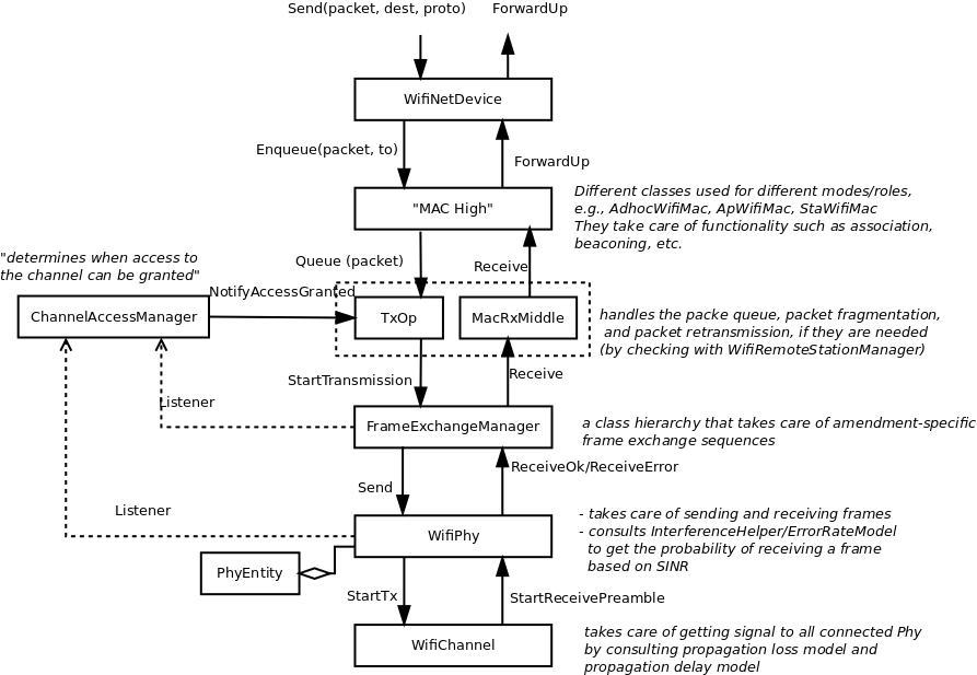
WifiNetDevice architecture
MAC high models
There are presently three MAC high models that provide for the three
(non-mesh; the mesh equivalent, which is a sibling of these with common
parent ns3::RegularWifiMac, is not discussed here) Wi-Fi topological
elements - Access Point (AP) (ns3::ApWifiMac),
non-AP Station (STA) (ns3::StaWifiMac), and STA in an Independent
Basic Service Set (IBSS) - also commonly referred to as an ad hoc
network (ns3::AdhocWifiMac).
The simplest of these is ns3::AdhocWifiMac, which implements a
Wi-Fi MAC that does not perform any kind of beacon generation,
probing, or association. The ns3::StaWifiMac class implements
an active probing and association state machine that handles automatic
re-association whenever too many beacons are missed. Finally,
ns3::ApWifiMac implements an AP that generates periodic
beacons, and that accepts every attempt to associate.
These three MAC high models share a common parent in
ns3::RegularWifiMac, which exposes, among other MAC
configuration, an attribute QosSupported that allows
configuration of 802.11e/WMM-style QoS support.
There are also several rate control algorithms that can be used by the MAC low layer. A complete list of available rate control algorithms is provided in a separate section.
MAC low layer
The MAC low layer is split into three main components:
ns3::FrameExchangeManagera class hierarchy which implement the frame exchange sequences introduced by the supported IEEE 802.11 amendments. It also handles frame aggregation, frame retransmissions, protection and acknowledgment.ns3::ChannelAccessManagerwhich implements the DCF and EDCAF functions.ns3::Txopandns3::QosTxopwhich handle the packet queue. Thens3::Txopobject is used by high MACs that are not QoS-enabled, and for transmission of frames (e.g., of type Management) that the standard says should access the medium using the DCF.ns3::QosTxopis used by QoS-enabled high MACs.
PHY layer models
In short, the physical layer models are mainly responsible for modeling the reception of packets and for tracking energy consumption. There are typically three main components to packet reception:
- each packet received is probabilistically evaluated for successful or failed reception. The probability depends on the modulation, on the signal to noise (and interference) ratio for the packet, and on the state of the physical layer (e.g. reception is not possible while transmission or sleeping is taking place);
- an object exists to track (bookkeeping) all received signals so that the correct interference power for each packet can be computed when a reception decision has to be made; and
- one or more error models corresponding to the modulation and standard are used to look up probability of successful reception.
ns-3 offers users a choice between two physical layer models, with a
base interface defined in the ns3::WifiPhy class. The YansWifiPhy
class implements a simple physical layer model, which is described
in a paper entitled
Yet Another Network Simulator
The acronym Yans derives from this paper title. The SpectrumWifiPhy
class is a more advanced implementation based on the Spectrum framework
used for other ns-3 wireless models. Spectrum allows a fine-grained
frequency decomposition of the signal, and permits scenarios to
include multiple technologies coexisting on the same channel.
Scope and Limitations
The IEEE 802.11 standard [ieee80211] is a large specification, and not all aspects are covered by ns-3; the documentation of ns-3’s conformance by itself would lead to a very long document. This section attempts to summarize compliance with the standard and with behavior found in practice.
The physical layer and channel models operate on a per-packet basis, with no frequency-selective propagation nor interference effects when using the default YansWifiPhy model. Directional antennas are also not supported at this time. For additive white Gaussian noise (AWGN) scenarios, or wideband interference scenarios, performance is governed by the application of analytical models (based on modulation and factors such as channel width) to the received signal-to-noise ratio, where noise combines the effect of thermal noise and of interference from other Wi-Fi packets. Interference from other wireless technologies is only modeled when the SpectrumWifiPhy is used. The following details pertain to the physical layer and channel models:
- 802.11ax MU-RTS/CTS is not yet supported
- 802.11ac/ax MU-MIMO is not supported, and no more than 4 antennas can be configured
- 802.11n/ac/ax beamforming is not supported
- 802.11n RIFS is not supported
- 802.11 PCF/HCF/HCCA are not implemented
- Authentication and encryption are missing
- Processing delays are not modeled
- Channel bonding implementation only supports the use of the configured channel width and does not perform CCA on secondary channels
- Cases where RTS/CTS and ACK are transmitted using HT/VHT/HE formats are not supported
- Energy consumption model does not consider MIMO
At the MAC layer, most of the main functions found in deployed Wi-Fi equipment for 802.11a/b/e/g/n/ac/ax are implemented, but there are scattered instances where some limitations in the models exist. Support for 802.11n, ac and ax is evolving.
Some implementation choices that are not imposed by the standard are listed below:
- BSSBasicRateSet for 802.11b has been assumed to be 1-2 Mbit/s
- BSSBasicRateSet for 802.11a/g has been assumed to be 6-12-24 Mbit/s
- OperationalRateSet is assumed to contain all mandatory rates (see issue 183)
- The wifi manager always selects the lowest basic rate for management frames.
Design Details
The remainder of this section is devoted to more in-depth design descriptions of some of the Wi-Fi models. Users interested in skipping to the section on usage of the wifi module (User Documentation) may do so at this point. We organize these more detailed sections from the bottom-up, in terms of layering, by describing the channel and PHY models first, followed by the MAC models.
We focus first on the choice between physical layer frameworks. ns-3 contains support for a Wi-Fi-only physical layer model called YansWifiPhy that offers no frequency-level decomposition of the signal. For simulations that involve only Wi-Fi signals on the Wi-Fi channel, and that do not involve frequency-dependent propagation loss or fading models, the default YansWifiPhy framework is a suitable choice. For simulations involving mixed technologies on the same channel, or frequency dependent effects, the SpectrumWifiPhy is more appropriate. The two frameworks are very similarly configured.
The SpectrumWifiPhy framework uses the Spectrum Module channel framework.
The YansWifiChannel is the only concrete channel model class in
the ns-3 wifi module. The
ns3::YansWifiChannel implementation uses the propagation loss and
delay models provided within the ns-3 Propagation module.
In particular, a number of propagation models can be added (chained together,
if multiple loss models are added) to the channel object, and a propagation
delay model also added. Packets sent from a ns3::YansWifiPhy object
onto the channel with a particular signal power, are copied to all of the
other ns3::YansWifiPhy objects after the signal power is reduced due
to the propagation loss model(s), and after a delay corresponding to
transmission (serialization) delay and propagation delay due to
any channel propagation delay model (typically due to speed-of-light
delay between the positions of the devices).
Only objects of ns3::YansWifiPhy may be attached to a
ns3::YansWifiChannel; therefore, objects modeling other
(interfering) technologies such as LTE are not allowed. Furthermore,
packets from different channels do not interact; if a channel is logically
configured for e.g. channels 5 and 6, the packets do not cause
adjacent channel interference (even if their channel numbers overlap).
WifiPhy and related models
The ns3::WifiPhy is an abstract base class representing the 802.11
physical layer functions. Packets passed to this object (via a
Send() method) are sent over a channel object, and
upon reception, the receiving PHY object decides (based on signal power
and interference) whether the packet was successful or not. This class
also provides a number of callbacks for notifications of physical layer
events, exposes a notion of a state machine that can be monitored for
MAC-level processes such as carrier sense, and handles sleep/wake/off models
and energy consumption. The ns3::WifiPhy hooks to the ns3::FrameExchangeManager
object in the WifiNetDevice.
There are currently two implementations of the WifiPhy: the
ns3::YansWifiPhy and the ns3::SpectrumWifiPhy. They each work in
conjunction with five other objects:
- PhyEntity: Contains the amendment-specific part of the PHY processing
- WifiPpdu: Models the amendment-specific PHY protocol data unit (PPDU)
- WifiPhyStateHelper: Maintains the PHY state machine
- InterferenceHelper: Tracks all packets observed on the channel
- ErrorModel: Computes a probability of error for a given SNR
PhyEntity
Some restructuring of ns3::WifiPhy and ns3::WifiMode (among others) was necessary
considering the size and complexity of the corresponding files.
In addition, adding and maintaining new PHY amendments had become a complex
task (especially those implemented inside other modules, e.g. DMG).
The adopted solution was to have PhyEntity classes that contain the “clause”
specific (i.e. HT/VHT/HE etc) parts of the PHY process.
The notion of “PHY entity” is in the standard at the beginning of each PHY layer description clause, e.g. section 21.1.1 of IEEE 802.11-2016:
:: Clause 21 specifies the PHY entity for a very high throughput (VHT) orthogonal frequency division multiplexing (OFDM) system.
Note that there is already such a name inside the wave module (e.g. ``WaveNetDevice::AddPhy``) to designate the WifiPhys on each 11p channel, but the wording is only used within the classes and there is no file using that name, so no ambiguity in using the name for 802.11 amendments.
The abstract base class ns3::PhyEntity enables to have a unique set of APIs
to be used by each PHY entity, corresponding to the different amendments of
the IEEE 802.11 standard. The currently implemented PHY entities are:
ns3::DsssPhy: PHY entity for DSSS and HR/DSSS (11b)ns3::OfdmPhy: PHY entity for OFDM (11a and 11p)ns3::ErpOfdmPhy: PHY entity for ERP-OFDM (11g)ns3::HtPhy: PHY entity for HT (11n)ns3::VhtPhy: PHY entity for VHT (11ac)ns3::HePhy: PHY entity for HE (11ax)
Their inheritance diagram is given in Figure PhyEntity hierarchy and closely follows the standard’s logic, e.g. section 21.1.1 of IEEE 802.11-2016:
:: The VHT PHY is based on the HT PHY defined in Clause 19, which in turn is based on the OFDM PHY defined in Clause 17.
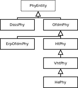
PhyEntity hierarchy
Such an architecture enables to handle the following operations in an amendment- specific manner:
WifiModehandling and data/PHY rate computation,- PPDU field size and duration computation, and
- Transmit and receive paths.
WifiPpdu
In the same vein as PhyEntity, the ns3::WifiPpdu base class has been
specialized into the following amendment-specific PPDUs:
ns3::DsssPpdu: PPDU for DSSS and HR/DSSS (11b)ns3::OfdmPpdu: PPDU for OFDM (11a and 11p)ns3::ErpOfdmPpdu: PPDU for ERP-OFDM (11g)ns3::HtPpdu: PPDU for HT (11n)ns3::VhtPpdu: PPDU for VHT (11ac)ns3::HePpdu: PPDU for HE (11ax)
Their inheritance diagram is given in Figure WifiPpdu hierarchy and closely follows the standard’s logic, e.g. section 21.3.8.1 of IEEE 802.11-2016:
:: To maintain compatibility with non-VHT STAs, specific non-VHT fields are defined that can be received by non-VHT STAs compliant with Clause 17 [OFDM] or Clause 19 [HT].
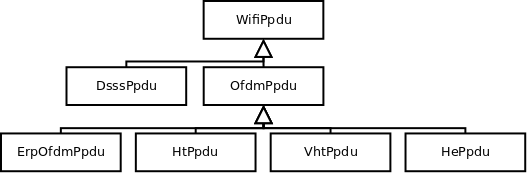
WifiPpdu hierarchy
YansWifiPhy and WifiPhyStateHelper
Class ns3::YansWifiPhy is responsible for taking packets passed to
it from the MAC (the ns3::FrameExchangeManager object) and sending them onto the
ns3::YansWifiChannel to which it is attached. It is also responsible
to receive packets from that channel, and, if reception is deemed to have
been successful, to pass them up to the MAC.
The energy of the signal intended to be received is calculated from the transmission power and adjusted based on the Tx gain of the transmitter, Rx gain of the receiver, and any path loss propagation model in effect.
Class ns3::WifiPhyStateHelper manages the state machine of the PHY
layer, and allows other objects to hook as listeners to monitor PHY
state. The main use of listeners is for the MAC layer to know when
the PHY is busy or not (for transmission and collision avoidance).
The PHY layer can be in one of seven states:
- TX: the PHY is currently transmitting a signal on behalf of its associated MAC
- RX: the PHY is synchronized on a signal and is waiting until it has received its last bit to forward it to the MAC.
- IDLE: the PHY is not in the TX, RX, or CCA_BUSY states.
- CCA_BUSY: the PHY is not in TX or RX state but the measured energy is higher than the energy detection threshold.
- SWITCHING: the PHY is switching channels.
- SLEEP: the PHY is in a power save mode and cannot send nor receive frames.
- OFF: the PHY is powered off and cannot send nor receive frames.
Packet reception works as follows. For YansWifiPhy, most of the logic
is implemented in the WifiPhy base class. The YansWifiChannel calls
WifiPhy::StartReceivePreamble (). The latter calls
PhyEntity::StartReceivePreamble () of the appropriate PHY entity
to start packet reception, but first
there is a check of the packet’s notional signal power level against a
threshold value stored in the attribute WifiPhy::RxSensitivity. Any
packet with a power lower than RxSensitivity will be dropped with no
further processing. The default value is -101 dBm, which is the thermal
noise floor for 20 MHz signal at room temperature. The purpose of this
attribute is two-fold: 1) very weak signals that will not affect the
outcome will otherwise consume simulation memory and event processing, so
they are discarded, and 2) this value can be adjusted upwards to function as
a basic carrier sense threshold limitation for experiments involving
spatial reuse considerations. Users are cautioned about the behavior of
raising this threshold; namely, that all packets with power below this
threshold will be discarded upon reception.
In StartReceivePreamble (), the packet is immediately added
to the interference helper for signal-to-noise
tracking, and then further reception steps are decided upon the state of
the PHY. In the case that the PHY is transmitting, for instance, the
packet will be dropped. If the PHY is IDLE, or if the PHY is receiving and
an optional FrameCaptureModel is being used (and the packet is within
the capture window), then PhyEntity::StartPreambleDetectionPeriod () is called next.
The PhyEntity::StartPreambleDetectionPeriod () will typically schedule an event,
PhyEntity::EndPreambleDetectionPeriod (), to occur at
the notional end of the first OFDM symbol, to check whether the preamble
has been detected. As of revisions to the model in ns-3.30, any state
machine transitions from IDLE state are suppressed until after the preamble
detection event.
The PhyEntity::EndPreambleDetectionPeriod () method will check, with a preamble detection
model, whether the signal is strong enough to be received, and if so,
an event PhyEntity::EndReceiveField () is scheduled for the end of the
preamble and the PHY is put into the CCA_BUSY state. Currently, there is only a
simple threshold-based preamble detection model in ns-3,
called ThresholdPreambleDetectionModel. If there is no preamble detection
model, the preamble is assumed to have been detected.
It is important to note that, starting with the ns-3.30 release, the default
in the WifiPhyHelper is to add the ThresholdPreambleDetectionModel with
a threshold RSSI of -82 dBm, and a threshold SNR of 4 dB. Both the RSSI
and SNR must be above these respective values for the preamble to be
successfully detected. The default sensitivity has been reduced in ns-3.30
compared with that of previous releases, so some packet receptions that were
previously successful will now fail on this check. More details on the
modeling behind this change are provided in [lanante2019].
The PhyEntity::EndReceiveField () method will check the correct reception
of the current preamble and header field and, if so, calls PhyEntity::StartReceiveField ()
for the next field,
otherwise the reception is aborted and PHY is put either in IDLE state or in CCA_BUSY state,
depending on whether the measured energy is higher than the energy detection threshold.
The next event at PhyEntity::StartReceiveField () checks, using the interference
helper and error model, whether the header was successfully decoded, and if so,
a PhyRxPayloadBegin callback (equivalent to the PHY-RXSTART primitive)
is triggered. The PHY header is often transmitted
at a lower modulation rate than is the payload. The portion of the packet
corresponding to the PHY header is evaluated for probability of error
based on the observed SNR. The InterferenceHelper object returns a value
for “probability of error (PER)” for this header based on the SNR that has
been tracked by the InterferenceHelper. The PhyEntity then draws
a random number from a uniform distribution and compares it against the
PER and decides success or failure.
This is iteratively performed up to the beginning of the data field
upon which PhyEntity::StartReceivePayload () is called.
Even if packet objects received by the PHY are not part of the reception
process, they are tracked by the InterferenceHelper object for purposes
of SINR computation and making clear channel assessment decisions.
If, in the course of reception, a packet is errored or dropped due to
the PHY being in a state in which it cannot receive a packet, the packet
is added to the interference helper, and the aggregate of the energy of
all such signals is compared against an energy detection threshold to
determine whether the PHY should enter a CCA_BUSY state.
The WifiPhy::CcaEdThreshold attribute
corresponds to what the standard calls the “ED threshold” for CCA Mode 1.
In section 16.4.8.5 in the 802.11-2012 standard: “CCA Mode 1: Energy above
threshold. CCA shall report a busy medium upon detection of any energy above
the ED threshold.” By default, this value is set to the -62 dBm level specified
in the standard for 20 MHz channels. When using YansWifiPhy, there are no
non-Wi-Fi signals, so it is unlikely that this attribute would play much of a
role in Yans wifi models if left at the default value, but if there is a strong
Wi-Fi signal that is not otherwise being received by the model, it has
the possibility to raise the CCA_BUSY while the overall energy exceeds
this threshold.
The above describes the case in which the packet is a single MPDU. For
more recent Wi-Fi standards using MPDU aggregation, StartReceivePayload
schedules an event for reception of each individual MPDU (ScheduleEndOfMpdus),
which then forwards each MPDU as they arrive up to FrameExchangeManager, if the
reception of the MPDU has been successful. Once the A-MPDU reception is finished,
FrameExchangeManager is also notified about the amount of successfully received MPDUs.
InterferenceHelper
The InterferenceHelper is an object that tracks all incoming packets and calculates probability of error values for packets being received, and also evaluates whether energy on the channel rises above the CCA threshold.
The basic operation of probability of error calculations is shown in Figure
SNIR function over time. Packets are represented as bits (not symbols) in the ns-3
model, and the InterferenceHelper breaks the packet into one or more
“chunks”, each with a different signal to noise (and interference) ratio
(SNIR). Each chunk is separately evaluated by asking for the probability
of error for a given number of bits from the error model in use. The
InterferenceHelper builds an aggregate “probability of error” value
based on these chunks and their duration, and returns this back to
the WifiPhy for a reception decision.
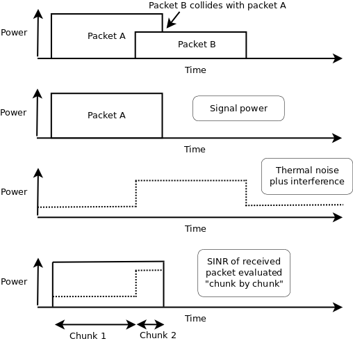
SNIR function over time
From the SNIR function we can derive the Bit Error Rate (BER) and Packet Error Rate (PER) for the modulation and coding scheme being used for the transmission.
If MIMO is used and the number of spatial streams is lower than the number of active antennas at the receiver, then a gain is applied to the calculated SNIR as follows (since STBC is not used):
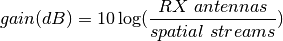
Having more TX antennas can be safely ignored for AWGN. The resulting gain is:
antennas NSS gain
2 x 1 1 0 dB
1 x 2 1 3 dB
2 x 2 1 3 dB
3 x 3 1 4.8 dB
3 x 3 2 1.8 dB
3 x 3 3 0 dB
4 x 4 1 6 dB
4 x 4 2 3 dB
4 x 4 3 1.2 dB
4 x 4 4 0 dB
...
ErrorRateModel
ns-3 makes a packet error or success decision based on the input received
SNR of a frame and based on any possible interfering frames that may overlap
in time; i.e. based on the signal-to-noise (plus interference) ratio, or
SINR. The relationship between packet error ratio (PER) and SINR in ns-3
is defined by the ns3::ErrorRateModel, of which there are several.
The PER is a function of the frame’s modulation and coding (MCS), its SINR,
and the specific ErrorRateModel configured for the MCS.
ns-3 has updated its default ErrorRateModel over time. The current
(as of ns-3.33 release) model for recent OFDM-based standards (i.e.,
802.11n/ac/ax), is the ns3::TableBasedErrorRateModel. The default
for 802.11a/g is the ns3::YansErrorRateModel, and the default for
802.11b is the ns3::DsssErrorRateModel. The error rate model for
recent standards was updated during the ns-3.33 release cycle (previously,
it was the ns3::NistErrorRateModel).
The error models are described in more detail in outside references. The current OFDM model is based on work published in [patidar2017], using link simulations results from the MATLAB WLAN Toolbox, and validated against IEEE TGn results [erceg2004]. For publications related to other error models, please refer to [pei80211ofdm], [pei80211b], [lacage2006yans], [Haccoun], [hepner2015] and [Frenger] for a detailed description of the legacy PER models.
The current ns-3 error rate models are for additive white gaussian noise channels (AWGN) only; any potential frequency-selective fading effects are not modeled.
In summary, there are four error models:
ns3::TableBasedErrorRateModel: for OFDM modes and reusesns3::DsssErrorRateModelfor 802.11b modes. This is the default for 802.11n/ac/ax.ns3::YansErrorRateModel: for OFDM modes and reusesns3::DsssErrorRateModelfor 802.11b modes. This is the default for 802.11a/g.ns3::DsssErrorRateModel: contains models for 802.11b modes. The 802.11b 1 Mbps and 2 Mbps error models are based on classical modulation analysis. If GNU Scientific Library (GSL) is installed, the 5.5 Mbps and 11 Mbps from [pursley2009] are used for CCK modulation; otherwise, results from a backup MATLAB-based CCK model are used.ns3::NistErrorRateModel: for OFDM modes and reusesns3::DsssErrorRateModelfor 802.11b modes.
Users may select either NIST, YANS or Table-based models for OFDM, and DSSS will be used in either case for 802.11b. The NIST model was a long-standing default in ns-3 (through release 3.32).
TableBasedErrorRateModel
The ns3::TableBasedErrorRateModel has been recently added and is now the ns-3 default
for 802.11n/ac/ax, while ns3::YansErrorRateModel is the ns-3 default for 802.11a/g.
Unlike analytical error models based on error bounds, ns3::TableBasedErrorRateModel contains
end-to-end link simulation tables (PER vs SNR) for AWGN channels. Since it is infeasible to generate
such look-up tables for all desired packet sizes and input SNRs, we adopt the recommendation of IEEE P802.11 TGax [porat2016] that proposed
estimating PER for any desired packet length using BCC FEC encoding by extrapolating the results from two reference lengths:
32 (all lengths less than 400) bytes and 1458 (all lengths greater or equal to 400) bytes respectively.
In case of LDPC FEC encoding, IEEE P802.11 TGax recommends the use of a single reference length.
Hence, we provide two tables for BCC and one table for LDPC that are generated using a reliable and publicly
available commercial link simulator (MATLAB WLAN Toolbox) for each modulation and coding scheme.
Note that BCC tables are limited to MCS 9. For higher MCSs, the models fall back to the use of the YANS analytical model.
The validation scenario is set as follows:
- Ideal channel and perfect channel estimation.
- Perfect packet synchronization and detection.
- Phase tracking, phase correction, phase noise, carrier frequency offset, power amplifier non-linearities etc. are not considered.
Several packets are simulated across the link to obtain PER, the number of packets needed to reliably estimate a PER value is computed using the consideration that the ratio of the estimation error to the true value should be within 10 % with probability 0.95. For each SNR value, simulations were run until a total of 40000 packets were simulated.
The obtained results are very close to TGax curves as shown in Figure Comparison of table-based OFDM Error Model with TGax results.
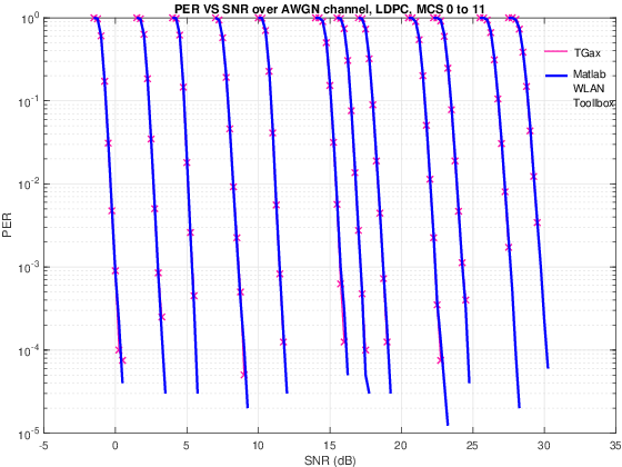
Comparison of table-based OFDM Error Model with TGax results.
Legacy ErrorRateModels
The original error rate model was called the ns3::YansErrorRateModel and
was based on analytical results. For 802.11b modulations, the 1 Mbps mode
is based on DBPSK. BER is from equation 5.2-69 from [proakis2001].
The 2 Mbps model is based on DQPSK. Equation 8 of [ferrari2004].
More details are provided in [lacage2006yans].
The ns3::NistErrorRateModel was later added.
The model was largely aligned with the previous ns3::YansErrorRateModel
for DSSS modulations 1 Mbps and 2 Mbps, but the 5.5 Mbps and 11 Mbps models
were re-based on equations (17) and (18) from [pursley2009].
For OFDM modulations, newer results were
obtained based on work previously done at NIST [miller2003]. The results
were also compared against the CMU wireless network emulator, and details
of the validation are provided in [pei80211ofdm]. Since OFDM modes use
hard-decision of punctured codes, the coded BER is calculated using
Chernoff bounds [hepner2015].
The 802.11b model was split from the OFDM model when the NIST error rate model was added, into a new model called DsssErrorRateModel.
Furthermore, the 5.5 Mbps and 11 Mbps models for 802.11b rely on library methods implemented in the GNU Scientific Library (GSL). The Waf build system tries to detect whether the host platform has GSL installed; if so, it compiles in the newer models from [pursley2009] for 5.5 Mbps and 11 Mbps; if not, it uses a backup model derived from MATLAB simulations.
The error curves for analytical models are shown to diverge from link simulation results for higher MCS in Figure YANS and NIST error model comparison with TGn results. This prompted the move to a new error model based on link simulations (the default TableBasedErrorRateModel, which provides curves close to those depicted by the TGn dashed line).
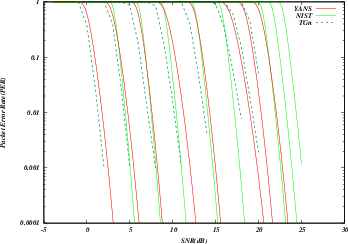
YANS and NIST error model comparison with TGn results
SpectrumWifiPhy
This section describes the implementation of the SpectrumWifiPhy
class that can be found in src/wifi/model/spectrum-wifi-phy.{cc,h}.
The implementation also makes use of additional classes found in the same directory:
wifi-spectrum-phy-interface.{cc,h}wifi-spectrum-signal-parameters.{cc,h}
and classes found in the spectrum module:
wifi-spectrum-value-helper.{cc,h}
The current SpectrumWifiPhy class
reuses the existing interference manager and error rate models originally
built for YansWifiPhy, but allows, as a first step, foreign (non Wi-Fi)
signals to be treated as additive noise.
Two main changes were needed to adapt the Spectrum framework to Wi-Fi.
First, the physical layer must send signals compatible with the
Spectrum channel framework, and in particular, the
MultiModelSpectrumChannel that allows signals from different
technologies to coexist. Second, the InterferenceHelper must be
extended to support the insertion of non-Wi-Fi signals and to
add their received power to the noise, in the same way that
unintended Wi-Fi signals (perhaps from a different SSID or arriving
late from a hidden node) are added to the noise.
Unlike YansWifiPhy, where there are no foreign signals, CCA_BUSY state
will be raised for foreign signals that are higher than CcaEdThreshold
(see section 16.4.8.5 in the 802.11-2012 standard for definition of
CCA Mode 1). The attribute WifiPhy::CcaEdThreshold therefore
potentially plays a larger role in this model than in the YansWifiPhy
model.
To support the Spectrum channel, the YansWifiPhy transmit and receive methods
were adapted to use the Spectrum channel API. This required developing
a few SpectrumModel-related classes. The class
WifiSpectrumValueHelper is used to create Wi-Fi signals with the
spectrum framework and spread their energy across the bands. The
spectrum is sub-divided into sub-bands (the width of an OFDM
subcarrier, which depends on the technology). The power allocated to a particular channel
is spread across the sub-bands roughly according to how power would
be allocated to sub-carriers. Adjacent channels are models by the use of
OFDM transmit spectrum masks as defined in the standards.
To support an easier user configuration experience, the existing
YansWifi helper classes (in src/wifi/helper) were copied and
adapted to provide equivalent SpectrumWifi helper classes.
Finally, for reasons related to avoiding C++ multiple inheritance
issues, a small forwarding class called WifiSpectrumPhyInterface
was inserted as a shim between the SpectrumWifiPhy and the
Spectrum channel. The WifiSpectrumPhyInterface calls a different
SpectrumWifiPhy::StartRx () method to start the reception process.
This method performs the check of the signal power against the
WifiPhy::RxSensitivity attribute and discards weak signals, and
also checks if the signal is a Wi-Fi signal; non-Wi-Fi signals are added
to the InterferenceHelper and can raise CCA_BUSY but are not further processed
in the reception chain. After this point, valid Wi-Fi signals cause
WifiPhy::StartReceivePreamble to be called, and the processing continues
as described above.
The MAC model
Infrastructure association
Association in infrastructure mode is a high-level MAC function. Either active probing or passive scanning is used (default is passive scan). At the start of the simulation, Wi-Fi network devices configured as STA will attempt to scan the channel. Depends on whether passive or active scanning is selected, STA will attempt to gather beacons, or send a probe request and gather probe responses until the respective timeout occurs. The end result will be a list of candidate AP to associate to. STA will then try to associate to the best AP (i.e., best SNR).
If association is rejected by the AP for some reason, the STA will try to associate to the next best AP until the candidate list is exhausted which then sends STA to ‘REFUSED’ state. If this occurs, the simulation user will need to force reassociation retry in some way, perhaps by changing configuration (i.e. the STA will not persistently try to associate upon a refusal).
When associated, if the configuration is changed by the simulation user, the STA will try to reassociate with the existing AP.
If the number of missed beacons exceeds the threshold, the STA will notify the rest of the device that the link is down (association is lost) and restart the scanning process. Note that this can also happen when an association request fails without explicit refusal (i.e., the AP fails to respond to association request).
Roaming
Roaming at layer-2 (i.e. a STA migrates its association from one AP to another) is not presently supported. Because of that, the Min/Max channel dwelling time implementation as described by the IEEE 802.11 standard [ieee80211] is also omitted, since it is only meaningful on the context of channel roaming.
Channel access
The 802.11 Distributed Coordination Function is used to calculate when to grant access to the transmission medium. While implementing the DCF would have been particularly easy if we had used a recurring timer that expired every slot, we chose to use the method described in [ji2004sslswn] where the backoff timer duration is lazily calculated whenever needed since it is claimed to have much better performance than the simpler recurring timer solution.
The DCF basic access is described in section 10.3.4.2 of [ieee80211-2016].
- “A STA may transmit an MPDU when it is operating under the DCF access method [..] when the STA determines that the medium is idle when a frame is queued for transmission, and remains idle for a period of a DIFS, or an EIFS (10.3.2.3.7) from the end of the immediately preceding medium-busy event, whichever is the greater, and the backoff timer is zero. Otherwise the random backoff procedure described in 10.3.4.3 shall be followed.”
Thus, a station is allowed not to invoke the backoff procedure if all of the following conditions are met:
- the medium is idle when a frame is queued for transmission
- the medium remains idle until the most recent of these two events: a DIFS from the time when the frame is queued for transmission; an EIFS from the end of the immediately preceding medium-busy event (associated with the reception of an erroneous frame)
- the backoff timer is zero
The backoff procedure of DCF is described in section 10.3.4.3 of [ieee80211-2016].
- “A STA shall invoke the backoff procedure to transfer a frame when finding the medium busy as indicated by either the physical or virtual CS mechanism.”
- “A backoff procedure shall be performed immediately after the end of every transmission with the More Fragments bit set to 0 of an MPDU of type Data, Management, or Control with subtype PS-Poll, even if no additional transmissions are currently queued.”
The EDCA backoff procedure is slightly different than the DCF backoff procedure and is described in section 10.22.2.2 of [ieee80211-2016]. The backoff procedure shall be invoked by an EDCAF when any of the following events occur:
- a frame is “queued for transmission such that one of the transmit queues associated with that AC has now become non-empty and any other transmit queues associated with that AC are empty; the medium is busy on the primary channel”
- “The transmission of the MPDU in the final PPDU transmitted by the TXOP holder during the TXOP for that AC has completed and the TXNAV timer has expired, and the AC was a primary AC”
- “The transmission of an MPDU in the initial PPDU of a TXOP fails [..] and the AC was a primary AC”
- “The transmission attempt collides internally with another EDCAF of an AC that has higher priority”
- (optionally) “The transmission by the TXOP holder of an MPDU in a non-initial PPDU of a TXOP fails”
Additionally, section 10.22.2.4 of [ieee80211-2016] introduces the notion of slot boundary, which basically occurs following SIFS + AIFSN * slotTime of idle medium after the last busy medium that was the result of a reception of a frame with a correct FCS or following EIFS - DIFS + AIFSN * slotTime + SIFS of idle medium after the last indicated busy medium that was the result of a frame reception that has resulted in FCS error, or following a slotTime of idle medium occurring immediately after any of these conditions.
On these specific slot boundaries, each EDCAF shall make a determination to perform one and only one of the following functions:
- Decrement the backoff timer.
- Initiate the transmission of a frame exchange sequence.
- Invoke the backoff procedure due to an internal collision.
- Do nothing.
Thus, if an EDCAF decrements its backoff timer on a given slot boundary and, as a result, the backoff timer has a zero value, the EDCAF cannot immediately transmit, but it has to wait for another slotTime of idle medium before transmission can start.
The higher-level MAC functions are implemented in a set of other C++ classes and deal with:
- packet fragmentation and defragmentation,
- use of the RTS/CTS protocol,
- rate control algorithm,
- connection and disconnection to and from an Access Point,
- the MAC transmission queue,
- beacon generation,
- MSDU aggregation,
- etc.
Frame Exchange Managers
As the IEEE 802.11 standard evolves, more and more features are added and it is more and more difficult to have a single component handling all of the allowed frame exchange sequences. A hierarchy of FrameExchangeManager classes has been introduced to make the code clean and scalable, while avoiding code duplication. Each FrameExchangeManager class handles the frame exchange sequences introduced by a given amendment. The FrameExchangeManager hierarchy is depicted in Figure FrameExchangeManager hierarchy.
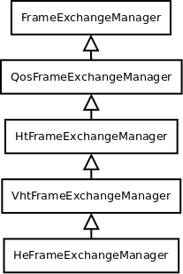
FrameExchangeManager hierarchy
The features supported by every FrameExchangeManager class are as follows:
FrameExchangeManageris the base class. It handles the basic sequences for non-QoS stations: MPDU followed by Normal Ack, RTS/CTS and CTS-to-self, NAV setting and resetting, MPDU fragmentationQosFrameExchangeManageradds TXOP support: multiple protection setting, TXOP truncation via CF-End, TXOP recovery, ignore NAV when responding to an RTS sent by the TXOP holderHtFrameExchangeManageradds support for Block Ack (compressed variant), A-MSDU and A-MPDU aggregation, Implicit Block Ack Request policyVhtFrameExchangeManageradds support for S-MPDUsHeFrameExchangeManageradds support for the transmission and reception of multi-user frames via DL OFDMA and UL OFDMA, as detailed below.
Multi-user transmissions
Since the introduction of the IEEE 802.11ax amendment, multi-user (MU) transmissions are possible, both in downlink (DL) and uplink (UL), by using OFDMA and/or MU-MIMO. Currently, ns-3 only supports multi-user transmissions via OFDMA. Three acknowledgment sequences are implemented for DL OFDMA.
The first acknowledgment sequence is made of multiple BlockAckRequest/BlockAck frames sent as single-user frames, as shown in Figure Acknowledgment of DL MU frames in single-user format.
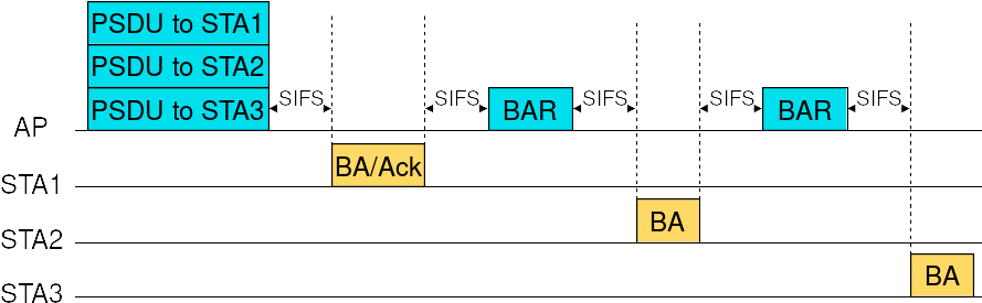
Acknowledgment of DL MU frames in single-user format
For the second acknowledgment sequence, an MU-BAR Trigger Frame is sent (as a single-user frame) to solicit BlockAck responses sent in TB PPDUs, as shown in Figure Acknowledgment of DL MU frames via MU-BAR Trigger Frame sent as single-user frame.
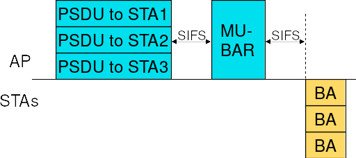
Acknowledgment of DL MU frames via MU-BAR Trigger Frame sent as single-user frame
For the third acknowledgment sequence, an MU-BAR Trigger Frame is aggregated to every PSDU included in the DL MU PPDU and the BlockAck responses are sent in TB PPDUs, as shown in Figure Acknowledgment of DL MU frames via aggregated MU-BAR Trigger Frames.
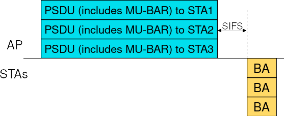
Acknowledgment of DL MU frames via aggregated MU-BAR Trigger Frames
For UL OFDMA, both BSRP Trigger Frames and Basic Trigger Frames are supported, as shown in Figure Acknowledgment of DL MU frames via aggregated MU-BAR Trigger Frames. A BSRP Trigger Frame is sent by an AP to solicit stations to send QoS Null frames containing Buffer Status Reports. A Basic Trigger Frame is sent by an AP to solicit stations to send data frames in TB PPDUs, which are acknowledged by the AP via a Multi-STA BlockAck frame.
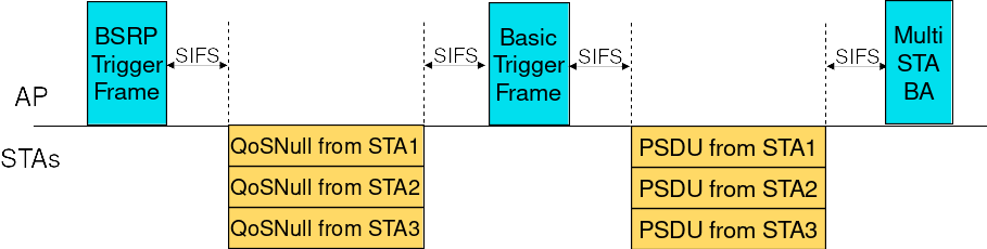
Acknowledgment of DL MU frames via aggregated MU-BAR Trigger Frames
Multi-User Scheduler
A new component, named MultiUserScheduler, is in charge of determining what frame exchange
sequence the aggregated AP has to perform when gaining a TXOP (DL OFDMA, UL OFDMA or BSRP Trigger
Frame), along with the information needed to perform the selected frame exchange sequence (e.g.,
the set of PSDUs to send in case of DL OFDMA). MultiUserScheduler is an abstract base class.
Currently, the only available subclass is RrMultiUserScheduler. By default, no multi-user
scheduler is aggregated to an AP (hence, OFDMA is not enabled).
Round-robin Multi-User Scheduler
The Round-robin Multi-User Scheduler dynamically assigns a priority to each station to ensure
airtime fairness in the selection of stations for DL multi-user transmissions. The NStations
attribute enables to set the maximum number of stations that can be the recipients of a DL
multi-user frame. Therefore, every time an HE AP accesses the channel to transmit a DL
multi-user frame, the scheduler determines the number of stations the AP has frames to send
to (capped at the value specified through the mentioned attribute) and attempts to allocate
equal sized RUs to as many such stations as possible without leaving RUs of the same size
unused. For instance, if the channel bandwidth is 40 MHz and the determined number of stations
is 5, the first 4 stations (in order of priority) are allocated a 106-tone RU each (if 52-tone
RUs were allocated, we would have three 52-tone RUs unused). If central 26-tone RUs can be
allocated (as determined by the UseCentral26TonesRus attribute), possible stations that
have not been allocated an RU are assigned one of such 26-tone RU. In the previous example,
the fifth station would have been allocated one of the two available central 26-tone RUs.
When UL OFDMA is enabled (via the EnableUlOfdma attribute), every DL OFDMA frame exchange
is followed by an UL OFDMA frame exchange involving the same set of stations and the same RU
allocation as the preceding DL multi-user frame. The transmission of a BSRP Trigger Frame can
optionally (depending on the value of the EnableBsrp attribute) precede the transmission
of a Basic Trigger Frame in order for the AP to collect information about the buffer status
of the stations.
Ack manager
Since the introduction of the IEEE 802.11e amendment, multiple acknowledgment policies are available, which are coded in the Ack Policy subfield in the QoS Control field of QoS Data frames (see Section 9.2.4.5.4 of the IEEE 802.11-2016 standard). For instance, an A-MPDU can be sent with the Normal Ack or Implicit Block Ack Request policy, in which case the receiver replies with a Normal Ack or a Block Ack depending on whether the A-MPDU contains a single MPDU or multiple MPDUs, or with the Block Ack policy, in which case the receiver waits to receive a Block Ack Request in the future to which it replies with a Block Ack.
WifiAckManager is the abstract base class introduced to provide an interface
for multiple ack managers. Currently, the default ack manager is
the WifiDefaultAckManager.
WifiDefaultAckManager
The WifiDefaultAckManager allows to determine which acknowledgment policy
to use depending on the value of its attributes:
UseExplicitBar: used to determine the ack policy to use when a response is needed from the recipient and the current transmission includes multiple frames (A-MPDU) or there are frames transmitted previously for which an acknowledgment is needed. If this attribute is true, the Block Ack policy is used. Otherwise, the Implicit Block Ack Request policy is used.BaThreshold: used to determine when the originator of a Block Ack agreement needs to request a response from the recipient. A value of zero means that a response is requested at every frame transmission. Otherwise, a non-zero value (less than or equal to 1) means that a response is requested upon transmission of a frame whose sequence number is distant at least BaThreshold multiplied by the transmit window size from the starting sequence number of the transmit window.DlMuAckSequenceType: used to select the acknowledgment sequence for DL MU frames (acknowledgment in single-user format, acknowledgment via MU-BAR Trigger Frame sent as single-user frame, or acknowledgment via MU-BAR Trigger Frames aggregated to the data frames).
Protection manager
The protection manager is in charge of determining the protection mechanism to use, if any, when sending a frame.
WifiProtectionManager is the abstract base class introduced to provide an interface
for multiple protection managers. Currently, the default protection manager is
the WifiDefaultProtectionManager.
WifiDefaultProtectionManager
The WifiDefaultProtectionManager selects a protection mechanism based on the
information provided by the remote station manager.
Rate control algorithms
Multiple rate control algorithms are available in ns-3. Some rate control algorithms are modeled after real algorithms used in real devices; others are found in literature. The following rate control algorithms can be used by the MAC low layer:
Algorithms found in real devices:
ArfWifiManager(default forWifiHelper)OnoeWifiManagerConstantRateWifiManagerMinstrelWifiManagerMinstrelHtWifiManager
Algorithms in literature:
IdealWifiManagerAarfWifiManager[lacage2004aarfamrr]AmrrWifiManager[lacage2004aarfamrr]CaraWifiManager[kim2006cara]RraaWifiManager[wong2006rraa]AarfcdWifiManager[maguolo2008aarfcd]ParfWifiManager[akella2007parf]AparfWifiManager[chevillat2005aparf]ThompsonSamplingWifiManager[krotov2020rate]
ConstantRateWifiManager
The constant rate control algorithm always uses the same transmission mode for every packet. Users can set a desired ‘DataMode’ for all ‘unicast’ packets and ‘ControlMode’ for all ‘request’ control packets (e.g. RTS).
To specify different data mode for non-unicast packets, users must set the ‘NonUnicastMode’ attribute of the WifiRemoteStationManager. Otherwise, WifiRemoteStationManager will use a mode with the lowest rate for non-unicast packets.
The 802.11 standard is quite clear on the rules for selection of transmission parameters for control response frames (e.g. CTS and ACK). ns-3 follows the standard and selects the rate of control response frames from the set of basic rates or mandatory rates. This means that control response frames may be sent using different rate even though the ConstantRateWifiManager is used. The ControlMode attribute of the ConstantRateWifiManager is used for RTS frames only. The rate of CTS and ACK frames are selected according to the 802.11 standard. However, users can still manually add WifiMode to the basic rate set that will allow control response frames to be sent at other rates. Please consult the project wiki on how to do this.
Available attributes:
- DataMode (default WifiMode::OfdmRate6Mbps): specify a mode for all non-unicast packets
- ControlMode (default WifiMode::OfdmRate6Mbps): specify a mode for all ‘request’ control packets
IdealWifiManager
The ideal rate control algorithm selects the best
mode according to the SNR of the previous packet sent.
Consider node A sending a unicast packet to node B.
When B successfully receives the packet sent from A,
B records the SNR of the received packet into a ns3::SnrTag
and adds the tag to an ACK back to A.
By doing this, A is able to learn the SNR of the packet sent to B
using an out-of-band mechanism (thus the name ‘ideal’).
A then uses the SNR to select a transmission mode based
on a set of SNR thresholds, which was built from a target BER and
mode-specific SNR/BER curves.
Available attribute:
- BerThreshold (default 1e-6): The maximum Bit Error Rate that is used to calculate the SNR threshold for each mode.
Note that the BerThreshold has to be low enough to select a robust enough MCS (or mode) for a given SNR value, without being too restrictive on the target BER. Indeed we had noticed that the previous default value (i.e. 1e-5) led to the selection of HE MCS-11 which resulted in high PER. With this new default value (i.e. 1e-6), a HE STA moving away from a HE AP has smooth throughput decrease (whereas with 1e-5, better performance was seen further away, which is not “ideal”).
ThompsonSamplingWifiManager
Thompson Sampling (TS) is a classical solution to the Multi-Armed Bandit problem. ThompsonSamplingWifiManager implements a rate control algorithm based on TS with the goal of providing a simple statistics-based algorithm with a low number of parameters.
The algorithm maintains the number of successful transmissions
 and the number of unsuccessful transmissions
 for each MCS , both of which are initially
set to zero.
for each MCS , both of which are initially
set to zero.
To select MCS for a data frame, the algorithm draws a sample frame
success rate  from the beta distribution with shape
parameters
from the beta distribution with shape
parameters  for each MCS and then
selects MCS with the highest expected throughput calculated as the
sample frame success rate multiplied by MCS rate.
for each MCS and then
selects MCS with the highest expected throughput calculated as the
sample frame success rate multiplied by MCS rate.
To account for changing channel conditions, exponential decay is
applied to and . The rate of
exponential decay is controlled with the Decay attribute which is
the inverse of the time constant. Default value of 1 Hz results in
using exponential window with the time constant of 1 second. Setting
this value to zero effectively disables exponential decay and can be
used in static scenarios.
Control frames are always transmitted using the most robust MCS, except when the standard specifies otherwise, such as for ACK frames.
As the main goal of this algorithm is to provide a stable baseline, it does not take into account backoff overhead, inter-frame spaces and aggregation for MCS rate calculation. For an example of a more complex statistics-based rate control algorithm used in real devices, consider Minstrel-HT described below.
MinstrelWifiManager
The minstrel rate control algorithm is a rate control algorithm originated from madwifi project. It is currently the default rate control algorithm of the Linux kernel.
Minstrel keeps track of the probability of successfully sending a frame of each available rate. Minstrel then calculates the expected throughput by multiplying the probability with the rate. This approach is chosen to make sure that lower rates are not selected in favor of the higher rates (since lower rates are more likely to have higher probability).
In minstrel, roughly 10 percent of transmissions are sent at the so-called lookaround rate. The goal of the lookaround rate is to force minstrel to try higher rate than the currently used rate.
For a more detailed information about minstrel, see [linuxminstrel].
MinstrelHtWifiManager
This is the extension of minstrel for 802.11n/ac/ax.
802.11ax OBSS PD spatial reuse
802.11ax mode supports OBSS PD spatial reuse feature. OBSS PD stands for Overlapping Basic Service Set Preamble-Detection. OBSS PD is an 802.11ax specific feature that allows a STA, under specific conditions, to ignore an inter-BSS PPDU.
OBSS PD Algorithm
ObssPdAlgorithm is the base class of OBSS PD algorithms.
It implements the common functionalities. First, it makes sure the necessary callbacks are setup.
Second, when a PHY reset is requested by the algorithm, it performs the computation to determine the TX power
restrictions and informs the PHY object.
The PHY keeps tracks of incoming requests from the MAC to get access to the channel. If a request is received and if PHY reset(s) indicating TX power limitations occured before a packet was transmitted, the next packet to be transmitted will be sent with a reduced power. Otherwise, no TX power restrictions will be applied.
Constant OBSS PD Algorithm
Constant OBSS PD algorithm is a simple OBSS PD algorithm implemented in the ConstantObssPdAlgorithm class.
Once a HE preamble and its header have been received by the PHY, ConstantObssPdAlgorithm::
ReceiveHeSig is triggered.
The algorithm then checks whether this is an OBSS frame by comparing its own BSS color with the BSS color of the received preamble.
If this is an OBSS frame, it compares the received RSSI with its configured OBSS PD level value. The PHY then gets reset to IDLE
state in case the received RSSI is lower than that constant OBSS PD level value, and is informed about a TX power restrictions.
Note: since our model is based on a single threshold, the PHY only supports one restricted power level.
Modifying Wifi model
Modifying the default wifi model is one of the common tasks when performing research. We provide an overview of how to make changes to the default wifi model in this section. Depending on your goal, the common tasks are (in no particular order):
- Creating or modifying the default Wi-Fi frames/headers by making changes to
wifi-mac-header.*. - MAC low modification. For example, handling new/modified control frames (think RTS/CTS/ACK/Block ACK),
making changes to two-way transaction/four-way transaction. Users usually make changes to
frame-exchange-manager.*or its subclasses to accomplish this. Handling of control frames is performed inFrameExchangeManager::ReceiveMpdu. - MAC high modification. For example, handling new management frames (think beacon/probe),
beacon/probe generation. Users usually make changes to
regular-wifi-mac.*,``sta-wifi-mac.*``,ap-wifi-mac.*, oradhoc-wifi-mac.*to accomplish this. - Wi-Fi queue management. The files
txop.*andqos-txop.*are of interest for this task. - Channel access management. Users should modify the files
channel-access-manager.*, which grant access toTxopandQosTxop. - Fragmentation and RTS threholds are handled by Wi-Fi remote station manager. Note that Wi-Fi remote
station manager simply indicates if fragmentation and RTS are needed. Fragmentation is handled by
TxoporQosTxopwhile RTS/CTS transaction is handled byFrameExchangeManager. - Modifying or creating new rate control algorithms can be done by creating a new child class of Wi-Fi remote station manager or modifying the existing ones.
User Documentation
Using the WifiNetDevice
The modularity provided by the implementation makes low-level configuration of the WifiNetDevice powerful but complex. For this reason, we provide some helper classes to perform common operations in a simple matter, and leverage the ns-3 attribute system to allow users to control the parameterization of the underlying models.
Users who use the low-level ns-3 API and who wish to add a WifiNetDevice to
their node must create an instance of a WifiNetDevice, plus a number of
constituent objects, and bind them together appropriately (the WifiNetDevice is
very modular in this regard, for future extensibility). At the low-level API,
this can be done with about 20 lines of code (see ns3::WifiHelper::Install,
and ns3::YansWifiPhyHelper::Create). They also must create, at some point, a
Channel, which also contains a number of constituent objects (see
ns3::YansWifiChannelHelper::Create).
However, a few helpers are available for users to add these devices and channels
with only a few lines of code, if they are willing to use defaults, and the
helpers provide additional API to allow the passing of attribute values to
change default values. Commonly used attribute values are listed in the
Attributes section. The scripts in examples/wireless can be browsed to
see how this is done. Next, we describe the common steps to create a WifiNetDevice
from the bottom layer (Channel) up to the device layer (WifiNetDevice).
To create a WifiNetDevice, users need to follow these steps:
- Decide on which physical layer framework, the
SpectrumWifiPhyorYansWifiPhy, to use. This will affect which Channel and Phy type to use. - Configure the Channel: Channel takes care of getting signal from one device to other devices on the same Wi-Fi channel. The main configurations of WifiChannel are propagation loss model and propagation delay model.
- Configure the WifiPhy: WifiPhy takes care of actually sending and receiving wireless signal from Channel. Here, WifiPhy decides whether each frame will be successfully decoded or not depending on the received signal strength and noise. Thus, the main configuration of WifiPhy is the error rate model, which is the one that actually calculates the probability of successfully decoding the frame based on the signal.
- Configure WifiMac: this step is more related to the architecture and device level. The users configure the wifi architecture (i.e. ad-hoc or ap-sta) and whether QoS (802.11e), HT (802.11n) and/or VHT (802.11ac) and/or HE (802.11ax) features are supported or not.
- Create WifiDevice: at this step, users configure the desired wifi standard (e.g. 802.11b, 802.11g, 802.11a, 802.11n, 802.11ac or 802.11ax) and rate control algorithm.
- Configure mobility: finally, a mobility model is (usually) required before WifiNetDevice can be used; even if the devices are stationary, their relative positions are needed for propagation loss calculations.
The following sample code illustrates a typical configuration using mostly default values in the simulator, and infrastructure mode:
NodeContainer wifiStaNode;
wifiStaNode.Create (10); // Create 10 station node objects
NodeContainer wifiApNode;
wifiApNode.Create (1); // Create 1 access point node object
// Create a channel helper and phy helper, and then create the channel
YansWifiChannelHelper channel = YansWifiChannelHelper::Default ();
YansWifiPhyHelper phy = YansWifiPhyHelper::Default ();
phy.SetChannel (channel.Create ());
// Create a WifiMacHelper, which is reused across STA and AP configurations
WifiMacHelper mac;
// Create a WifiHelper, which will use the above helpers to create
// and install Wifi devices. Configure a Wifi standard to use, which
// will align various parameters in the Phy and Mac to standard defaults.
WifiHelper wifi;
wifi.SetStandard (WIFI_STANDARD_80211n_5GHZ);
// Declare NetDeviceContainers to hold the container returned by the helper
NetDeviceContainer wifiStaDevices;
NetDeviceContainer wifiApDevice;
// Perform the installation
mac.SetType ("ns3::StaWifiMac");
wifiStaDevices = wifi.Install (phy, mac, wifiStaNodes);
mac.SetType ("ns3::ApWifiMac");
wifiApDevice = wifi.Install (phy, mac, wifiApNode);
At this point, the 11 nodes have Wi-Fi devices configured, attached to a common channel. The rest of this section describes how additional configuration may be performed.
YansWifiChannelHelper
The YansWifiChannelHelper has an unusual name. Readers may wonder why it is named this way. The reference is to the yans simulator from which this model is taken. The helper can be used to create a YansWifiChannel with a default PropagationLoss and PropagationDelay model.
Users will typically type code such as:
YansWifiChannelHelper wifiChannelHelper = YansWifiChannelHelper::Default ();
Ptr<Channel> wifiChannel = wifiChannelHelper.Create ();
to get the defaults. Specifically, the default is a channel model with a
propagation delay equal to a constant, the speed of light (ns3::ConstantSpeedPropagationDelayModel),
and a propagation loss based on a default log distance model (ns3::LogDistancePropagationLossModel), using a default exponent of 3.
Please note that the default log distance model is configured with a reference
loss of 46.6777 dB at reference distance of 1m. The reference loss of 46.6777 dB
was calculated using Friis propagation loss model at 5.15 GHz. The reference loss
must be changed if 802.11b, 802.11g, 802.11n (at 2.4 GHz) or 802.11ax (at 2.4 GHz) are used since they operate at 2.4 Ghz.
Note the distinction above in creating a helper object vs. an actual simulation
object. In ns-3, helper objects (used at the helper API only) are created on
the stack (they could also be created with operator new and later deleted).
However, the actual ns-3 objects typically inherit from class ns3::Object
and are assigned to a smart pointer. See the chapter in the ns-3 manual for
a discussion of the ns-3 object model, if you are not familiar with it.
The following two methods are useful when configuring YansWifiChannelHelper:
YansWifiChannelHelper::AddPropagationLossadds a PropagationLossModel; if one or more PropagationLossModels already exist, the new model is chained to the endYansWifiChannelHelper::SetPropagationDelaysets a PropagationDelayModel (not chainable)
YansWifiPhyHelper
Physical devices (base class ns3::WifiPhy) connect to ns3::YansWifiChannel models in
ns-3. We need to create WifiPhy objects appropriate for the YansWifiChannel; here
the YansWifiPhyHelper will do the work.
The YansWifiPhyHelper class configures an object factory to create instances of
a YansWifiPhy and adds some other objects to it, including possibly a
supplemental ErrorRateModel and a pointer to a MobilityModel. The user code is
typically:
YansWifiPhyHelper wifiPhyHelper;
wifiPhyHelper.SetChannel (wifiChannel);
The default YansWifiPhyHelper is configured with TableBasedErrorRateModel
(ns3::TableBasedErrorRateModel). You can change the error rate model by
calling the YansWifiPhyHelper::SetErrorRateModel method.
Optionally, if pcap tracing is needed, a user may use the following command to enable pcap tracing:
YansWifiPhyHelper::SetPcapDataLinkType (enum SupportedPcapDataLinkTypes dlt)
ns-3 supports RadioTap and Prism tracing extensions for 802.11.
Note that we haven’t actually created any WifiPhy objects yet; we’ve just prepared the YansWifiPhyHelper by telling it which channel it is connected to. The Phy objects are created in the next step.
In order to enable 802.11n/ac/ax MIMO, the number of antennas as well as the number of supported spatial streams need to be configured. For example, this code enables MIMO with 2 antennas and 2 spatial streams:
wifiPhyHelper.Set ("Antennas", UintegerValue (2));
wifiPhyHelper.Set ("MaxSupportedTxSpatialStreams", UintegerValue (2));
wifiPhyHelper.Set ("MaxSupportedRxSpatialStreams", UintegerValue (2));
It is also possible to configure less streams than the number of antennas in order to benefit from diversity gain, and to define different MIMO capabilities for downlink and uplink. For example, this code configures a node with 3 antennas that supports 2 spatial streams in downstream and 1 spatial stream in upstream:
wifiPhyHelper.Set ("Antennas", UintegerValue (3));
wifiPhyHelper.Set ("MaxSupportedTxSpatialStreams", UintegerValue (2));
wifiPhyHelper.Set ("MaxSupportedRxSpatialStreams", UintegerValue (1));
802.11n PHY layer can support both 20 (default) or 40 MHz channel width, and 802.11ac/ax PHY layer can use either 20, 40, 80 (default) or 160 MHz channel width. See below for further documentation on setting the frequency, channel width, and channel number.
WifiHelper wifi;
wifi.SetStandard (WIFI_STANDARD_80211ac);
wifi.SetRemoteStationManager ("ns3::ConstantRateWifiManager",
"DataMode", StringValue ("VhtMcs9"),
"ControlMode", StringValue ("VhtMcs0"));
//Install PHY and MAC
Ssid ssid = Ssid ("ns3-wifi");
WifiMacHelper mac;
mac.SetType ("ns3::StaWifiMac",
"Ssid", SsidValue (ssid),
"ActiveProbing", BooleanValue (false));
NetDeviceContainer staDevice;
staDevice = wifi.Install (phy, mac, wifiStaNode);
mac.SetType ("ns3::ApWifiMac",
"Ssid", SsidValue (ssid));
NetDeviceContainer apDevice;
apDevice = wifi.Install (phy, mac, wifiApNode);
Channel, frequency, and channel width configuration
There are a few ns3::WifiPhy parameters that are related, and cannot
be set completely independently, concerning the frequency and channel width
that the device is tuned to. These are:
WifiPhyStandard: For example, 802.11b, 802.11n, etc.FrequencyChannelWidthChannelNumber
It is possible to set the above to incompatible combinations (e.g. channel number 1 with 40 MHz channel width on frequency 4915 MHz). In addition, the latter three values above are attributes; it is possible to set them in a number of ways:
- by setting global configuration default; e.g.
Config::SetDefault ("ns3::WifiPhy::ChannelNumber", UintegerValue (3));
- by setting an attribute value in the helper; e.g.
YansWifiPhyHelper wifiPhyHelper = YansWifiPhyHelper::Default ();
wifiPhyHelper.Set ("ChannelNumber", UintegerValue (3));
- by setting the WifiHelper::SetStandard (enum WifiStandard) method; and
- by performing post-installation configuration of the option, either via a Ptr to the WifiPhy object, or through the Config namespace; e.g.:
Config::Set ("/NodeList/0/DeviceList/*/$ns3::WifiNetDevice/Phy/$ns3::WifiPhy/ChannelNumber",
UintegerValue (3));
This section provides guidance on how to configure these settings in a coherent manner, and what happens if non-standard values are chosen.
WifiHelper::SetStandard()
WifiHelper::SetStandard () is a method to set various parameters
in the Mac and Phy to standard values and some reasonable defaults.
For example, SetStandard (WIFI_STANDARD_80211a) will set the
WifiPhy to Channel 36 in the 5 GHz band, among other settings appropriate
for 802.11a.
The following values for WifiStandard are defined in
src/wifi/model/wifi-standards.h:
WIFI_STANDARD_80211a,
WIFI_STANDARD_80211b,
WIFI_STANDARD_80211g,
WIFI_STANDARD_80211p,
WIFI_STANDARD_80211n_2_4GHZ,
WIFI_STANDARD_80211n_5GHZ,
WIFI_STANDARD_80211ac,
WIFI_STANDARD_80211ax_2_4GHZ,
WIFI_STANDARD_80211ax_5GHZ,
WIFI_STANDARD_80211ax_6GHZ
By default, the WifiHelper (the typical use case for WifiPhy creation) will configure the WIFI_STANDARD_80211a standard by default. Other values for standards should be passed explicitly to the WifiHelper object.
If user has not already separately configured Frequency or ChannelNumber when SetStandard is called, the user obtains default values, in addition (e.g. channel 1 for 802.11b/g, or channel 36 for a/n), in addition to an appropriate ChannelWidth value for the standard (typically, 20 MHz, but 80 MHz for 802.11ac/ax).
WifiPhy attribute interactions
Users should keep in mind that the two attributes that matter most
within the model code are WifiPhy::Frequency and
WifiPhy::ChannelWidth; these are the ones directly used to set
transmission parameters. WifiPhy::ChannelNumber and
WifiHelper::SetStandard () are convenience shorthands for setting
frequency and channel width. The ns3::WifiPhy contains code to
keep these values aligned and to generate runtime errors in some cases
if users set these attributes to incompatible values.
The pair (WifiPhyStandard, ChannelNumber) is an alias for a pair of (Frequency/ChannelWidth) items. Valid combinations are stored in a map within WifiPhy that is populated with well-known values but that can be dynamically extended at runtime.
WifiPhy::Frequency
The WifiPhy channel center frequency is set by the attribute Frequency
in the class WifiPhy. It is expressed in units of MHz. By default,
this attribute is set to the value 0 to indicate that no value is configured.
Note that this is a change in definition from ns-3.25 and earlier releases, where this attribute referred to the start of the overall frequency band on which the channel resides, not the specific channel center frequency.
WifiPhy::ChannelWidth
The WifiPhy channel width is set by the attribute ChannelWidth
in the class WifiPhy. It is expressed in units of MHz. By default,
this attribute is set to the value 20. Allowable values are 5, 10, 20,
22, 40, 80, or 160 (MHz).
WifiPhy::ChannelNumber
Several channel numbers are defined and well-known in practice. However, valid channel numbers vary by geographical region around the world, and there is some overlap between the different standards.
In ns-3, the class WifiPhy contains an attribute ChannelNumber that
is, by default, set to the value 0. The value 0 indicates that no
channel number has been set by the user.
In ns-3, a ChannelNumber may be defined or unknown. These terms are not found in the code; they are just used to describe behavior herein.
If a ChannelNumber is defined, it means that WifiPhy has stored a map of ChannelNumber to the center frequency and channel width commonly known for that channel in practice. For example:
- Channel 1, when IEEE 802.11b is configured, corresponds to a channel width of 22 MHz and a center frequency of 2412 MHz.
- Channel 36, when IEEE 802.11n is configured at 5 GHz, corresponds to a channel width of 20 MHz and a center frequency of 5180 MHz.
The following channel numbers are well-defined for 2.4 GHz standards:
- channels 1-14 with ChannelWidth of 22 MHz for 802.11b
- channels 1-14 with ChannelWidth of 20 MHz for 802.11n-2.4GHz and 802.11g
The following channel numbers are well-defined for 5 GHz standards:
ChannelWidth |
ChannelNumber |
| 20 MHz | 36, 40, 44, 48, 52, 56, 60, 64, 100, 104, 108, 112, 116, 120, 124, 128, 132, 136, 140, 144, 149, 153, 161, 165, 169 |
| 40 MHz | 38, 46, 54, 62, 102, 110, 118, 126, 134, 142, 151, 159 |
| 80 MHz | 42, 58, 106, 122, 138, 155 |
| 160 MHz | 50, 114 |
| 10 MHz (802.11p) | 172, 174, 176, 178, 180, 182, 184 |
| 5 MHz (802.11p) | 171, 173, 175, 177, 179, 181, 183 |
The following channel numbers are well-defined for 6 GHz standards (802.11ax only):
ChannelWidth |
ChannelNumber |
| 20 MHz | 1, 5, 9, 13, 17, 21, 25, 29, 33, 37, 41, 45, 49, 53, 57, 61, 65, 69, 73, 77, 81, 85, 89, 93, 97, 101, 105, 109, 113, 117, 121, 125, 129, 133, 137, 141, 145, 149, 153, 157, 161, 165, 169, 173, 177, 181, 185, 189, 193, 197, 201, 205, 209, 213, 217, 221, 225, 229, 233 |
| 40 MHz | 3, 11, 19, 27, 35, 43, 51, 59, 67, 75, 83, 91, 99, 107, 115, 123, 131, 139, 147, 155, 163, 171, 179, 187, 195, 203, 211, 219, 227 |
| 80 MHz | 7, 23, 39, 55, 71, 87, 103, 119, 135, 151, 167, 183, 199, 215 |
| 160 MHz | 15, 47, 79, 111, 143, 175, 207 |
The channel number may be set either before or after creation of the WifiPhy object.
If an unknown channel number (other than zero) is configured, the simulator will exit with an error; for instance, such as:
Ptr<WifiPhy> wifiPhy = ...;
wifiPhy->SetAttribute ("ChannelNumber", UintegerValue (1321));
The known channel numbers are defined in the implementation file
src/wifi/model/wifi-phy.cc. Of course, this file may be edited
by users to extend to additional channel numbers. Below, we describe
how new channel numbers may be defined dynamically at run-time.
If a known channel number is configured against an incorrect value of the WifiPhyStandard, the simulator will exit with an error; for instance, such as:
WifiHelper wifi;
wifi.SetStandard (WIFI_STANDARD_80211n_5GHZ);
...
Ptr<WifiPhy> wifiPhy = ...;
wifiPhy->SetAttribute ("ChannelNumber", UintegerValue (14));
In the above, while channel number 14 is well-defined in practice for 802.11b only, it is for 2.4 GHz band, not 5 GHz band.
Defining a new channel number
Users may define their own channel number so that they can later refer to the channel by number.
The method is WifiPhy::DefineChannelNumber () and it takes the following
arguments:
- uint16_t channelNumber
- enum WifiPhyStandard standard
- uint32_t frequency
- uint32_t channelWidth
The pair of (channelNumber, standard) are used as an index to a map that returns a Frequency and ChannelWidth. By calling this method, one can dynamically add members to the map. For instance, let’s suppose that you previously configured WIFI_PHY_STANDARD_80211a, and wanted to define a new channel number ‘34’ of width 20 MHz and at center frequency 5160 MHz.
If you try to simply configure ChannelNumber to the value 34, it will fail, since 34 is undefined. However, you can use DefineChannelNumber as follows:
Ptr<WifiPhy> wifiPhy = ...;
wifiPhy->DefineChannelNumber (34, WIFI_PHY_STANDARD_80211a, 5160, 20);
and then later you can refer to channel number 34 in your program, which will configure a center operating frequency of 5160 MHz and a width of 20 MHz.
The steps can be repeated to explicitly configure the same channel for multiple standards:
wifiPhy->DefineChannelNumber (34, WIFI_PHY_STANDARD_80211a, 5160, 20);
wifiPhy->DefineChannelNumber (34, WIFI_PHY_STANDARD_80211n_5GHZ, 5160, 20);
or for a wildcard, unspecified standard:
wifiPhy->DefineChannelNumber (34, WIFI_PHY_STANDARD_UNSPECIFIED, 5160, 20);
Order of operation issues
Depending on the default values used and the order of operation in setting the values for the standard, channel width, frequency, and channel number, different configurations can be obtained. Below are some common use cases.
- (accepting the standard defaults): If a user has not already
separately configured frequency or channel number when
WifiHelper::SetStandard ()is called, the user gets default values (e.g. channel 1 for 802.11b/g/n, channel 36 for a/n with 20 MHz channel widths and channel 42 for ac/ax with 80 MHz channel widths) - (overwriting the standard channel): If the user has previously configured (e.g. via SetDefault) either frequency or channel number when SetStandard is called, and the frequency or channel number are appropriate for the standard being configured, they are not overwritten
- (changing the standard channel after Install): The user may also call
WifiHelper::SetStandard ()afterInstall ()and either configure the frequency to something different, or configure the channel number to something different. Note that if the channel number is undefined for the standard that was previously set, an error will occur. - (changing to non-standard frequency): If the user configures a frequency outside the standardized frequency range for the current WifiPhyStandard, this is OK. This allows users to experiment with wifi on e.g. whitespace frequencies but still use SetStandard to set all of the other configuration details.
- (interaction between channel number and frequency): If the user
sets Frequency to a different value than the currently configured
ChannelNumber (or if ChannelNumber is zero), then the ChannelNumber is
set to a new channel number if known, or to zero if unknown.
- example: ChannelNumber previously set to 36, user sets Frequency to 5200, then ChannelNumber gets automatically set to 40
- example: ChannelNumber set to 36, user later sets Frequency to 5185, ChannelNumber gets reset to 0
In summary, ChannelNumber and Frequency follow each other. ChannelNumber sets both Frequency and ChannelWidth if the channel number has been defined for the standard. Setting ChannelWidth has no effect on Frequency or ChannelNumber. Setting Frequency will set ChannelNumber to either the defined value for that Wi-Fi standard, or to the value 0 if undefined.
SpectrumWifiPhyHelper
The API for this helper closely tracks the API of the YansWifiPhyHelper,
with the exception that a channel of type ns3::SpectrumChannel instead
of type ns3::YansWifiChannel must be used with it.
WifiMacHelper
The next step is to configure the MAC model. We use WifiMacHelper to accomplish this.
WifiMacHelper takes care of both the MAC low model and MAC high model, and configures an object factory to create instances of a ns3::WifiMac.
It is used to configure MAC parameters like type of MAC, and to select whether 802.11/WMM-style QoS and/or 802.11n-style High Throughput (HT)
and/or 802.11ac-style Very High Throughput (VHT) support and/or 802.11ax-style High Efficiency (HE) support are/is required.
By default, it creates an ad-hoc MAC instance that does not have 802.11e/WMM-style QoS nor 802.11n-style High Throughput (HT) nor 802.11ac-style Very High Throughput (VHT) nor 802.11ax-style High Efficiency (HE) support enabled.
For example the following user code configures a non-QoS and non-HT/non-VHT/non-HE MAC that
will be a non-AP STA in an infrastructure network where the AP has SSID ns-3-ssid:
WifiMacHelper wifiMacHelper;
Ssid ssid = Ssid ("ns-3-ssid");
wifiMacHelper.SetType ("ns3::StaWifiMac",
"Ssid", SsidValue (ssid),
"ActiveProbing", BooleanValue (false));
The following code shows how to create an AP with QoS enabled:
WifiMacHelper wifiMacHelper;
wifiMacHelper.SetType ("ns3::ApWifiMac",
"Ssid", SsidValue (ssid),
"QosSupported", BooleanValue (true),
"BeaconGeneration", BooleanValue (true),
"BeaconInterval", TimeValue (Seconds (2.5)));
To create ad-hoc MAC instances, simply use ns3::AdhocWifiMac instead of ns3::StaWifiMac or ns3::ApWifiMac.
With QoS-enabled MAC models it is possible to work with traffic belonging to four different Access Categories (ACs): AC_VO for voice traffic, AC_VI for video traffic, AC_BE for best-effort traffic and AC_BK for background traffic.
When selecting 802.11n as the desired wifi standard, both 802.11e/WMM-style QoS and 802.11n-style High Throughput (HT) support gets enabled. Similarly when selecting 802.11ac as the desired wifi standard, 802.11e/WMM-style QoS, 802.11n-style High Throughput (HT) and 802.11ac-style Very High Throughput (VHT) support gets enabled. And when selecting 802.11ax as the desired wifi standard, 802.11e/WMM-style QoS, 802.11n-style High Throughput (HT), 802.11ac-style Very High Throughput (VHT) and 802.11ax-style High Efficiency (HE) support gets enabled.
For MAC instances that have QoS support enabled, the ns3::WifiMacHelper can be also used to set:
- block ack threshold (number of packets for which block ack mechanism should be used);
- block ack inactivity timeout.
For example the following user code configures a MAC that will be a non-AP STA with QoS enabled and a block ack threshold for AC_BE set to 2 packets,
in an infrastructure network where the AP has SSID ns-3-ssid:
WifiMacHelper wifiMacHelper;
Ssid ssid = Ssid ("ns-3-ssid");
wifiMacHelper.SetType ("ns3::StaWifiMac",
"Ssid", SsidValue (ssid),
"QosSupported", BooleanValue (true),
"BE_BlockAckThreshold", UintegerValue (2),
"ActiveProbing", BooleanValue (false));
For MAC instances that have 802.11n-style High Throughput (HT) and/or 802.11ac-style Very High Throughput (VHT) and/or 802.11ax-style High Efficiency (HE) support enabled,
the ns3::WifiMacHelper can be also used to set:
- MSDU aggregation parameters for a particular Access Category (AC) in order to use 802.11n/ac A-MSDU feature;
- MPDU aggregation parameters for a particular Access Category (AC) in order to use 802.11n/ac A-MPDU feature.
By default, MSDU aggregation feature is disabled for all ACs and MPDU aggregation is enabled for AC_VI and AC_BE, with a maximum aggregation size of 65535 bytes.
For example the following user code configures a MAC that will be a non-AP STA with HT and QoS enabled, MPDU aggregation enabled for AC_VO with a maximum aggregation size of 65535 bytes, and MSDU aggregation enabled for AC_BE with a maximum aggregation size of 7935 bytes,
in an infrastructure network where the AP has SSID ns-3-ssid:
WifiHelper wifi;
wifi.SetStandard (WIFI_STANDARD_80211n_5GHZ);
WifiMacHelper wifiMacHelper;
Ssid ssid = Ssid ("ns-3-ssid");
wifiMacHelper.SetType ("ns3::StaWifiMac",
"Ssid", SsidValue (ssid),
"VO_MaxAmpduSize", UintegerValue (65535),
"BE_MaxAmsduSize", UintegerValue (7935),
"ActiveProbing", BooleanValue (false));
802.11ax APs support sending multi-user frames via DL OFDMA and UL OFDMA if a Multi-User Scheduler is aggregated to the wifi MAC (by default no scheduler is aggregated). WifiMacHelper enables to aggregate a Multi-User Scheduler to an AP and set its parameters:
WifiMacHelper wifiMacHelper;
wifiMacHelper.SetMultiUserScheduler ("ns3::RrMultiUserScheduler",
"EnableUlOfdma", BooleanValue (true),
"EnableBsrp", BooleanValue (false));
The Ack Manager is in charge of selecting the acknowledgment method among the three available methods (see section Multi-user transmissions ). The default ack manager enables to select the acknowledgment method, e.g.:
Config::SetDefault ("ns3::WifiDefaultAckManager::DlMuAckSequenceType",
EnumValue (WifiAcknowledgment::DL_MU_AGGREGATE_TF));
Selection of the Access Category (AC)
Since ns-3.26, the QosTag is no longer used to assign a user priority to an MSDU.
Instead, the selection of the Access Category (AC) for an MSDU is based on the
value of the DS field in the IP header of the packet (ToS field in case of IPv4,
Traffic Class field in case of IPv6). Details on how to set the ToS field of IPv4
packets are given in the ToS (Type of Service) section of the documentation. In
summary, users can create an address of type ns3::InetSocketAddress
with the desired type of service value and pass it to the application helpers:
InetSocketAddress destAddress (ipv4Address, udpPort);
destAddress.SetTos (tos);
OnOffHelper onoff ("ns3::UdpSocketFactory", destAddress);
Mapping the values of the DS field onto user priorities is performed similarly to the
Linux mac80211 subsystem. Basically, the ns3::WifiNetDevice::SelectQueue()
method sets the user priority (UP) of an MSDU to the three most significant
bits of the DS field. The Access Category is then determined based on the user priority
according to the following table:
| UP | Access Category |
|---|---|
| 7 | AC_VO |
| 6 | AC_VO |
| 5 | AC_VI |
| 4 | AC_VI |
| 3 | AC_BE |
| 0 | AC_BE |
| 2 | AC_BK |
| 1 | AC_BK |
TOS and DSCP values map onto user priorities and access categories according to the following table.
| DiffServ PHB | TOS (binary) | UP | Access Category |
|---|---|---|---|
| EF | 101110xx | 5 | AC_VI |
| AF11 | 001010xx | 1 | AC_BK |
| AF21 | 010010xx | 2 | AC_BK |
| AF31 | 011010xx | 3 | AC_BE |
| AF41 | 100010xx | 4 | AC_VI |
| AF12 | 001100xx | 1 | AC_BK |
| AF22 | 010100xx | 2 | AC_BK |
| AF32 | 011100xx | 3 | AC_BE |
| AF42 | 100100xx | 4 | AC_VI |
| AF13 | 001110xx | 1 | AC_BK |
| AF23 | 010110xx | 2 | AC_BK |
| AF33 | 011110xx | 3 | AC_BE |
| AF43 | 100110xx | 4 | AC_VI |
| CS0 | 000000xx | 0 | AC_BE |
| CS1 | 001000xx | 1 | AC_BK |
| CS2 | 010000xx | 2 | AC_BK |
| CS3 | 011000xx | 3 | AC_BE |
| CS4 | 100000xx | 4 | AC_VI |
| CS5 | 101000xx | 5 | AC_VI |
| CS6 | 110000xx | 6 | AC_VO |
| CS7 | 111000xx | 7 | AC_VO |
So, for example,:
destAddress.SetTos (0xc0);
will map to CS6, User Priority 6, and Access Category AC_VO. Also, the ns3-wifi-ac-mapping test suite (defined in src/test/ns3wifi/wifi-ac-mapping-test-suite.cc) can provide additional useful information.
Note that ns3::WifiNetDevice::SelectQueue() also sets the packet
priority to the user priority, thus overwriting the value determined by the
socket priority (users can read Use of Send() vs. SendTo() for details on how to
set the packet priority). Also, given that the Traffic Control layer calls
ns3::WifiNetDevice::SelectQueue() before enqueuing the packet
into a queue disc, it turns out that queuing disciplines (such as
PfifoFastQueueDisc) that classifies packets based on their priority will
use the user priority instead of the socket priority.
WifiHelper
We’re now ready to create WifiNetDevices. First, let’s create a WifiHelper with default settings:
WifiHelper wifiHelper;
What does this do? It sets the default wifi standard to 802.11a and sets the RemoteStationManager to
ns3::ArfWifiManager. You can change the RemoteStationManager by calling the
WifiHelper::SetRemoteStationManager method. To change the wifi standard, call the
WifiHelper::SetStandard method with the desired standard.
Now, let’s use the wifiPhyHelper and wifiMacHelper created above to install WifiNetDevices on a set of nodes in a NodeContainer “c”:
NetDeviceContainer wifiContainer = WifiHelper::Install (wifiPhyHelper, wifiMacHelper, c);
This creates the WifiNetDevice which includes also a WifiRemoteStationManager, a WifiMac, and a WifiPhy (connected to the matching Channel).
The WifiHelper::SetStandard method sets various default timing parameters as defined in the selected standard version, overwriting values that may exist or have been previously configured.
In order to change parameters that are overwritten by WifiHelper::SetStandard, this should be done post-install using Config::Set:
WifiHelper wifi;
wifi.SetStandard (WIFI_STANDARD_80211n_2_4GHZ);
wifi.SetRemoteStationManager ("ns3::ConstantRateWifiManager", "DataMode", StringValue("HtMcs7"), "ControlMode", StringValue("HtMcs0"));
//Install PHY and MAC
Ssid ssid = Ssid ("ns3-wifi");
WifiMacHelper mac;
mac.SetType ("ns3::StaWifiMac",
"Ssid", SsidValue (ssid),
"ActiveProbing", BooleanValue (false));
NetDeviceContainer staDevice;
staDevice = wifi.Install (phy, mac, wifiStaNode);
mac.SetType ("ns3::ApWifiMac",
"Ssid", SsidValue (ssid));
NetDeviceContainer apDevice;
apDevice = wifi.Install (phy, mac, wifiApNode);
//Once install is done, we overwrite the standard timing values
Config::Set ("/NodeList/*/DeviceList/*/$ns3::WifiNetDevice/Phy/Slot", TimeValue (MicroSeconds (slot)));
Config::Set ("/NodeList/*/DeviceList/*/$ns3::WifiNetDevice/Phy/Sifs", TimeValue (MicroSeconds (sifs)));
Config::Set ("/NodeList/*/DeviceList/*/$ns3::WifiNetDevice/Phy/Pifs", TimeValue (MicroSeconds (pifs)));
The WifiHelper can be used to set the attributes of the default ack policy selector
(ConstantWifiAckPolicySelector) or to select a different (user provided) ack
policy selector, for each of the available Access Categories. As an example, the
following code can be used to set the BaThreshold attribute of the default ack
policy selector associated with BE AC to 0.5:
WifiHelper wifi;
wifi.SetAckPolicySelectorForAc (AC_BE, "ns3::ConstantWifiAckPolicySelector",
"BaThreshold", DoubleValue (0.5));
The WifiHelper is also used to configure OBSS PD spatial reuse for 802.11ax.
The following lines configure a WifiHelper to support OBSS PD spatial reuse
using the ConstantObssPdAlgorithm with a threshold set to -72 dBm:
WifiHelper wifi;
wifi.SetObssPdAlgorithm ("ns3::ConstantObssPdAlgorithm",
"ObssPdLevel", DoubleValue (-72.0));
There are many other ns-3 attributes that can be set on the above helpers to deviate from the default behavior; the example scripts show how to do some of this reconfiguration.
HT configuration
HT is an acronym for High Throughput, a term synonymous with the IEEE 802.11n
standard. Once the ns3::WifiHelper::Install has been called and the
user sets the standard to a variant that supports HT capabilities (802.11n,
802.11ac, or 802.11ax), an HT configuration object will automatically be
created for the device. The configuration object is used to store and
manage HT-specific attributes.
802.11n/ac PHY layer can use either long (800 ns) or short (400 ns) OFDM guard intervals. To configure this parameter for a given device, the following lines of code could be used (in this example, it enables the support of a short guard interval for the first station):
Ptr<NetDevice> nd = wifiStaDevices.Get (0);
Ptr<WifiNetDevice> wnd = nd->GetObject<WifiNetDevice> ();
Ptr<HtConfiguration> htConfiguration = wnd->GetHtConfiguration ();
htConfiguration->SetShortGuardIntervalSupported (true);
It is also possible to configure HT-specific attributes using Config::Set.
The following line of code enables the support of a short guard interval for all stations:
Config::Set (“/NodeList//DeviceList//$ns3::WifiNetDevice/HtConfiguration/ShortGuardIntervalSupported”, BooleanValue (true));
VHT configuration
IEEE 802.11ac devices are also known as supporting Very High Throughput (VHT). Once the ns3::WifiHelper::Install has been called and either the 802.11ac
or 802.11ax 5 GHz standards are configured, a VHT configuration object will be
automatically created to manage VHT-specific attributes.
As of ns-3.29, however, there are no VHT-specific configuration items to manage; therefore, this object is a placeholder for future growth.
HE configuration
IEEE 802.11ax is also known as High Efficiency (HE). Once the ns3::WifiHelper::Install has been called and IEEE 802.11ax configured as the standard, an
HE configuration object will automatically be created to manage HE-specific
attributes for 802.11ax devices.
802.11ax PHY layer can use either 3200 ns, 1600 ns or 800 ns OFDM guard intervals. To configure this parameter, the following lines of code could be used (in this example, it enables the support of 1600 ns guard interval), such as in this example code snippet:
Ptr<NetDevice> nd = wifiStaDevices.Get (0);
Ptr<WifiNetDevice> wnd = nd->GetObject<WifiNetDevice> ();
Ptr<HeConfiguration> heConfiguration = wnd->GetHeConfiguration ();
heConfiguration->SetGuardInterval (NanoSeconds (1600));
802.11ax allows extended compressed Block ACKs containing a 256-bits bitmap, making possible transmissions of A-MPDUs containing up to 256 MPDUs,
depending on the negotiated buffer size. In order to configure the buffer size of an 802.11ax device, the following line of code could be used::
heConfiguration->SetMpduBufferSize (256);
For transmitting large MPDUs, it might also be needed to increase the maximum aggregation size (see above).
Mobility configuration
Finally, a mobility model must be configured on each node with Wi-Fi device. Mobility model is used for calculating propagation loss and propagation delay. Two examples are provided in the next section. Users are referred to the chapter on Mobility module for detailed information.
Example configuration
We provide two typical examples of how a user might configure a Wi-Fi network –
one example with an ad-hoc network and one example with an infrastructure network.
The two examples were modified from the two examples in the examples/wireless folder
(wifi-simple-adhoc.cc and wifi-simple-infra.cc).
Users are encouraged to see examples in the examples/wireless folder.
AdHoc WifiNetDevice configuration
In this example, we create two ad-hoc nodes equipped with 802.11a Wi-Fi devices.
We use the ns3::ConstantSpeedPropagationDelayModel as the propagation delay model and
ns3::LogDistancePropagationLossModel with the exponent of 3.0 as the propagation loss model.
Both devices are configured with ConstantRateWifiManager at the fixed rate of 12Mbps.
Finally, we manually place them by using the ns3::ListPositionAllocator:
std::string phyMode ("OfdmRate12Mbps");
NodeContainer c;
c.Create (2);
WifiHelper wifi;
wifi.SetStandard (WIFI_STANDARD_80211a);
YansWifiPhyHelper wifiPhy = YansWifiPhyHelper::Default ();
// ns-3 supports RadioTap and Prism tracing extensions for 802.11
wifiPhy.SetPcapDataLinkType (WifiPhyHelper::DLT_IEEE802_11_RADIO);
YansWifiChannelHelper wifiChannel;
wifiChannel.SetPropagationDelay ("ns3::ConstantSpeedPropagationDelayModel");
wifiChannel.AddPropagationLoss ("ns3::LogDistancePropagationLossModel",
"Exponent", DoubleValue (3.0));
wifiPhy.SetChannel (wifiChannel.Create ());
// Add a non-QoS upper mac, and disable rate control (i.e. ConstantRateWifiManager)
WifiMacHelper wifiMac;
wifi.SetRemoteStationManager ("ns3::ConstantRateWifiManager",
"DataMode",StringValue (phyMode),
"ControlMode",StringValue (phyMode));
// Set it to adhoc mode
wifiMac.SetType ("ns3::AdhocWifiMac");
NetDeviceContainer devices = wifi.Install (wifiPhy, wifiMac, c);
// Configure mobility
MobilityHelper mobility;
Ptr<ListPositionAllocator> positionAlloc = CreateObject<ListPositionAllocator> ();
positionAlloc->Add (Vector (0.0, 0.0, 0.0));
positionAlloc->Add (Vector (5.0, 0.0, 0.0));
mobility.SetPositionAllocator (positionAlloc);
mobility.SetMobilityModel ("ns3::ConstantPositionMobilityModel");
mobility.Install (c);
// other set up (e.g. InternetStack, Application)
Infrastructure (access point and clients) WifiNetDevice configuration
This is a typical example of how a user might configure an access point and a set of clients. In this example, we create one access point and two clients. Each node is equipped with 802.11b Wi-Fi device:
std::string phyMode ("DsssRate1Mbps");
NodeContainer ap;
ap.Create (1);
NodeContainer sta;
sta.Create (2);
WifiHelper wifi;
wifi.SetStandard (WIFI_STANDARD_80211b);
YansWifiPhyHelper wifiPhy = YansWifiPhyHelper::Default ();
// ns-3 supports RadioTap and Prism tracing extensions for 802.11
wifiPhy.SetPcapDataLinkType (WifiPhyHelper::DLT_IEEE802_11_RADIO);
YansWifiChannelHelper wifiChannel;
// reference loss must be changed since 802.11b is operating at 2.4GHz
wifiChannel.SetPropagationDelay ("ns3::ConstantSpeedPropagationDelayModel");
wifiChannel.AddPropagationLoss ("ns3::LogDistancePropagationLossModel",
"Exponent", DoubleValue (3.0),
"ReferenceLoss", DoubleValue (40.0459));
wifiPhy.SetChannel (wifiChannel.Create ());
// Add a non-QoS upper mac, and disable rate control
WifiMacHelper wifiMac;
wifi.SetRemoteStationManager ("ns3::ConstantRateWifiManager",
"DataMode",StringValue (phyMode),
"ControlMode",StringValue (phyMode));
// Setup the rest of the upper mac
Ssid ssid = Ssid ("wifi-default");
// setup ap.
wifiMac.SetType ("ns3::ApWifiMac",
"Ssid", SsidValue (ssid));
NetDeviceContainer apDevice = wifi.Install (wifiPhy, wifiMac, ap);
NetDeviceContainer devices = apDevice;
// setup sta.
wifiMac.SetType ("ns3::StaWifiMac",
"Ssid", SsidValue (ssid),
"ActiveProbing", BooleanValue (false));
NetDeviceContainer staDevice = wifi.Install (wifiPhy, wifiMac, sta);
devices.Add (staDevice);
// Configure mobility
MobilityHelper mobility;
Ptr<ListPositionAllocator> positionAlloc = CreateObject<ListPositionAllocator> ();
positionAlloc->Add (Vector (0.0, 0.0, 0.0));
positionAlloc->Add (Vector (5.0, 0.0, 0.0));
positionAlloc->Add (Vector (0.0, 5.0, 0.0));
mobility.SetPositionAllocator (positionAlloc);
mobility.SetMobilityModel ("ns3::ConstantPositionMobilityModel");
mobility.Install (ap);
mobility.Install (sta);
// other set up (e.g. InternetStack, Application)
Testing Documentation
At present, most of the available documentation about testing and validation exists in publications, some of which are referenced below.
Error model
Validation results for the 802.11b error model are available in this technical report
Two clarifications on the results should be noted. First, Figure 1-4
of the above reference
corresponds to the ns-3 NIST BER model. In the program in the
Appendix of the paper (80211b.c), there are two constants used to generate
the data. The first, packet size, is set to 1024 bytes. The second,
“noise”, is set to a value of 7 dB; this was empirically picked to align
the curves the best with the reported data from the CMU testbed. Although
a value of 1.55 dB would correspond to the reported -99 dBm noise floor
from the CMU paper, a noise figure of 7 dB results in the best fit with the
CMU experimental data. This default of 7 dB is the RxNoiseFigure in the
ns3::YansWifiPhy model. Other values for noise figure will shift the
curves leftward or rightward but not change the slope.
The curves can be reproduced by running the wifi-clear-channel-cmu.cc
example program in the examples/wireless directory, and the figure produced
(when GNU Scientific Library (GSL) is enabled) is reproduced below in
Figure Clear channel (AWGN) error model for 802.11b.
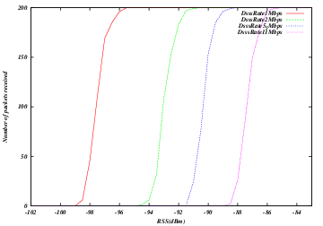
Clear channel (AWGN) error model for 802.11b
Validation results for the 802.11a/g OFDM error model are available in this
technical report. The curves
can be reproduced by running the wifi-ofdm-validation.cc example program
in the examples/wireless directory, and the figure is reproduced below
in Figure Frame error rate (NIST model) for 802.11a/g (OFDM) Wi-Fi.
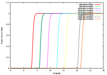
Frame error rate (NIST model) for 802.11a/g (OFDM) Wi-Fi
Similar curves for 802.11n/ac/ax can be obtained by running the wifi-ofdm-ht-validation.cc,
wifi-ofdm-vht-validation.cc and wifi-ofdm-he-validation.cc example programs
in the examples/wireless directory, and the figures are reproduced below
in Figure Frame error rate (NIST model) for 802.11n (HT OFDM) Wi-Fi, Figure Frame error rate (NIST model) for 802.11ac (VHT OFDM) Wi-Fi
and Figure Frame error rate (NIST model) for 802.11ax (HE OFDM) Wi-Fi, respectively.
There is no validation for those curves yet.
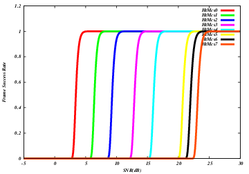
Frame error rate (NIST model) for 802.11n (HT OFDM) Wi-Fi
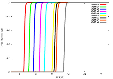
Frame error rate (NIST model) for 802.11ac (VHT OFDM) Wi-Fi
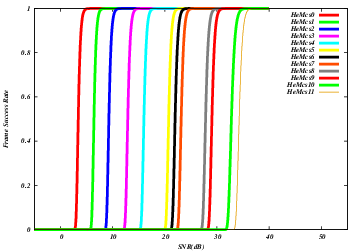
Frame error rate (NIST model) for 802.11ax (HE OFDM) Wi-Fi
MAC validation
Validation of the 802.11 DCF MAC layer has been performed in [baldo2010].
802.11 PCF operation has been verified by running ‘wifi-pcf’ example with PCAP files generation enabled, and observing the frame exchange using Wireshark.
SpectrumWiFiPhy
The SpectrumWifiPhy implementation has been verified to produce equivalent results to the legacy YansWifiPhy by using the saturation and packet error rate programs (described below) and toggling the implementation between the two physical layers.
A basic unit test is provided using injection of hand-crafted packets to a receiving Phy object, controlling the timing and receive power of each packet arrival and checking the reception results. However, most of the testing of this Phy implementation has been performed using example programs described below, and during the course of a (separate) LTE/Wi-Fi coexistence study not documented herein.
Saturation performance
The program examples/wireless/wifi-spectrum-saturation-example.cc
allows user to select either the SpectrumWifiPhy or YansWifiPhy for
saturation tests. The wifiType can be toggled by the argument
'--wifiType=ns3::YansWifiPhy' or --wifiType=ns3::SpectrumWifiPhy'
There isn’t any difference in the output, which is to be expected because this test is more of a test of the DCF than the physical layer.
By default, the program will use the SpectrumWifiPhy and will run for 10 seconds of saturating UDP data, with 802.11n features enabled. It produces this output for the main 802.11n rates (with short and long guard intervals):
wifiType: ns3::SpectrumWifiPhy distance: 1m
index MCS width Rate (Mb/s) Tput (Mb/s) Received
0 0 20 6.5 5.81381 4937
1 1 20 13 11.8266 10043
2 2 20 19.5 17.7935 15110
3 3 20 26 23.7958 20207
4 4 20 39 35.7331 30344
5 5 20 52 47.6174 40436
6 6 20 58.5 53.6102 45525
7 7 20 65 59.5501 50569
...
63 15 40 300 254.902 216459
The above output shows the first 8 (of 32) modes, and last mode, that will be output from the program. The first 8 modes correspond to short guard interval disabled and channel bonding disabled. The subsequent 24 modes run by this program are variations with short guard interval enabled (cases 9-16), and then with channel bonding enabled and short guard first disabled then enabled (cases 17-32). Cases 33-64 repeat the same configurations but for two spatial streams (MIMO abstraction).
When run with the legacy YansWifiPhy, as in ./waf --run "wifi-spectrum-saturation-example --wifiType=ns3::YansWifiPhy", the same output is observed:
wifiType: ns3::YansWifiPhy distance: 1m
index MCS width Rate (Mb/s) Tput (Mb/s) Received
0 0 20 6.5 5.81381 4937
1 1 20 13 11.8266 10043
2 2 20 19.5 17.7935 15110
3 3 20 26 23.7958 20207
...
This is to be expected since YansWifiPhy and SpectrumWifiPhy use the same error rate model in this case.
Packet error rate performance
The program examples/wireless/wifi-spectrum-per-example.cc allows users
to select either SpectrumWifiPhy or YansWifiPhy, as above, and select
the distance between the nodes, and to log the reception statistics and
received SNR (as observed by the WifiPhy::MonitorSnifferRx trace source), using a
Friis propagation loss model. The transmit power is lowered from the default
of 40 mW (16 dBm) to 1 dBm to lower the baseline SNR; the distance between
the nodes can be changed to further change the SNR. By default, it steps
through the same index values as in the saturation example (0 through 31)
for a 50m distance, for 10 seconds of simulation time, producing output such as:
wifiType: ns3::SpectrumWifiPhy distance: 50m; time: 10; TxPower: 1 dBm (1.3 mW)
index MCS Rate (Mb/s) Tput (Mb/s) Received Signal (dBm) Noise (dBm) SNR (dB)
0 0 6.50 5.77 7414 -79.71 -93.97 14.25
1 1 13.00 11.58 14892 -79.71 -93.97 14.25
2 2 19.50 17.39 22358 -79.71 -93.97 14.25
3 3 26.00 22.96 29521 -79.71 -93.97 14.25
4 4 39.00 0.00 0 N/A N/A N/A
5 5 52.00 0.00 0 N/A N/A N/A
6 6 58.50 0.00 0 N/A N/A N/A
7 7 65.00 0.00 0 N/A N/A N/A
As in the above saturation example, running this program with YansWifiPhy will yield identical output.
Interference performance
The program examples/wireless/wifi-spectrum-per-interference.cc is based
on the previous packet error rate example, but copies over the
WaveformGenerator from the unlicensed LTE interferer test, to allow
users to inject a non-Wi-Fi signal (using the --waveformPower argument)
from the command line. Another difference with respect to the packet
error rate example program is that the transmit power is set back to the
default of 40 mW (16 dBm). By default, the interference generator is off,
and the program should behave similarly to the other packet error rate example,
but by adding small
amounts of power (e.g. --waveformPower=0.001), one will start to observe
SNR degradation and frame loss.
Some sample output with default arguments (no interference) is:
./waf --run "wifi-spectrum-per-interference"
wifiType: ns3::SpectrumWifiPhy distance: 50m; time: 10; TxPower: 16 dBm (40 mW)
index MCS Rate (Mb/s) Tput (Mb/s) Received Signal (dBm)Noi+Inf(dBm) SNR (dB)
0 0 6.50 5.77 7414 -64.69 -93.97 29.27
1 1 13.00 11.58 14892 -64.69 -93.97 29.27
2 2 19.50 17.39 22358 -64.69 -93.97 29.27
3 3 26.00 23.23 29875 -64.69 -93.97 29.27
4 4 39.00 34.90 44877 -64.69 -93.97 29.27
5 5 52.00 46.51 59813 -64.69 -93.97 29.27
6 6 58.50 52.39 67374 -64.69 -93.97 29.27
7 7 65.00 58.18 74819 -64.69 -93.97 29.27
...
while a small amount of waveform power will cause frame losses to occur at higher order modulations, due to lower SNR:
./waf --run "wifi-spectrum-per-interference --waveformPower=0.001"
wifiType: ns3::SpectrumWifiPhy distance: 50m; sent: 1000 TxPower: 16 dBm (40 mW)
index MCS Rate (Mb/s) Tput (Mb/s) Received Signal (dBm)Noi+Inf(dBm) SNR (dB)
0 0 6.50 5.77 7414 -64.69 -80.08 15.38
1 1 13.00 11.58 14892 -64.69 -80.08 15.38
2 2 19.50 17.39 22358 -64.69 -80.08 15.38
3 3 26.00 23.23 29873 -64.69 -80.08 15.38
4 4 39.00 0.41 531 -64.69 -80.08 15.38
5 5 52.00 0.00 0 N/A N/A N/A
6 6 58.50 0.00 0 N/A N/A N/A
7 7 65.00 0.00 0 N/A N/A N/A
...
If ns3::YansWifiPhy is selected as the wifiType, the waveform generator will not be enabled because only transmitters of type YansWifiPhy may be connected to a YansWifiChannel.
The interference signal as received by the sending node is typically below the default -62 dBm CCA Mode 1 threshold in this example. If it raises above, the sending node will suppress all transmissions.
Bianchi validation
The program src/wifi/examples/wifi-bianchi.cc allows user to
compare ns-3 simulation results against the Bianchi model
presented in [bianchi2000] and [bianchi2005].
The MATLAB code used to generate the Bianchi model,
as well as the generated outputs, are provided in
the folder src/wifi/examples/reference.
User can regenerate Bianchi results by running
generate_bianchi.m in MATLAB.
By default, the program src/wifi/examples/wifi-bianchi.cc
simulates an 802.11a adhoc ring scenario, with a PHY rate set to
54 Mbit/s, and loop from 5 stations to 50 stations, by a step of
5 stations. It generates a plt file, which allows user to quickly
generate an eps file using gnuplot and vizualize the graph.
./waf --run "wifi-bianchi"
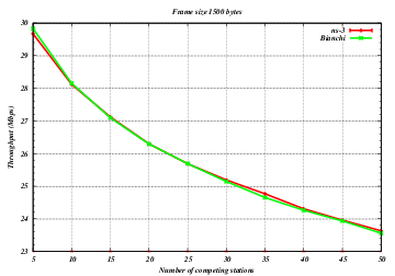
Bianchi throughput validation results for 802.11a 54 Mbps in adhoc configuration
The user has the possibility to select the standard (only 11a, 11b or 11g currently supported), to select the PHY rate (in Mbit/s), as well as to choose between an adhoc or an infrastructure configuration.
When run for 802.11g 6 Mbit/s in infrastucture mode, the output is:
./waf --run "wifi-bianchi --standard=11g --phyRate=6 --duration=500 --infra"
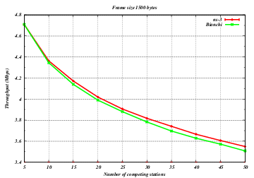
Bianchi throughput validation results for 802.11g 6 Mbps in infrastructure configuration
Multi-user transmissions validation
The implementation of the OFDMA support has been validated against a theoretical model [magrin2021mu] .
A preliminary evaluation of the usage of OFDMA in 802.11ax, in terms of latency in non-saturated conditions, throughput in saturated conditions and transmission range with UL OFDMA, is provided in [avallone2021wcm] .
References
| [ieee80211] | IEEE Std 802.11-2012, Part 11: Wireless LAN Medium Access Control (MAC) and Physical Layer (PHY) Specifications |
| [ieee80211-2016] | IEEE Std 802.11-2016, Part 11: Wireless LAN Medium Access Control (MAC) and Physical Layer (PHY) Specifications |
| [pei80211b] | G. Pei and Tom Henderson, Validation of ns-3 802.11b PHY model |
| [pei80211ofdm] | G. Pei and Tom Henderson, Validation of OFDM error rate model in ns-3 |
| [lacage2006yans] | M. Lacage and T. Henderson, Yet another Network Simulator |
| [Haccoun] | D. Haccoun and G. Begin, High-Rate Punctured Convolutional Codes for Viterbi Sequential Decoding, IEEE Transactions on Communications, Vol. 32, Issue 3, pp.315-319. |
| [Frenger] | Pâl Frenger et al., “Multi-rate Convolutional Codes”. |
| [ji2004sslswn] | Z. Ji, J. Zhou, M. Takai and R. Bagrodia, Scalable simulation of large-scale wireless networks with bounded inaccuracies, in Proc. of the Seventh ACM Symposium on Modeling, Analysis and Simulation of Wireless and Mobile Systems, October 2004. |
| [linuxminstrel] | minstrel linux wireless |
| [lacage2004aarfamrr] | M. Lacage, H. Manshaei, and T. Turletti, IEEE 802.11 rate adaptation: a practical approach, in Proc. 7th ACM International Symposium on Modeling, Analysis and Simulation of Wireless and Mobile Systems, 2004. |
| [kim2006cara] | J. Kim, S. Kim, S. Choi, and D. Qiao, CARA: Collision-Aware Rate Adaptation for IEEE 802.11 WLANs, in Proc. 25th IEEE International Conference on Computer Communications, 2006 |
| [wong2006rraa] | S. Wong, H. Yang, S. Lu, and V. Bharghavan, Robust Rate Adaptation for 802.11 Wireless Networks, in Proc. 12th Annual International Conference on Mobile Computing and Networking, 2006 |
| [maguolo2008aarfcd] | F. Maguolo, M. Lacage, and T. Turletti, Efficient collision detection for auto rate fallback algorithm, in IEEE Symposium on Computers and Communications, 2008 |
| [proakis2001] | J. Proakis, Digital Communications, Wiley, 2001. |
| [miller2003] | L. E. Miller, “Validation of 802.11a/UWB Coexistence Simulation.” Technical Report, October 2003. Available online |
| [ferrari2004] | G. Ferrari and G. Corazza, “Tight bounds and accurate approximations for DQPSK transmission bit error rate”, Electronics Letters, 40(20):1284-85, September 2004. |
| [pursley2009] | M. Pursley and T. Royster, “Properties and performance of the IEEE 802.11b complementary code key signal sets,” IEEE Transactions on Communications, 57(2);440-449, February 2009. |
| [akella2007parf] | A. Akella, G. Judd, S. Seshan, and P. Steenkiste, ‘Self-management in chaotic wireless deployments’, in Wireless Networks, Kluwer Academic Publishers, 2007, 13, 737-755. http://www.cs.odu.edu/~nadeem/classes/cs795-WNS-S13/papers/enter-006.pdf |
| [chevillat2005aparf] | Chevillat, P.; Jelitto, J., and Truong, H. L., ‘Dynamic data rate and transmit power adjustment in IEEE 802.11 wireless LANs’, in International Journal of Wireless Information Networks, Springer, 2005, 12, 123-145. http://www.cs.mun.ca/~yzchen/papers/papers/rate_adaptation/80211_dynamic_rate_power_adjustment_chevillat_j2005.pdf |
| [hepner2015] | C. Hepner, A. Witt, and R. Muenzner, “In depth analysis of the ns-3 physical layer abstraction for WLAN systems and evaluation of its influences on network simulation results”, BW-CAR Symposium on Information and Communication Systems (SInCom) 2015. https://core.ac.uk/download/pdf/75487102.pdf#page=50 |
| [baldo2010] | N. Baldo et al., “Validation of the ns-3 IEEE 802.11 model using the EXTREME testbed”, Proceedings of SIMUTools Conference, March 2010. |
| [lanante2019] | L. Lanante Jr. et al., “Improved Abstraction for Clear Channel Assessment in ns-3 802.11 WLAN Model”, Proceedings of the 2019 Workshop on ns-3, June 2019. |
| [bianchi2000] | G. Bianchi, “Performance analysis of the IEEE 802.11 distributed coordination function”, IEEE Communications Letters, 18(3):535–547, 2000. |
| [bianchi2005] | G. Bianchi and I. Tinnirello. “Remarks on IEEE 802.11 DCF performance analysis”, IEEE Communications Letters, 9(8):765–767, 2005. |
| [patidar2017] | R. Patidar et al., “Link-to-System Mapping for ns-3 Wi-Fi OFDM Error Models”, Proceedings of the Workshop on ns-3, June 2017. https://dl.acm.org/doi/10.1145/3067665.3067671 |
| [erceg2004] | V. Erceg and L. Schumacher and P. Kyritsi, “Tgn channel models”, IEEE 802.11-03/940r4, 2004. |
| [porat2016] | R. Porat et al., “11ax Evaluation Methodology”, IEE P802.11 Wireless LANs, 11-14-0571r3, 2016. |
| [krotov2020rate] | A. Krotov, A. Kiryanov, E. Khorov., Rate Control With Spatial Reuse for Wi-Fi 6 Dense Deployments, IEEE Access, September 2020 |
| [magrin2021mu] | D. Magrin, S. Avallone, S. Roy, and M. Zorzi, ‘Validation of the ns-3 802.11ax OFDMA implementation’, in Proceedings of WNS3 2021. |
| [avallone2021wcm] | S. Avallone, P. Imputato, G. Redieteab, C. Ghosh and S. Roy, “Will OFDMA Improve the Performance of 802.11 WiFi Networks?”, in IEEE Wireless Communications Magazine, DOI: 10.1109/MWC.001.2000332, to appear. |
Wimax NetDevice
This chapter describes the ns-3 WimaxNetDevice and related models. By adding WimaxNetDevice objects to ns-3 nodes, one can create models of 802.16-based networks. Below, we list some more details about what the ns-3 WiMAX models cover but, in summary, the most important features of the ns-3 model are:
- a scalable and realistic physical layer and channel model
- a packet classifier for the IP convergence sublayer
- efficient uplink and downlink schedulers
- support for Multicast and Broadcast Service (MBS), and
- packet tracing functionality
The source code for the WiMAX models lives in the directory
src/wimax.
There have been two academic papers published on this model:
- M.A. Ismail, G. Piro, L.A. Grieco, and T. Turletti, “An Improved IEEE 802.16 WiMAX Module for the NS-3 Simulator”, SIMUTools 2010 Conference, March 2010.
- J. Farooq and T. Turletti, “An IEEE 802.16 WiMAX module for the NS-3 Simulator,” SIMUTools 2009 Conference, March 2009.
Scope of the model
From a MAC perspective, there are two basic modes of operation, that of a
Subscriber Station (SS) or a Base Station (BS). These are implemented as two
subclasses of the base class ns3::NetDevice, class
SubscriberStationNetDevice and class
BaseStationNetDevice. As is typical in ns-3, there is also a
physical layer class WimaxPhy and a channel class
WimaxChannel which serves to hold the references to all of the
attached Phy devices. The main physical layer class is the
SimpleOfdmWimaxChannel class.
Another important aspect of WiMAX is the uplink and downlink scheduler, and there are three primary scheduler types implemented:
- SIMPLE: a simple priority based FCFS scheduler
- RTPS: a real-time polling service (rtPS) scheduler
- MBQOS: a migration-based uplink scheduler
The following additional aspects of the 802.16 specifications, as well as physical layer and channel models, are modelled:
- leverages existing ns-3 wireless propagation loss and delay models, as well as ns-3 mobility models
- Point-to-Multipoint (PMP) mode and the WirelessMAN-OFDM PHY layer
- Initial Ranging
- Service Flow Initialization
- Management Connection
- Transport Initialization
- UGS, rtPS, nrtPS, and BE connections
The following aspects are not presently modelled but would be good topics for future extensions:
- OFDMA PHY layer
- Link adaptation
- Mesh topologies
- ARQ
- ertPS connection
- packet header suppression
Using the Wimax models
The main way that users who write simulation scripts will typically interact with the Wimax models is through the helper API and through the publicly visible attributes of the model.
The helper API is defined in src/wimax/helper/wimax-helper.{cc,h}.
The example src/wimax/examples/wimax-simple.cc contains some basic code that
shows how to set up the model:
switch (schedType)
{
case 0:
scheduler = WimaxHelper::SCHED_TYPE_SIMPLE;
break;
case 1:
scheduler = WimaxHelper::SCHED_TYPE_MBQOS;
break;
case 2:
scheduler = WimaxHelper::SCHED_TYPE_RTPS;
break;
default:
scheduler = WimaxHelper::SCHED_TYPE_SIMPLE;
}
NodeContainer ssNodes;
NodeContainer bsNodes;
ssNodes.Create (2);
bsNodes.Create (1);
WimaxHelper wimax;
NetDeviceContainer ssDevs, bsDevs;
ssDevs = wimax.Install (ssNodes,
WimaxHelper::DEVICE_TYPE_SUBSCRIBER_STATION,
WimaxHelper::SIMPLE_PHY_TYPE_OFDM,
scheduler);
bsDevs = wimax.Install (bsNodes, WimaxHelper::DEVICE_TYPE_BASE_STATION, WimaxHelper::SIMPLE_PHY_TYPE_OFDM, scheduler);
This example shows that there are two subscriber stations and one base station
created. The helper method Install allows the user to specify the scheduler
type, the physical layer type, and the device type.
Different variants of Install are available; for instance, the example
src/wimax/examples/wimax-multicast.cc shows how to specify a non-default channel
or propagation model:
channel = CreateObject<SimpleOfdmWimaxChannel> ();
channel->SetPropagationModel (SimpleOfdmWimaxChannel::COST231_PROPAGATION);
ssDevs = wimax.Install (ssNodes,
WimaxHelper::DEVICE_TYPE_SUBSCRIBER_STATION,
WimaxHelper::SIMPLE_PHY_TYPE_OFDM,
channel,
scheduler);
Ptr<WimaxNetDevice> dev = wimax.Install (bsNodes.Get (0),
WimaxHelper::DEVICE_TYPE_BASE_STATION,
WimaxHelper::SIMPLE_PHY_TYPE_OFDM,
channel,
scheduler);
Mobility is also supported in the same way as in Wifi models; see the
src/wimax/examples/wimax-multicast.cc.
Another important concept in WiMAX is that of a service flow. This is a
unidirectional flow of packets with a set of QoS parameters such as traffic
priority, rate, scheduling type, etc. The base station is responsible for
issuing service flow identifiers and mapping them to WiMAX connections. The
following code from src/wimax/examples/wimax-multicast.cc shows how this is
configured from a helper level:
ServiceFlow MulticastServiceFlow = wimax.CreateServiceFlow (ServiceFlow::SF_DIRECTION_DOWN,
ServiceFlow::SF_TYPE_UGS,
MulticastClassifier);
bs->GetServiceFlowManager ()->AddMulticastServiceFlow (MulticastServiceFlow, WimaxPhy::MODULATION_TYPE_QPSK_12);
Wimax Attributes
The WimaxNetDevice makes heavy use of the ns-3 attributes subsystem for configuration and default value management. Presently, approximately 60 values are stored in this system.
For instance, class ns-3::SimpleOfdmWimaxPhy exports these
attributes:
- NoiseFigure: Loss (dB) in the Signal-to-Noise-Ratio due to non-idealities in the receiver.
- TxPower: Transmission power (dB)
- G: The ratio of CP time to useful time
- txGain: Transmission gain (dB)
- RxGain: Reception gain (dB)
- Nfft: FFT size
- TraceFilePath: Path to the directory containing SNR to block error rate files
For a full list of attributes in these models, consult the Doxygen page that lists all attributes for ns-3.
Wimax Tracing
ns-3 has a sophisticated tracing infrastructure that allows users to hook into existing trace sources, or to define and export new ones.
Many ns-3 users use the built-in Pcap or Ascii tracing, and the WimaxHelper has similar APIs:
AsciiTraceHelper ascii;
WimaxHelper wimax;
wimax.EnablePcap ("wimax-program", false);
wimax.EnableAsciiAll (ascii.CreateFileStream ("wimax-program.tr");
Unlike other helpers, there is also a special EnableAsciiForConnection()
method that limits the ascii tracing to a specific device and connection.
These helpers access the low level trace sources that exist in the WiMAX physical layer, net device, and queue models. Like other ns-3 trace sources, users may hook their own functions to these trace sources if they want to do customized things based on the packet events. See the Doxygen List of trace sources for a complete list of these sources.
Wimax MAC model
The 802.16 model provided in ns-3 attempts to provide an accurate MAC and PHY level implementation of the 802.16 specification with the Point-to-Multipoint (PMP) mode and the WirelessMAN-OFDM PHY layer. The model is mainly composed of three layers:
- The convergence sublayer (CS)
- The MAC CP Common Part Sublayer (MAC-CPS)
- Physical (PHY) layer
The following figure WiMAX architecture shows the relationships of these models.
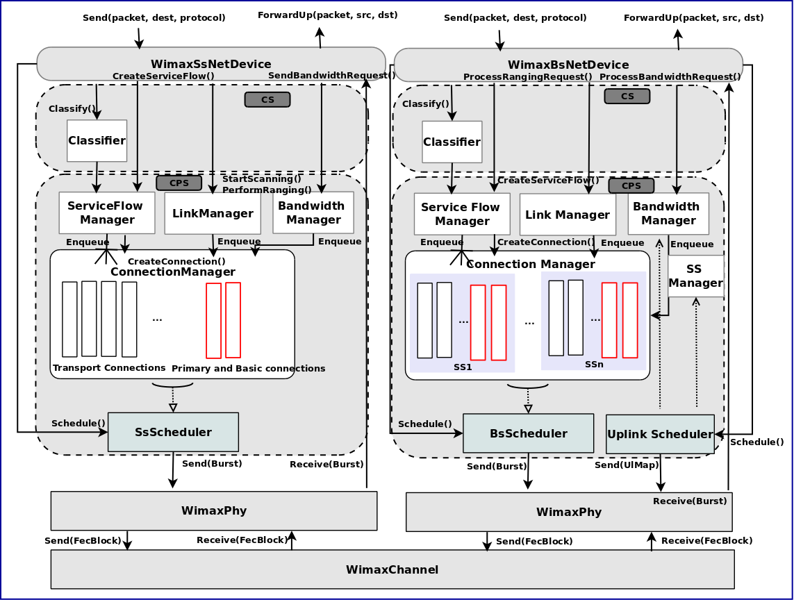
WiMAX architecture
Convergence Sublayer
The Convergence sublayer (CS) provided with this module implements the Packet CS, designed to work with the packet-based protocols at higher layers. The CS is responsible of receiving packet from the higher layer and from peer stations, classifying packets to appropriate connections (or service flows) and processing packets. It keeps a mapping of transport connections to service flows. This enables the MAC CPS identifying the Quality of Service (QoS) parameters associated to a transport connection and ensuring the QoS requirements. The CS currently employs an IP classifier.
IP Packet Classifier
An IP packet classifier is used to map incoming packets to appropriate
connections based on a set of criteria. The classifier maintains a list of
mapping rules which associate an IP flow (src IP address and mask, dst IP
address and mask, src port range, dst port range and protocol) to one of the
service flows. By analyzing the IP and the TCP/UDP headers the classifier will
append the incoming packet (from the upper layer) to the queue of the
appropriate WiMAX connection. Class IpcsClassifier and class
IpcsClassifierRecord implement the classifier module for both SS
and BS
MAC Common Part Sublayer
The MAC Common Part Sublayer (CPS) is the main sublayer of the IEEE 802.16 MAC
and performs the fundamental functions of the MAC. The module implements the
Point-Multi-Point (PMP) mode. In PMP mode BS is responsible of managing
communication among multiple SSs. The key functionalities of the MAC CPS include
framing and addressing, generation of MAC management messages, SS initialization
and registration, service flow management, bandwidth management and scheduling
services. Class WimaxNetDevice represents the MAC layer of a WiMAX
network device. This class extends the class NetDevice of the ns-3
API that provides abstraction of a network device. Class
WimaxNetDevice is further extended by class
BaseStationNetDevice and class
SubscriberStationNetDevice, defining MAC layers of BS and SS,
respectively. Besides these main classes, the key functions of MAC are
distributed to several other classes.
Framing and Management Messages
The module implements a frame as a fixed duration of time, i.e., frame
boundaries are defined with respect to time. Each frame is further subdivided
into downlink (DL) and uplink (UL) subframes. The module implements the Time
Division Duplex (TDD) mode where DL and UL operate on same frequency but are
separated in time. A number of DL and UL bursts are then allocated in DL and UL
subframes, respectively. Since the standard allows sending and receiving bursts
of packets in a given DL or UL burst, the unit of transmission at the MAC layer
is a packet burst. The module implements a special PacketBurst data structure
for this purpose. A packet burst is essentially a list of packets. The BS
downlink and uplink schedulers, implemented by class BSScheduler
and class UplinkScheduler, are responsible of generating DL and UL
subframes, respectively. In the case of DL, the subframe is simulated by
transmitting consecutive bursts (instances PacketBurst). In case of UL, the
subframe is divided, with respect to time, into a number of slots. The bursts
transmitted by the SSs in these slots are then aligned to slot boundaries. The
frame is divided into integer number of symbols and Physical Slots (PS) which
helps in managing bandwidth more effectively. The number of symbols per frame
depends on the underlying implementation of the PHY layer. The size of a DL or
UL burst is specified in units of symbols.
Network Entry and Initialization
The network entry and initialization phase is basically divided into two sub-phases, (1) scanning and synchronization and (2) initial ranging. The entire phase is performed by the LinkManager component of SS and BS. Once an SS wants to join the network, it first scans the downlink frequencies to search for a suitable channel. The search is complete as soon as it detects a PHY frame. The next step is to establish synchronization with the BS. Once SS receives a Downlink-MAP (DL-MAP) message the synchronization phase is complete and it remains synchronized as long as it keeps receiving DL-MAP and Downlink Channel Descriptor (DCD) messages. After the synchronization is established, SS waits for a Uplink Channel Descriptor (UCD) message to acquire uplink channel parameters. Once acquired, the first sub-phase of the network entry and initialization is complete. Once synchronization is achieved, the SS waits for a UL-MAP message to locate a special grant, called initial ranging interval, in the UL subframe. This grant is allocated by the BS Uplink Scheduler at regular intervals. Currently this interval is set to 0.5 ms, however the user is enabled to modify its value from the simulation script.
Connections and Addressing
All communication at the MAC layer is carried in terms of connections. The
standard defines a connection as a unidirectional mapping between the SS and
BS’s MAC entities for the transmission of traffic. The standard defines two
types of connections: management connections for transmitting control messages
and transport connections for data transmission. A connection is identified by a
16-bit Connection Identifier (CID). Class WimaxConnection and
class Cid implement the connection and CID, respectively. Note that
each connection maintains its own transmission queue where packets to transmit
on that connection are queued. The ConnectionManager component of BS is
responsible of creating and managing connections for all SSs.
The two key management connections defined by the standard, namely the Basic and Primary management connections, are created and allocated to the SS during the ranging process. Basic connection plays an important role throughout the operation of SS also because all (unicast) DL and UL grants are directed towards SS’s Basic CID. In addition to management connections, an SS may have one or more transport connections to send data packets. The Connection Manager component of SS manages the connections associated to SS. As defined by the standard, a management connection is bidirectional, i.e., a pair of downlink and uplink connections is represented by the same CID. This feature is implemented in a way that one connection (in DL direction) is created by the BS and upon receiving the CID the SS then creates an identical connection (in UL direction) with the same CID.
Scheduling Services
The module supports the four scheduling services defined by the 802.16-2004 standard:
- Unsolicited Grant Service (UGS)
- Real-Time Polling Services (rtPS)
- Non Real-Time Polling Services (nrtPS)
- Best Effort (BE)
These scheduling services behave differently with respect to how they request bandwidth as well as how the it is granted. Each service flow is associated to exactly one scheduling service, and the QoS parameter set associated to a service flow actually defines the scheduling service it belongs to. When a service flow is created the UplinkScheduler calculates necessary parameters such as grant size and grant interval based on QoS parameters associated to it.
WiMAX Uplink Scheduler Model
Uplink Scheduler at the BS decides which of the SSs will be assigned uplink allocations based on the QoS parameters associated to a service flow (or scheduling service) and bandwidth requests from the SSs. Uplink scheduler together with Bandwidth Manager implements the complete scheduling service functionality. The standard defines up to four scheduling services (BE, UGS, rtPS, nrtPS) for applications with different types of QoS requirements. The service flows of these scheduling services behave differently with respect to how they request for bandwidth as well as how the bandwidth is granted. The module supports all four scheduling services. Each service flow is associated to exactly one transport connection and one scheduling service. The QoS parameters associated to a service flow actually define the scheduling service it belongs to. Standard QoS parameters for UGS, rtPS, nrtPS and BE services, as specified in Tables 111a to 111d of the 802.16e amendment, are supported. When a service flow is created the uplink scheduler calculates necessary parameters such as grant size and allocation interval based on QoS parameters associated to it. The current WiMAX module provides three different versions of schedulers.
- The first one is a simple priority-based First Come First Serve (FCFS). For
the real-time services (UGS and rtPS) the BS then allocates grants/polls on
regular basis based on the calculated interval. For the non real-time services
(nrtPS and BE) only minimum reserved bandwidth is guaranteed if available
after servicing real-time flows. Note that not all of these parameters are
utilized by the uplink scheduler. Also note that currently only service flow
with fixed-size packet size are supported, as currently set up in simulation
scenario with OnOff application of fixed packet size. This scheduler is
implemented by class
BSSchedulerSimpleand classUplinkSchedulerSimple. - The second one is similar to first scheduler except by rtPS service flow. All
rtPS Connections are able to transmit all packet in the queue according to the
available bandwidth. The bandwidth saturation control has been implemented to
redistribute the effective available bandwidth to all rtPS that have at least
one packet to transmit. The remaining bandwidth is allocated to nrtPS and BE
Connections. This scheduler is implemented by class
BSSchedulerRtpsand classUplinkSchedulerRtps. - The third one is a Migration-based Quality of Service uplink scheduler This
uplink scheduler uses three queues, the low priority queue, the intermediate
queue and the high priority queue. The scheduler serves the requests in
strict priority order from the high priority queue to the low priority queue.
The low priority queue stores the bandwidth requests of the BE service flow.
The intermediate queue holds bandwidth requests sent by rtPS and by nrtPS
connections. rtPS and nrtPS requests can migrate to the high priority queue to
guarantee that their QoS requirements are met. Besides the requests migrated
from the intermediate queue, the high priority queue stores periodic grants
and unicast request opportunities that must be scheduled in the following
frame. To guarantee the maximum delay requirement, the BS assigns a deadline
to each rtPS bandwidth request in the intermediate queue. The minimum
bandwidth requirement of both rtPS and nrtPS connections is guaranteed over a
window of duration T. This scheduler is implemented by class
UplinkSchedulerMBQoS.
WiMAX Outbound Schedulers Model
Besides the uplink scheduler these are the outbound schedulers at BS and SS side (BSScheduler and SSScheduler). The outbound schedulers decide which of the packets from the outbound queues will be transmitted in a given allocation. The outbound scheduler at the BS schedules the downlink traffic, i.e., packets to be transmitted to the SSs in the downlink subframe. Similarly the outbound scheduler at a SS schedules the packet to be transmitted in the uplink allocation assigned to that SS in the uplink subframe. All three schedulers have been implemented to work as FCFS scheduler, as they allocate grants starting from highest priority scheduling service to the lower priority one (UGS> rtPS> nrtPS> BE). The standard does not suggest any scheduling algorithm and instead leaves this decision up to the manufacturers. Of course more sophisticated algorithms can be added later if required.
WimaxChannel and WimaxPhy models
The module implements the Wireless MAN OFDM PHY specifications as the more relevant for implementation as it is the schema chosen by the WiMAX Forum. This specification is designed for non-light-of-sight (NLOS) including fixed and mobile broadband wireless access. The proposed model uses a 256 FFT processor, with 192 data subcarriers. It supports all the seven modulation and coding schemes specified by Wireless MAN-OFDM. It is composed of two parts: the channel model and the physical model.
Channel model
The channel model we propose is implemented by the class
SimpleOFDMWimaxChannel which extends the class
wimaxchannel. The channel entity has a private structure named
m_phyList which handles all the physical devices connected to it. When a
physical device sends a packet (FEC Block) to the channel, the channel handles
the packet, and then for each physical device connected to it, it calculates the
propagation delay, the path loss according to a given propagation model and
eventually forwards the packet to the receiver device. The channel class uses
the method GetDistanceFrom() to calculate the distance between two physical
entities according to their 3D coordinates. The delay is
computed as delay = distance/C, where C is the speed of the light.
Physical model
The physical layer performs two main operations: (i) It receives a burst from a channel and forwards it to the MAC layer, (ii) it receives a burst from the MAC layer and transmits it on the channel. In order to reduce the simulation complexity of the WiMAX physical layer, we have chosen to model offline part of the physical layer. More specifically we have developed an OFDM simulator to generate trace files used by the reception process to evaluate if a FEC block can be correctly decoded or not.
Transmission Process: A burst is a set of WiMAX MAC PDUs. At the sending process, a burst is converted into bit-streams and then split into smaller FEC blocks which are then sent to the channel with a power equal P_tx.
Reception Process: The reception process includes the following operations:
- Receive a FEC block from the channel.
- Calculate the noise level.
- Estimate the signal to noise ratio (SNR) with the following formula.
- Determine if a FEC block can be correctly decoded.
- Concatenate received FEC blocks to reconstruct the original burst.
- Forward the burst to the upper layer.
The developed process to evaluate if a FEC block can be correctly received or not uses pre-generated traces. The trace files are generated by an external OFDM simulator (described later). A class named SNRToBlockErrorRateManager handles a repository containing seven trace files (one for each modulation and coding scheme). A repository is specific for a particular channel model.
A trace file is made of 6 columns. The first column provides the SNR value (1), whereas the other columns give respectively the bit error rate BER (2), the block error rate BlcER(3), the standard deviation on BlcER, and the confidence interval (4 and 5). These trace files are loaded into memory by the SNRToBlockErrorRateManager entity at the beginning of the simulation.
Currently, The first process uses the first and third columns to determine if a FEC block is correctly received. When the physical layer receives a packet with an SNR equal to SNR_rx, it asks the SNRToBlockErrorRateManager to return the corresponding block error rate BlcER. A random number RAND between 0 and 1 is then generated. If RAND is greater than BlcER, then the block is correctly received, otherwise the block is considered erroneous and is ignored.
The module provides defaults SNR to block error rate traces in default-traces.h. The traces have been generated by an External WiMAX OFDM simulator. The simulator is based on an external mathematics and signal processing library IT++ and includes : a random block generator, a Reed Solomon (RS) coder, a convolutional coder, an interleaver, a 256 FFT-based OFDM modulator, a multi-path channel simulator and an equalizer. The multipath channel is simulated using the TDL_channel class of the IT++ library.
Users can configure the module to use their own traces generated by another OFDM simulator or ideally by performing experiments in real environment. For this purpose, a path to a repository containing trace files should be provided. If no repository is provided the traces form default-traces.h will be loaded. A valid repository should contain 7 files, one for each modulation and coding scheme.
The names of the files should respect the following format: modulation0.txt for modulation 0, modulation1.txt for modulation 1 and so on… The file format should be as follows:
SNR_value1 BER Blc_ER STANDARD_DEVIATION CONFIDENCE_INTERVAL1 CONFIDENCE_INTERVAL2
SNR_value2 BER Blc_ER STANDARD_DEVIATION CONFIDENCE_INTERVAL1 CONFIDENCE_INTERVAL2
... ... ... ... ... ...
... ... ... ... ... ...