HOWTO get ns-3 to detect steady-state times in your data: Difference between revisions
No edit summary |
No edit summary |
||
| (7 intermediate revisions by the same user not shown) | |||
| Line 42: | Line 42: | ||
** Algorithm: Standardized time series methods for steady-state detection. | ** Algorithm: Standardized time series methods for steady-state detection. | ||
** Reason: Single-replicate algorithm. | ** Reason: Single-replicate algorithm. | ||
* '''Nakayama, M. K. (1994)'''. Two-stage Stopping Procedures Based on Standardized Time Series. ''Management Science'' 40:1189–1206. | * '''Nakayama, M. K. (1994)'''. Two-stage Stopping Procedures Based on Standardized Time Series. ''Management Science'' 40:1189–1206. | ||
| Line 65: | Line 59: | ||
** Reason: Glynn and Whitt consider several so-called sequential procedures. | ** Reason: Glynn and Whitt consider several so-called sequential procedures. | ||
== Rejected | == Algorithms Rejected without Trying == | ||
* Multiple (3) steady-state algorithms in an Excel based tool. | |||
** '''Robinson, Stewart (2005)'''. Automated Analysis of Simulation Output Data. ''Proceedings of the 2005 Winter Simulation Conference''. | |||
** Summary: Paper describes an Excel based semi-automated tool that calls SIMUL8. | |||
** Advantages: Automated methods. Describes batch method which works for single seed values. | |||
** Disadvantages: Based on Excel and SIMUL8, which means can't be called from ns-3. | |||
** Note: Has equations for an automated version of Welch's visual method. | |||
** Note: Describes how to automate the batch mean method. See Robinson (2002) in Rejected Algorithms section for equations for batch mean method. | |||
** Note: Describes how to automate the MSER-5 method. | |||
* Schruben's test applied after 25 crossings of the running Mean | |||
** '''Pawlikowski, K, (1990)''', Steady State Simulation of Queueing Processes: a Survey of Problems and Solutions, ''ACM Computing Surveys'', 22, June 1990, 123-170. | |||
** '''McNickle, D., Ewing, G.C., and Pawlikowski, K.. (2007)'''. Transient Deletion And The Quality Of Sequential Steady-State Simulation, ''Proceedings 21st European Conference on Modelling and Simulation''. | |||
*** In this reference, they say: "Details of our sequential implementation of a Schruben-based method can be found in Section 3 of Pawlikowski (1990)." | |||
*** In this reference, they say that the Akaroa2 simulator requires 25 crossings of the running mean of the values before it performs its Schruben’s test. | |||
*** In this reference, they say: "Sequential Spectral Analysis, a modification of the method proposed by Heidelberger and Welch (1981) and specified in Pawlikowski (1990), was used to estimate the confidence interval width. We have found that this method gives accurate confidence intervals, especially for highly correlated data, such as waiting times in highly loaded queues (Ewing, McNickle and Pawlikowski 2002, McNickle, Pawlikowski, and Ewing, 2004). | |||
** '''Hoad, K., Robinson, S., & Davies, R. (2008)'''. Automating Warm-Up Length Estimation. ''Proceedings of the 2008 Winter Simulation Conference'', 532–540. | |||
*** In this reference, they say: "For example, the crossing-of-the-mean rule (Fishman 1973, Wilson and Pritsker 1978a, 1978b) was heavily criticised in the literature for being extremely sensitive to the selection of its main parameter, which was system-dependent, and misspecification of which caused significant over or under-estimation of the warm-up length (Pawlikowski 1990)." | |||
*** In this reference, they call Pawlikowski (1990), the "Goodness-Of-Fit method", and they say: "Both the goodness of fit method and Kimbler’s double exponential smoothing method consistently and severely underestimated the truncation point and were therefore rejected." | |||
** Algorithm: Standardized time series methods for steady-state detection. | |||
** Reason: Single-replicate algorithm. | |||
* Statistical Process Control (SPC) Approach | * Statistical Process Control (SPC) Approach | ||
| Line 76: | Line 91: | ||
** Note: Has equations for batch mean method, which works for single seeds. | ** Note: Has equations for batch mean method, which works for single seeds. | ||
== Algorithms Rejected after Trying == | |||
== Algorithms | |||
* Mean Squared Error Reduction (MSER-5) method applied after 25 crossings of the running Mean | * Mean Squared Error Reduction (MSER-5) method applied after 25 crossings of the running Mean | ||
| Line 99: | Line 105: | ||
** Note: The MSER-5 method alone was saying the system was in steady-state with as few as 2 data values. | ** Note: The MSER-5 method alone was saying the system was in steady-state with as few as 2 data values. | ||
** Note: My code now requires 25 mean crossings before the MSER-5 method is tried, which means the system is in steady-state and which is the situation the MSER-5 method was intended to work with. | ** Note: My code now requires 25 mean crossings before the MSER-5 method is tried, which means the system is in steady-state and which is the situation the MSER-5 method was intended to work with. | ||
** Note: The following plot shows a simulated data set with an exponential bias along with the steady-state time that my implementation of the MSER-5 algorithm (after 25 mean crossings) is currently returning. The plot also shows vertical lines where the steady-state time is and where the 25th mean crossing takes place. | ** Note: The following plot shows a simulated data set with an exponential bias along with the steady-state time that my implementation of the MSER-5 algorithm (after 25 mean crossings) is currently returning. The plot also shows vertical lines where the steady-state time is and where the 25th mean crossing takes place. [[Image:steady-state-detector-test-exponential-bias.png|540px|center|Simulated data set with steady-state time.]] | ||
[[Image:steady-state-detector-test-exponential-bias.png|540px|center|Simulated data set with steady-state time.]] | |||
** Note: My code seems to be giving a better steady-state time than just using the MSER-5 for the first 1,000 points, but it did require almost 2,000 points to get 25 mean crossings. | ** Note: My code seems to be giving a better steady-state time than just using the MSER-5 for the first 1,000 points, but it did require almost 2,000 points to get 25 mean crossings. | ||
** Note: The following plot shows a simulated data set with a linearly increasing bias along with the steady-state time that my implementation of the MSER-5 algorithm (after 25 mean crossings) is currently returning. The plot also shows vertical lines where the steady-state time is and where the 25th mean crossing takes place. [[Image:steady-state-detector-test-linearly-increasing-bias.png|540px|center|Simulated data set with steady-state time.]] | |||
** '''Note: The problem with the MSER-5 algorithm is that the data set with a linearly increasing bias in the above plot does NOT have a steady-state time, and so the algorithm should NOT be finding one. So, the MSER-5algorithm is being REJECTED.''' | |||
** '''Hoad, K., Robinson, S., & Davies, R. (2008)'''. Automating Warm-Up Length Estimation. ''Proceedings of the 2008 Winter Simulation Conference'', 532–540. | |||
*** In this reference, they say: "For example, the crossing-of-the-mean rule (Fishman 1973, Wilson and Pritsker 1978a, 1978b) was heavily criticised in the literature for being extremely sensitive to the selection of its main parameter, which was system-dependent, and misspecification of which caused significant over or under-estimation of the warm-up length (Pawlikowski 1990)." | |||
== Algorithms Currently Trying == | |||
=== Batch Means (BM) Test === | |||
==== Background ==== | |||
* '''White, K., Cobb, M., & Spratt, S. (2000)'''. A Comparison of Five Steady-state Truncation Heuristics for Simulation. ''Proceedings of the 32nd Winter Simulation Conference (WSC '00)'', 755–760. | |||
** In this reference, they say: "Cash, et al. (1992), Nelson (1992), and Goldsman, et al. (1994), propose a family of related tests for detecting the presence of bias in an output series. These tests generalize and extend the earlier work Schruben (1982) and Schruben, et al. (1983)." | |||
* '''Cash, C.R., Dippold, D.G., Nelson, B.L., Pollard, W.P., and Long, J.M. (1992)'''. Evaluation of Tests for Initial-condition Bias. ''Proceedings of the 1992 Winter Simulation Conference'', 577-585. | |||
* Algorithm: Bias detection test. | |||
* Reason: Steady-state detection method can detect if not in steady-state (unlike MSER-5). | |||
* Reason: Single-replicate algorithm. | |||
==== Simulated Test Data ==== | |||
* Note: The following plot shows a simulated data set '''(with 2,000 data values)''' that has an exponential bias along with the steady-state times that my implementations of the Batch Mean (BM) algorithm and the MSER-5 algrothm are currently returning. The plot also shows vertical lines where the steady-state times are. [[Image:steady-state-detector-test-exponential-bias-data-values.png|540px|center|Simulated data set with steady-state time.]] | |||
* Note: The BM method is giving a steady-state time after steady-state has been reached, which would cause it to delete more values than the MSER-5 method. | |||
* Note: The following plot shows the steady-state times calculated as a function of the number of data values for the simulated data set with an exponential bias. [[Image:steady-state-detector-test-exponential-bias-steady-state-times-vs-number-of-values.png|540px|center|Simulated data set with steady-state time.]] | |||
* Note: The above figure shows a problem with the BM method that data sets with fewer values than are required for steady-state (to the left of the blue line) are being called steady-state by the algorithm and giving steady-state times much less than the true steady-state time (the green line). | |||
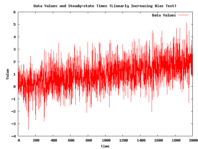
* Note: The following plot shows a simulated data set '''(with 2,000 data values)''' that has a linearly increasing bias. My implementation of the Batch Mean (BM) algorithm did not find a steady-state time for this number of data values. [[Image:steady-state-detector-test-linearly-increasing-bias-data-values.png|540px|center|Simulated data set with steady-state time.]] | |||
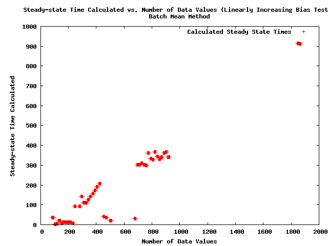
* Note: The following plot shows the steady-state times calculated as a function of the number of data values for the simulated data set with a linearly increasing bias. [[Image:steady-state-detector-test-linearly-increasing-bias-steady-state-times-vs-number-of-values.png|540px|center|Simulated data set with steady-state time.]] | |||
* Note: The above figure shows a problem with the BM method that data sets that are not at steady-state, i.e. all of the data values in this data set, are being called steady-state by the algorithm. | |||
* '''Note: Because the Batch Mean (BM) algorithm is detecting steady-state for data sets that are not in steady-state, it is being REJECTED.''' | |||
==== MANET Routing ExampLe Data ==== | |||
* Note: There are now 2 steady-state detectors in the SAFE MANET example: | |||
** Packets Received | |||
** Receive Rate | |||
* Note: Although the plots have different numerical values for packets-received and receive-rate, they do have the same shape, which means the 2 quantities appear to be linearly related. | |||
* Note: I made the example run for 1000 seconds so that it would be in steady-state. | |||
* Note: The attached plots make it look like the MSER-5 method works well for simulations like this that have achieved steady-state. | |||
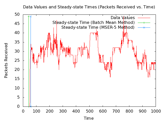
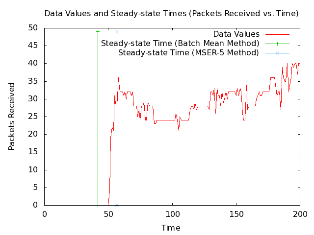
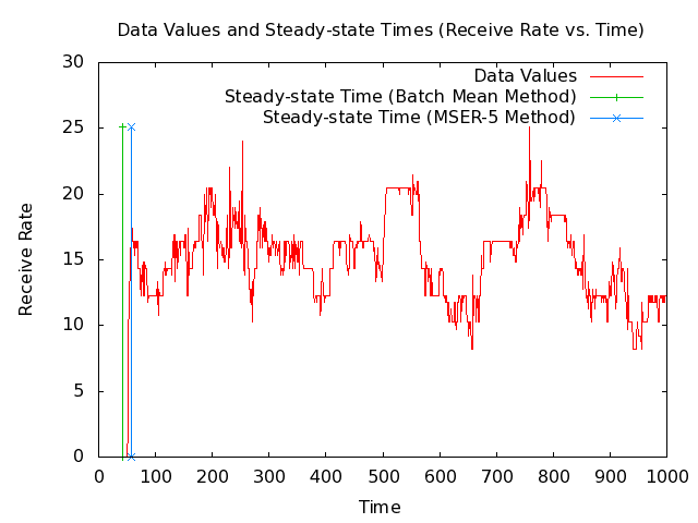
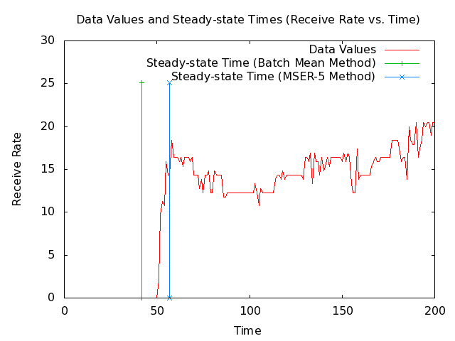
* Note: The following 2 plots show 1000 and 200 seconds from the MANET packets-received data set along with the steady-state times that my implementations of the Batch Mean (BM) algorithm and the MSER-5 algrothm are currently returning. The plots also show vertical lines where the steady-state times are. [[Image:Manet-routing-safe-steady-state-detector-packets-received-data-values-1000-seconds.png|540px|center|SAFE MANET example packets-received data set with steady-state time.]] [[Image:Manet-routing-safe-steady-state-detector-packets-received-data-values-200-seconds.png|540px|center|SAFE MANET example packets-received data set with steady-state time.]] | |||
* Note: The BM method is giving a steady-state time before steady-state has been reached, which would cause it to include unwanted values that the MSER-5 method does not. | |||
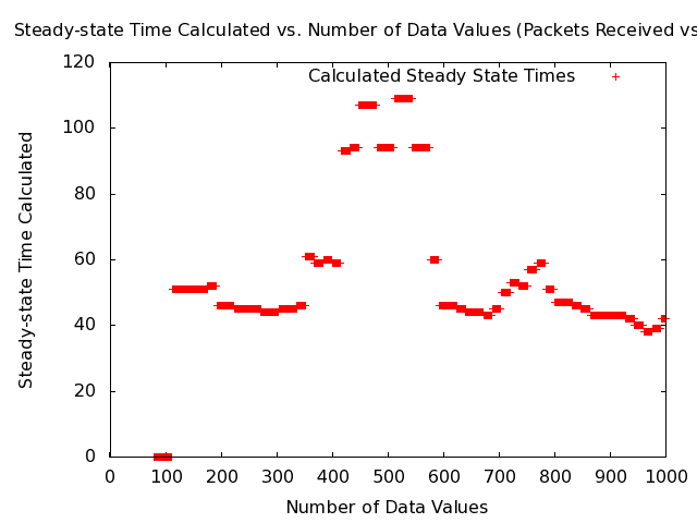
* Note: The following plot shows the steady-state times calculated as a function of the number of data values for the MANET packets-received data set. [[Image:Manet-routing-safe-steady-state-detector-packets-received-steady-state-times-vs-number-of-values-1000-seconds.png|540px|center|Simulated data set with steady-state time.]] | |||
* Note: The above figure shows a problem with the BM method that data sets with fewer values than are required for steady-state for times up to around 120 seconds are being called steady-state by the algorithm and giving steady-state times much less than the true steady-state time, which is around 60 seconds. | |||
* Note: The following 2 plots show 1000 and 200 seconds from the MANET receive-rate data set along with the steady-state times that my implementations of the Batch Mean (BM) algorithm and the MSER-5 algrothm are currently returning. The plots also show vertical lines where the steady-state times are. [[Image:Manet-routing-safe-steady-state-detector-receive-rate-data-values-1000-seconds.png|540px|center|SAFE MANET example receive-rate data set with steady-state time.]] [[Image:Manet-routing-safe-steady-state-detector-receive-rate-data-values-200-seconds.png|540px|center|SAFE MANET example receive-rate data set with steady-state time.]] | |||
* Note: The BM method is giving a steady-state time before steady-state has been reached, which would cause it to include unwanted values that the MSER-5 method does not. | |||
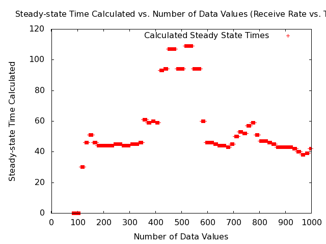
* Note: The following plot shows the steady-state times calculated as a function of the number of data values for the MANET receive-rate data set. [[Image:Manet-routing-safe-steady-state-detector-receive-rate-steady-state-times-vs-number-of-values-1000-seconds.png|540px|center|Simulated data set with steady-state time.]] | |||
* Note: The above figure shows a problem with the BM method that data sets with fewer values than are required for steady-state for times up to around 120 seconds are being called steady-state by the algorithm and giving steady-state times much less than the true steady-state time, which is around 60 seconds. | |||
* '''Note: Because the Batch Mean (BM) algorithm is detecting steady-state for data sets that are not in steady-state, it is being REJECTED.''' | |||
==== Conclusion ==== | |||
'''A more robust steady-state detection algorithm than the Batch Mean (BM) algorithm should be implemented that will then be coupled with the MSER-5 method that appears to work well for simulations once they have achieved steady-state.''' | |||
== Algorithms to Try (In order that they should be tried) == | == Algorithms to Try (In order that they should be tried) == | ||
Latest revision as of 23:23, 3 February 2012
Framework
Steady-state detectors
The architecture of SAFE provides for the use of mechanisms to determine when metrics estimated through simulation have reached steady-state. Although well known, the initialization bias problem hasn't been addressed satisfactorily in the domain of network simulation. Few published research studies have taken steps to exclude samples generated during model transients from their statistical data analysis. Among other researchers who have identified the relevance of initialization bias in network simulation, "Perrone, Yuan, and Nicol [2003]":http://redmine.eg.bucknell.edu/safe/attachments/16/perrone2003.pdf report the significance of avoiding the use of samples from transient in the computation of statistical estimators for metrics of interest.
SAFE enables one to hook up a source of samples to an analysis module, which determines on its own whether the sample data is "in transient" or in steady-state.
The development of _steady-state detectors_ for SAFE is looking at a broad range of publications that will culminate in the identification of sound data analysis methodology. SAFE will use the information provided by steady-state detectors to implement data deletion in the samples collected thereby avoiding initialization bias.
Current Stage of Development
This work is at an investigation stage. We are currently going through the literature to identify algorithms that will be suitable for use in SAFE steady-state detectors.
Projected Milestones
- Literature search and evaluation: June 8-14, 2011
- First implementation: June 15-30, 2011
- Evaluation of implementation against synthetic data generator: July 1-20, 2011
References to Get
- Law, A. M. (2007). Simulation Modeling and Analysis. 4th ed. New York: McGraw-Hill.
- Algorithm: Batch means for steady-state detection. (See pp. 528–529.)
- Reason: An overview of simulation.
- Reason: An overview of single-replicate techniques.
- Reason: Single-replicate algorithm.
- Anderson, T. W. (1994). The Statistical Analysis of Time Series. New York: Wiley.
- Algorithm: Spectral methods for steady-state detection.
- Reason: Single-replicate algorithm.
- Schruben, L. (1982). Detecting Initialisation Bias in Simulation Output. Operations Research, 30(3), 569-590.
- Algorithm: Standardized time series methods for steady-state detection.
- Reason: Single-replicate algorithm.
- Schruben, L. W. (1983). Confidence Interval Estimation using Standardized Time Series. Operations Research 31:1090–1108.
- Algorithm: Standardized time series methods for confidence intervals.
- Reason: Single-replicate algorithm.
- Schruben, L., Singh, H., and Tierney, L. (1983). Optimal Tests for Initialisation Bias in Simulation Output. Operations Research, 31( 6), 1167-1178.
- Algorithm: Standardized time series methods for steady-state detection.
- Reason: Single-replicate algorithm.
- Nakayama, M. K. (1994). Two-stage Stopping Procedures Based on Standardized Time Series. Management Science 40:1189–1206.
- Algorithm: Standardized time series methods for confidence intervals.
- Reason: Might be a single-replicate algorithm.
- Reason: Confidence interval algorithm.
- Reason: Nakayama presents two-stage procedures for obtaining fixed-width confidence intervals using standardized time series methods.
- Pawlikowski, K., McNickle, D., and Ewing, G. (1998). Coverage of Confidence Intervals from Sequential Steady-state Simulation, Simulation Practice and Theory, 6:255-267.
- Algorithm: Confidence intervals.
- Reason: Confidence interval algorithm.
- Glynn, P. W., and W. Whitt. (1992). The Asymptotic Validity of Sequential Stopping Rules in Stochastic Simulations. Annals of Applied Probability 2:180–198.
- Algorithm: Sequential procedures for confidence intervals.
- Reason: Might be a single-replicate algorithm.
- Reason: Confidence interval algorithm.
- Reason: Glynn and Whitt consider several so-called sequential procedures.
Algorithms Rejected without Trying
- Multiple (3) steady-state algorithms in an Excel based tool.
- Robinson, Stewart (2005). Automated Analysis of Simulation Output Data. Proceedings of the 2005 Winter Simulation Conference.
- Summary: Paper describes an Excel based semi-automated tool that calls SIMUL8.
- Advantages: Automated methods. Describes batch method which works for single seed values.
- Disadvantages: Based on Excel and SIMUL8, which means can't be called from ns-3.
- Note: Has equations for an automated version of Welch's visual method.
- Note: Describes how to automate the batch mean method. See Robinson (2002) in Rejected Algorithms section for equations for batch mean method.
- Note: Describes how to automate the MSER-5 method.
- Schruben's test applied after 25 crossings of the running Mean
- Pawlikowski, K, (1990), Steady State Simulation of Queueing Processes: a Survey of Problems and Solutions, ACM Computing Surveys, 22, June 1990, 123-170.
- McNickle, D., Ewing, G.C., and Pawlikowski, K.. (2007). Transient Deletion And The Quality Of Sequential Steady-State Simulation, Proceedings 21st European Conference on Modelling and Simulation.
- In this reference, they say: "Details of our sequential implementation of a Schruben-based method can be found in Section 3 of Pawlikowski (1990)."
- In this reference, they say that the Akaroa2 simulator requires 25 crossings of the running mean of the values before it performs its Schruben’s test.
- In this reference, they say: "Sequential Spectral Analysis, a modification of the method proposed by Heidelberger and Welch (1981) and specified in Pawlikowski (1990), was used to estimate the confidence interval width. We have found that this method gives accurate confidence intervals, especially for highly correlated data, such as waiting times in highly loaded queues (Ewing, McNickle and Pawlikowski 2002, McNickle, Pawlikowski, and Ewing, 2004).
- Hoad, K., Robinson, S., & Davies, R. (2008). Automating Warm-Up Length Estimation. Proceedings of the 2008 Winter Simulation Conference, 532–540.
- In this reference, they say: "For example, the crossing-of-the-mean rule (Fishman 1973, Wilson and Pritsker 1978a, 1978b) was heavily criticised in the literature for being extremely sensitive to the selection of its main parameter, which was system-dependent, and misspecification of which caused significant over or under-estimation of the warm-up length (Pawlikowski 1990)."
- In this reference, they call Pawlikowski (1990), the "Goodness-Of-Fit method", and they say: "Both the goodness of fit method and Kimbler’s double exponential smoothing method consistently and severely underestimated the truncation point and were therefore rejected."
- Algorithm: Standardized time series methods for steady-state detection.
- Reason: Single-replicate algorithm.
- Statistical Process Control (SPC) Approach
- Robinson, Stewart (2002). A Statistical Process Control Approach for Estimating the Warm-Up Period. Proceedings of the 2002 Winter Simulation Conference.
- Summary: 2 stage method:
- Stage 1: has multiple replications.
- Stage 2: has single seed.
- Advantages: Works with a single seed value for stage 2.
- Disadvantages: Requires visual inspection of final results and initial preliminary runs from Stage 1.
- Note: Has equations for batch mean method, which works for single seeds.
Algorithms Rejected after Trying
- Mean Squared Error Reduction (MSER-5) method applied after 25 crossings of the running Mean
- White, K.P. and Robinson, S. (2010). The Problem of the Initial Transient (Again) or Why MSER Works. Journal of Simulation 4, 268-272.
- Franklin, W.W. and White, K.P. (2008). Stationarity Tests and MSER-5: Exploring the Intuition behind Mean-Squared-Error-Reduction in Detecting and Correcting Initialization Bias. Proceedings of the 2008 Winter Simulation Conference.
- White, K.P. and Cobb, M.J. (2000). A Comparison of Five Steady-State Truncation Heuristics for Simulation. Proceedings of the 2000 Winter Simulation Conference.
- This reference showed that the MSER-5 method performed the best of the five methods tried.
- McNickle, D., Ewing, G.C., and Pawlikowski, K.. (2007). Transient Deletion And The Quality Of Sequential Steady-State Simulation, Proceedings 21st European Conference on Modelling and Simulation.
- In this reference, they say that the Akaroa2 simulator requires 25 crossings of the running mean of the values before it performs its Schruben’s test.
- Summary: MSER-5 tries to reduce the mean squared error.
- Advantages: Single-replicate algorithm.
- Disadvantages:
- Note: The MSER-5 method alone was saying the system was in steady-state with as few as 2 data values.
- Note: My code now requires 25 mean crossings before the MSER-5 method is tried, which means the system is in steady-state and which is the situation the MSER-5 method was intended to work with.
- Note: The following plot shows a simulated data set with an exponential bias along with the steady-state time that my implementation of the MSER-5 algorithm (after 25 mean crossings) is currently returning. The plot also shows vertical lines where the steady-state time is and where the 25th mean crossing takes place.
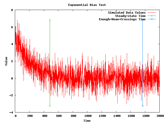
- Note: My code seems to be giving a better steady-state time than just using the MSER-5 for the first 1,000 points, but it did require almost 2,000 points to get 25 mean crossings.
- Note: The following plot shows a simulated data set with a linearly increasing bias along with the steady-state time that my implementation of the MSER-5 algorithm (after 25 mean crossings) is currently returning. The plot also shows vertical lines where the steady-state time is and where the 25th mean crossing takes place.
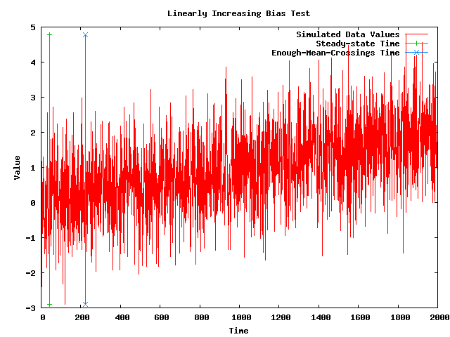
- Note: The problem with the MSER-5 algorithm is that the data set with a linearly increasing bias in the above plot does NOT have a steady-state time, and so the algorithm should NOT be finding one. So, the MSER-5algorithm is being REJECTED.
- Hoad, K., Robinson, S., & Davies, R. (2008). Automating Warm-Up Length Estimation. Proceedings of the 2008 Winter Simulation Conference, 532–540.
- In this reference, they say: "For example, the crossing-of-the-mean rule (Fishman 1973, Wilson and Pritsker 1978a, 1978b) was heavily criticised in the literature for being extremely sensitive to the selection of its main parameter, which was system-dependent, and misspecification of which caused significant over or under-estimation of the warm-up length (Pawlikowski 1990)."


Algorithms Currently Trying
Batch Means (BM) Test
Background
- White, K., Cobb, M., & Spratt, S. (2000). A Comparison of Five Steady-state Truncation Heuristics for Simulation. Proceedings of the 32nd Winter Simulation Conference (WSC '00), 755–760.
- In this reference, they say: "Cash, et al. (1992), Nelson (1992), and Goldsman, et al. (1994), propose a family of related tests for detecting the presence of bias in an output series. These tests generalize and extend the earlier work Schruben (1982) and Schruben, et al. (1983)."
- Cash, C.R., Dippold, D.G., Nelson, B.L., Pollard, W.P., and Long, J.M. (1992). Evaluation of Tests for Initial-condition Bias. Proceedings of the 1992 Winter Simulation Conference, 577-585.
- Algorithm: Bias detection test.
- Reason: Steady-state detection method can detect if not in steady-state (unlike MSER-5).
- Reason: Single-replicate algorithm.
Simulated Test Data
- Note: The following plot shows a simulated data set (with 2,000 data values) that has an exponential bias along with the steady-state times that my implementations of the Batch Mean (BM) algorithm and the MSER-5 algrothm are currently returning. The plot also shows vertical lines where the steady-state times are.
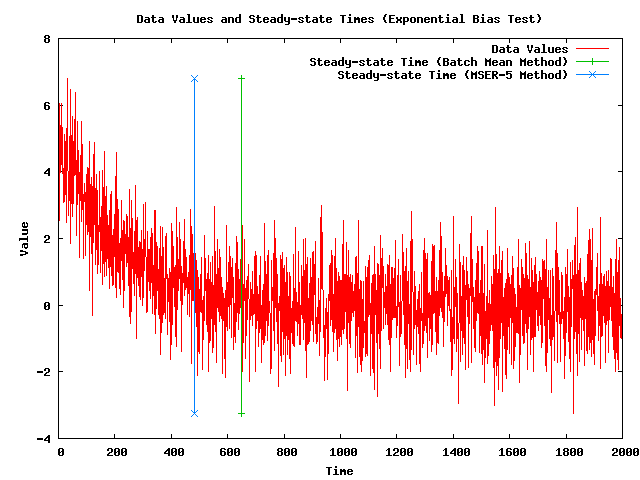
- Note: The BM method is giving a steady-state time after steady-state has been reached, which would cause it to delete more values than the MSER-5 method.
- Note: The following plot shows the steady-state times calculated as a function of the number of data values for the simulated data set with an exponential bias.
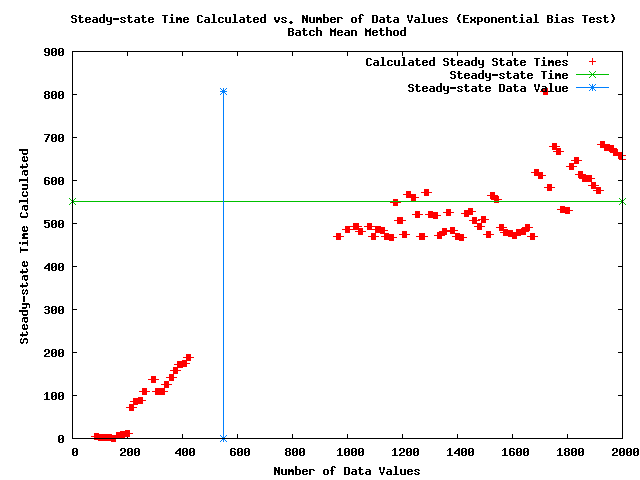
- Note: The above figure shows a problem with the BM method that data sets with fewer values than are required for steady-state (to the left of the blue line) are being called steady-state by the algorithm and giving steady-state times much less than the true steady-state time (the green line).
- Note: The following plot shows a simulated data set (with 2,000 data values) that has a linearly increasing bias. My implementation of the Batch Mean (BM) algorithm did not find a steady-state time for this number of data values.
- Note: The following plot shows the steady-state times calculated as a function of the number of data values for the simulated data set with a linearly increasing bias.
- Note: The above figure shows a problem with the BM method that data sets that are not at steady-state, i.e. all of the data values in this data set, are being called steady-state by the algorithm.
- Note: Because the Batch Mean (BM) algorithm is detecting steady-state for data sets that are not in steady-state, it is being REJECTED.


MANET Routing ExampLe Data
- Note: There are now 2 steady-state detectors in the SAFE MANET example:
- Packets Received
- Receive Rate
- Note: Although the plots have different numerical values for packets-received and receive-rate, they do have the same shape, which means the 2 quantities appear to be linearly related.
- Note: I made the example run for 1000 seconds so that it would be in steady-state.
- Note: The attached plots make it look like the MSER-5 method works well for simulations like this that have achieved steady-state.
- Note: The following 2 plots show 1000 and 200 seconds from the MANET packets-received data set along with the steady-state times that my implementations of the Batch Mean (BM) algorithm and the MSER-5 algrothm are currently returning. The plots also show vertical lines where the steady-state times are.
- Note: The BM method is giving a steady-state time before steady-state has been reached, which would cause it to include unwanted values that the MSER-5 method does not.
- Note: The following plot shows the steady-state times calculated as a function of the number of data values for the MANET packets-received data set.
- Note: The above figure shows a problem with the BM method that data sets with fewer values than are required for steady-state for times up to around 120 seconds are being called steady-state by the algorithm and giving steady-state times much less than the true steady-state time, which is around 60 seconds.
- Note: The following 2 plots show 1000 and 200 seconds from the MANET receive-rate data set along with the steady-state times that my implementations of the Batch Mean (BM) algorithm and the MSER-5 algrothm are currently returning. The plots also show vertical lines where the steady-state times are.
- Note: The BM method is giving a steady-state time before steady-state has been reached, which would cause it to include unwanted values that the MSER-5 method does not.
- Note: The following plot shows the steady-state times calculated as a function of the number of data values for the MANET receive-rate data set.
- Note: The above figure shows a problem with the BM method that data sets with fewer values than are required for steady-state for times up to around 120 seconds are being called steady-state by the algorithm and giving steady-state times much less than the true steady-state time, which is around 60 seconds.
- Note: Because the Batch Mean (BM) algorithm is detecting steady-state for data sets that are not in steady-state, it is being REJECTED.


Conclusion
A more robust steady-state detection algorithm than the Batch Mean (BM) algorithm should be implemented that will then be coupled with the MSER-5 method that appears to work well for simulations once they have achieved steady-state.
Algorithms to Try (In order that they should be tried)
- Schruben's Maximum Test
- Schruben, L. (1982). Detecting Initialisation Bias in Simulation Output. Operations Research, 30(3), 569-590.
- Summary: Standardized time series methods for steady-state detection.
- Advantages: Single-replicate algorithm.
- Disadvantages:
- Note:
- Schruben's Optimal Test
- Schruben, L., Singh, H., and Tierney, L. (1983). Optimal Tests for Initialisation Bias in Simulation Output. Operations Research, 31( 6), 1167-1178.
- Summary: Standardized time series methods for steady-state detection.
- Advantages: Single-replicate algorithm.
- Disadvantages:
- Note:
- Batch means
- Law, A. M. (2007). Simulation Modeling and Analysis. 4th ed. New York: McGraw-Hill. (See pp. 528–529.)
- Summary: Groups values into batches and computes mean of each batch.
- Advantages:
- Disadvantages:
- Note: