Welcome to ns-3’s manual!
This is the ns-3 manual. Primary documentation for the ns-3 project is available in four forms:
- ns-3 Doxygen: Documentation of the public APIs of the simulator
- Tutorial
- Reference Manual: (this document)
- ns-3 wiki
This document is written in reStructuredText for Sphinx and is maintained in the doc/manual directory of ns-3’s source code.
Organization
This chapter describes the overall ns-3 software organization and the corresponding organization of this manual.
ns-3 is a discrete-event network simulator in which the simulation core and models are implemented in C++. ns-3 is built as a library which may be statically or dynamically linked to a C++ main program that defines the simulation topology and starts the simulator. ns-3 also exports nearly all of its API to Python, allowing Python programs to import an “ns3” module in much the same way as the ns-3 library is linked by executables in C++.
Software organization of ns-3
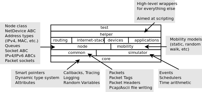
The source code for ns-3 is mostly organized in the src directory and can be described by the diagram in Software organization of ns-3. We will work our way from the bottom up; in general, modules only have dependencies on modules beneath them in the figure.
We first describe the core of the simulator; those components that are common across all protocol, hardware, and environmental models. The simulation core is implemented in src/core, and the core is used to build the simulation engine src/simulator. Packets are fundamental objects in a network simulator and are implemented in src/common. These three simulation modules by themselves are intended to comprise a generic simulation core that can be used by different kinds of networks, not just Internet-based networks. The above modules of ns-3 are independent of specific network and device models, which are covered in subsequent parts of this manual.
In addition to the above ns-3 core, we introduce, also in the initial portion of the manual, two other modules that supplement the core C++-based API. ns-3 programs may access all of the API directly or may make use of a so-called helper API that provides convenient wrappers or encapsulation of low-level API calls. The fact that ns-3 programs can be written to two APIs (or a combination thereof) is a fundamental aspect of the simulator. We also describe how Python is supported in ns-3 before moving onto specific models of relevance to network simulation.
The remainder of the manual is focused on documenting the models and supporting capabilities. The next part focuses on two fundamental objects in ns-3: the Node and NetDevice. Two special NetDevice types are designed to support network emulation use cases, and emulation is described next. The following chapter is devoted to Internet-related models, including the sockets API used by Internet applications. The next chapter covers applications, and the following chapter describes additional support for simulation, such as animators and statistics.
The project maintains a separate manual devoted to testing and validation of ns-3 code (see the ns-3 Testing and Validation manual).
Core
Random Variables
ns-3 contains a built-in pseudo-random number generator (PRNG). It is important for serious users of the simulator to understand the functionality, configuration, and usage of this PRNG, and to decide whether it is sufficient for his or her research use.
Quick Overview
ns-3 random numbers are provided via instances of ns3::RandomVariable.
- by default, ns-3 simulations use a fixed seed; if there is any randomness in the simulation, each run of the program will yield identical results unless the seed and/or run number is changed.
- in ns-3.3 and earlier, ns-3 simulations used a random seed by default; this marks a change in policy starting with ns-3.4.
- to obtain randomness across multiple simulation runs, you must either set the seed differently or set the run number differently. To set a seed, call ns3::SeedManager::SetSeed() at the beginning of the program; to set a run number with the same seed, call ns3::SeedManager::SetRun() at the beginning of the program; see Seeding and independent replications.
- each RandomVariable used in ns-3 has a virtual random number generator associated with it; all random variables use either a fixed or random seed based on the use of the global seed (previous bullet);
- if you intend to perform multiple runs of the same scenario, with different random numbers, please be sure to read the section on how to perform independent replications: Seeding and independent replications.
Read further for more explanation about the random number facility for ns-3.
Background
Simulations use a lot of random numbers; one study found that most network simulations spend as much as 50% of the CPU generating random numbers. Simulation users need to be concerned with the quality of the (pseudo) random numbers and the independence between different streams of random numbers.
Users need to be concerned with a few issues, such as:
- the seeding of the random number generator and whether a simulation outcome is deterministic or not,
- how to acquire different streams of random numbers that are independent from one another, and
- how long it takes for streams to cycle
We will introduce a few terms here: a RNG provides a long sequence of (pseudo) random numbers. The length of this sequence is called the cycle length or period, after which the RNG will repeat itself. This sequence can be partitioned into disjoint streams. A stream of a RNG is a contiguous subset or block of the RNG sequence. For instance, if the RNG period is of length N, and two streams are provided from this RNG, then the first stream might use the first N/2 values and the second stream might produce the second N/2 values. An important property here is that the two streams are uncorrelated. Likewise, each stream can be partitioned disjointedly to a number of uncorrelated substreams. The underlying RNG hopefully produces a pseudo-random sequence of numbers with a very long cycle length, and partitions this into streams and substreams in an efficient manner.
ns-3 uses the same underlying random number generator as does ns-2: the
MRG32k3a generator from Pierre L’Ecuyer. A detailed description can be found in
http://www.iro.umontreal.ca/~lecuyer/myftp/papers/streams00.pdf. The MRG32k3a
generator provides  independent streams of random numbers,
each of which consists of
independent streams of random numbers,
each of which consists of  substreams. Each substream has a
period (i.e., the number of random numbers before overlap) of
substreams. Each substream has a
period (i.e., the number of random numbers before overlap) of
 . The period of the entire generator is
  .
.
Class ns3::RandomVariable is the public interface to this underlying random number generator. When users create new RandomVariables (such as ns3::UniformVariable, ns3::ExponentialVariable, etc.), they create an object that uses one of the distinct, independent streams of the random number generator. Therefore, each object of type ns3::RandomVariable has, conceptually, its own “virtual” RNG. Furthermore, each ns3::RandomVariable can be configured to use one of the set of substreams drawn from the main stream.
An alternate implementation would be to allow each RandomVariable to have its own (differently seeded) RNG. However, we cannot guarantee as strongly that the different sequences would be uncorrelated in such a case; hence, we prefer to use a single RNG and streams and substreams from it.
Seeding and independent replications
ns-3 simulations can be configured to produce deterministic or random results. If the ns-3 simulation is configured to use a fixed, deterministic seed with the same run number, it should give the same output each time it is run.
By default, ns-3 simulations use a fixed seed and run number. These values are stored in two ns3::GlobalValue instances: g_rngSeed and g_rngRun.
A typical use case is to run a simulation as a sequence of independent trials, so as to compute statistics on a large number of independent runs. The user can either change the global seed and rerun the simulation, or can advance the substream state of the RNG, which is referred to as incrementing the run number.
A class ns3::SeedManager provides an API to control the seeding and run number behavior. This seeding and substream state setting must be called before any random variables are created; e.g:
SeedManager::SetSeed (3);  // Changes seed from default of 1 to 3
SeedManager::SetRun (7);  // Changes run number from default of 1 to 7
// Now, create random variables
UniformVariable x(0,10);
ExponentialVariable y(2902);
...
Which is better, setting a new seed or advancing the substream state? There is
no guarantee that the streams produced by two random seeds will not overlap.
The only way to guarantee that two streams do not overlap is to use the
substream capability provided by the RNG implementation. Therefore, use the
substream capability to produce multiple independent runs of the same
simulation. In other words, the more statistically rigorous way to configure
multiple independent replications is to use a fixed seed and to advance the run
number. This implementation allows for a maximum of
independent replications using the substreams.
For ease of use, it is not necessary to control the seed and run number from within the program; the user can set the NS_GLOBAL_VALUE environment variable as follows:
NS_GLOBAL_VALUE="RngRun=3" ./waf --run program-name
Another way to control this is by passing a command-line argument; since this is an ns-3 GlobalValue instance, it is equivalently done such as follows:
./waf --command-template="%s --RngRun=3" --run program-name
or, if you are running programs directly outside of waf:
./build/optimized/scratch/program-name --RngRun=3
The above command-line variants make it easy to run lots of different runs from a shell script by just passing a different RngRun index.
Class RandomVariable
All random variables should derive from class RandomVariable. This base class provides a few static methods for globally configuring the behavior of the random number generator. Derived classes provide API for drawing random variates from the particular distribution being supported.
Each RandomVariable created in the simulation is given a generator that is a new
RNGStream from the underlying PRNG. Used in this manner, the L’Ecuyer
implementation allows for a maximum of  random variables. Each
random variable in a single replication can produce up to
random variables. Each
random variable in a single replication can produce up to  random numbers before overlapping.
Base class public API
Below are excerpted a few public methods of class RandomVariable that access the next value in the substream.:
/**
 * \brief Returns a random double from the underlying distribution
 * \return A floating point random value
 */
double GetValue (void) const;

/**
 * \brief Returns a random integer integer from the underlying distribution
 * \return  Integer cast of ::GetValue()
 */
uint32_t GetInteger (void) const;
We have already described the seeding configuration above. Different RandomVariable subclasses may have additional API.
Types of RandomVariables
The following types of random variables are provided, and are documented in the ns-3 Doxygen or by reading src/core/random-variable.h. Users can also create their own custom random variables by deriving from class RandomVariable.
- class UniformVariable
- class ConstantVariable
- class SequentialVariable
- class ExponentialVariable
- class ParetoVariable
- class WeibullVariable
- class NormalVariable
- class EmpiricalVariable
- class IntEmpiricalVariable
- class DeterministicVariable
- class LogNormalVariable
- class TriangularVariable
- class GammaVariable
- class ErlangVariable
- class ZipfVariable
Semantics of RandomVariable objects
RandomVariable objects have value semantics. This means that they can be passed by value to functions. The can also be passed by reference to const. RandomVariables do not derive from ns3::Object and we do not use smart pointers to manage them; they are either allocated on the stack or else users explicitly manage any heap-allocated RandomVariables.
RandomVariable objects can also be used in ns-3 attributes, which means that values can be set for them through the ns-3 attribute system. An example is in the propagation models for WifiNetDevice::
TypeId
RandomPropagationDelayModel::GetTypeId (void)
{
  static TypeId tid = TypeId ("ns3::RandomPropagationDelayModel")
    .SetParent<PropagationDelayModel> ()
    .AddConstructor<RandomPropagationDelayModel> ()
    .AddAttribute ("Variable",
                   "The random variable which generates random delays (s).",
                   RandomVariableValue (UniformVariable (0.0, 1.0)),
         MakeRandomVariableAccessor (&RandomPropagationDelayModel::m_variable),
                   MakeRandomVariableChecker ())
    ;
  return tid;
}
Here, the ns-3 user can change the default random variable for this delay model (which is a UniformVariable ranging from 0 to 1) through the attribute system.
Using other PRNG
There is presently no support for substituting a different underlying random number generator (e.g., the GNU Scientific Library or the Akaroa package). Patches are welcome.
More advanced usage
To be completed.
Publishing your results
When you publish simulation results, a key piece of configuration information that you should always state is how you used the the random number generator.
- what seeds you used,
- what RNG you used if not the default,
- how were independent runs performed,
- for large simulations, how did you check that you did not cycle.
It is incumbent on the researcher publishing results to include enough information to allow others to reproduce his or her results. It is also incumbent on the researcher to convince oneself that the random numbers used were statistically valid, and to state in the paper why such confidence is assumed.
Summary
Let’s review what things you should do when creating a simulation.
- Decide whether you are running with a fixed seed or random seed; a fixed seed is the default,
- Decide how you are going to manage independent replications, if applicable,
- Convince yourself that you are not drawing more random values than the cycle length, if you are running a very long simulation, and
- When you publish, follow the guidelines above about documenting your use of the random number generator.
Callbacks
Some new users to ns-3 are unfamiliar with an extensively used programming idiom used throughout the code: the ns-3 callback. This chapter provides some motivation on the callback, guidance on how to use it, and details on its implementation.
Callbacks Motivation
Consider that you have two simulation models A and B, and you wish to have them pass information between them during the simulation. One way that you can do that is that you can make A and B each explicitly knowledgeable about the other, so that they can invoke methods on each other:
class A {
public:
  void ReceiveInput ( // parameters );
  ...
}

(in another source file:)

class B {
public:
  void DoSomething (void);
  ...

private:
  A* a_instance; // pointer to an A
}

void
B::DoSomething()
{
  // Tell a_instance that something happened
  a_instance->ReceiveInput ( // parameters);
  ...
}
This certainly works, but it has the drawback that it introduces a dependency on A and B to know about the other at compile time (this makes it harder to have independent compilation units in the simulator) and is not generalized; if in a later usage scenario, B needs to talk to a completely different C object, the source code for B needs to be changed to add a c_instance and so forth. It is easy to see that this is a brute force mechanism of communication that can lead to programming cruft in the models.
This is not to say that objects should not know about one another if there is a hard dependency between them, but that often the model can be made more flexible if its interactions are less constrained at compile time.
This is not an abstract problem for network simulation research, but rather it has been a source of problems in previous simulators, when researchers want to extend or modify the system to do different things (as they are apt to do in research). Consider, for example, a user who wants to add an IPsec security protocol sublayer between TCP and IP:
------------                   -----------
|   TCP    |                   |  TCP    |
------------                   -----------
     |           becomes ->        |
-----------                    -----------
|   IP    |                    | IPsec   |
-----------                    -----------
                                   |
                               -----------
                               |   IP    |
                               -----------
If the simulator has made assumptions, and hard coded into the code, that IP always talks to a transport protocol above, the user may be forced to hack the system to get the desired interconnections. This is clearly not an optimal way to design a generic simulator.
Callbacks Background
Note
Readers familiar with programming callbacks may skip this tutorial section.
The basic mechanism that allows one to address the problem above is known as a callback. The ultimate goal is to allow one piece of code to call a function (or method in C++) without any specific inter-module dependency.
This ultimately means you need some kind of indirection – you treat the address of the called function as a variable. This variable is called a pointer-to-function variable. The relationship between function and pointer-to-function pointer is really no different that that of object and pointer-to-object.
In C the canonical example of a pointer-to-function is a pointer-to-function-returning-integer (PFI). For a PFI taking one int parameter, this could be declared like,:
int (*pfi)(int arg) = 0;
What you get from this is a variable named simply pfi that is initialized to the value 0. If you want to initialize this pointer to something meaningful, you have to have a function with a matching signature. In this case:
int MyFunction (int arg) {}
If you have this target, you can initialize the variable to point to your function like:
pfi = MyFunction;
You can then call MyFunction indirectly using the more suggestive form of the call:
int result = (*pfi) (1234);
This is suggestive since it looks like you are dereferencing the function pointer just like you would dereference any pointer. Typically, however, people take advantage of the fact that the compiler knows what is going on and will just use a shorter form:
int result = pfi (1234);
Notice that the function pointer obeys value semantics, so you can pass it around like any other value. Typically, when you use an asynchronous interface you will pass some entity like this to a function which will perform an action and call back to let you know it completed. It calls back by following the indirection and executing the provided function.
In C++ you have the added complexity of objects. The analogy with the PFI above means you have a pointer to a member function returning an int (PMI) instead of the pointer to function returning an int (PFI).
The declaration of the variable providing the indirection looks only slightly different:
int (MyClass::*pmi) (int arg) = 0;
This declares a variable named pmi just as the previous example declared a variable named pfi. Since the will be to call a method of an instance of a particular class, one must declare that method in a class:
class MyClass {
public:
  int MyMethod (int arg);
};
Given this class declaration, one would then initialize that variable like this:
pmi = &MyClass::MyMethod;
This assigns the address of the code implementing the method to the variable, completing the indirection. In order to call a method, the code needs a this pointer. This, in turn, means there must be an object of MyClass to refer to. A simplistic example of this is just calling a method indirectly (think virtual function):
int (MyClass::*pmi) (int arg) = 0;  // Declare a PMI
pmi = &MyClass::MyMethod;           // Point at the implementation code

MyClass myClass;                    // Need an instance of the class
(myClass.*pmi) (1234);              // Call the method with an object ptr
Just like in the C example, you can use this in an asynchronous call to another module which will call back using a method and an object pointer. The straightforward extension one might consider is to pass a pointer to the object and the PMI variable. The module would just do:
(*objectPtr.*pmi) (1234);
to execute the callback on the desired object.
One might ask at this time, what’s the point? The called module will have to understand the concrete type of the calling object in order to properly make the callback. Why not just accept this, pass the correctly typed object pointer and do object->Method(1234) in the code instead of the callback? This is precisely the problem described above. What is needed is a way to decouple the calling function from the called class completely. This requirement led to the development of the Functor.
A functor is the outgrowth of something invented in the 1960s called a closure. It is basically just a packaged-up function call, possibly with some state.
A functor has two parts, a specific part and a generic part, related through inheritance. The calling code (the code that executes the callback) will execute a generic overloaded operator () of a generic functor to cause the callback to be called. The called code (the code that wants to be called back) will have to provide a specialized implementation of the operator () that performs the class-specific work that caused the close-coupling problem above.
With the specific functor and its overloaded operator () created, the called code then gives the specialized code to the module that will execute the callback (the calling code).
The calling code will take a generic functor as a parameter, so an implicit cast is done in the function call to convert the specific functor to a generic functor. This means that the calling module just needs to understand the generic functor type. It is decoupled from the calling code completely.
The information one needs to make a specific functor is the object pointer and the pointer-to-method address.
The essence of what needs to happen is that the system declares a generic part of the functor:
template <typename T>
class Functor
{
public:
    virtual void operator() (T arg) = 0;
 };
The caller defines a specific part of the functor that really is just there to implement the specific operator() method:
template <typename T, typename ARG>
class SpecificFunctor : public Functor
 {
 public:
    SpecificFunctor(T* p, int (T::*_pmi)(ARG arg))
    {
      m_p = p;
      m_pmi = pmi;
    }

    virtual int operator() (ARG arg)
    {
      (*m_p.*m_pmi)(arg);
    }
private:
    void (T::*m_pmi)(ARG arg);
    T* m_p;
 };
Object model
ns-3 is fundamentally a C++ object system. Objects can be declared and instantiated as usual, per C++ rules. ns-3 also adds some features to traditional C++ objects, as described below, to provide greater functionality and features. This manual chapter is intended to introduce the reader to the ns-3 object model.
This section describes the C++ class design for ns-3 objects. In brief, several design patterns in use include classic object-oriented design (polymorphic interfaces and implementations), separation of interface and implementation, the non-virtual public interface design pattern, an object aggregation facility, and reference counting for memory management. Those familiar with component models such as COM or Bonobo will recognize elements of the design in the ns-3 object aggregation model, although the ns-3 design is not strictly in accordance with either.
Object-oriented behavior
C++ objects, in general, provide common object-oriented capabilities (abstraction, encapsulation, inheritance, and polymorphism) that are part of classic object-oriented design. ns-3 objects make use of these properties; for instance::
class Address
{
public:
  Address ();
  Address (uint8_t type, const uint8_t *buffer, uint8_t len);
  Address (const Address & address);
  Address &operator = (const Address &address);
  ...
private:
  uint8_t m_type;
  uint8_t m_len;
  ...
};
Object base classes
There are three special base classes used in ns-3. Classes that inherit from these base classes can instantiate objects with special properties. These base classes are:
- class Object
- class ObjectBase
- class SimpleRefCount
It is not required that ns-3 objects inherit from these class, but those that do get special properties. Classes deriving from class Object get the following properties.
- the ns-3 type and attribute system (see Attributes)
- an object aggregation system
- a smart-pointer reference counting system (class Ptr)
Classes that derive from class ObjectBase get the first two properties above, but do not get smart pointers. Classes that derive from class SimpleRefCount: get only the smart-pointer reference counting system.
In practice, class Object is the variant of the three above that the ns-3 developer will most commonly encounter.
Memory management and class Ptr
Memory management in a C++ program is a complex process, and is often done incorrectly or inconsistently. We have settled on a reference counting design described as follows.
All objects using reference counting maintain an internal reference count to determine when an object can safely delete itself. Each time that a pointer is obtained to an interface, the object’s reference count is incremented by calling Ref(). It is the obligation of the user of the pointer to explicitly Unref() the pointer when done. When the reference count falls to zero, the object is deleted.
- When the client code obtains a pointer from the object itself through object creation, or via GetObject, it does not have to increment the reference count.
- When client code obtains a pointer from another source (e.g., copying a pointer) it must call Ref() to increment the reference count.
- All users of the object pointer must call Unref() to release the reference.
The burden for calling Unref() is somewhat relieved by the use of the reference counting smart pointer class described below.
Users using a low-level API who wish to explicitly allocate non-reference-counted objects on the heap, using operator new, are responsible for deleting such objects.
Reference counting smart pointer (Ptr)
Calling Ref() and Unref() all the time would be cumbersome, so ns-3 provides a smart pointer class Ptr similar to Boost::intrusive_ptr. This smart-pointer class assumes that the underlying type provides a pair of Ref and Unref methods that are expected to increment and decrement the internal refcount of the object instance.
This implementation allows you to manipulate the smart pointer as if it was a normal pointer: you can compare it with zero, compare it against other pointers, assign zero to it, etc.
It is possible to extract the raw pointer from this smart pointer with the GetPointer() and PeekPointer() methods.
If you want to store a newed object into a smart pointer, we recommend you to use the CreateObject template functions to create the object and store it in a smart pointer to avoid memory leaks. These functions are really small convenience functions and their goal is just to save you a small bit of typing.
CreateObject and Create
Objects in C++ may be statically, dynamically, or automatically created. This holds true for ns-3 also, but some objects in the system have some additional frameworks available. Specifically, reference counted objects are usually allocated using a templated Create or CreateObject method, as follows.
For objects deriving from class Object::
Ptr<WifiNetDevice> device = CreateObject<WifiNetDevice> ();
Please do not create such objects using operator new; create them using CreateObject() instead.
For objects deriving from class SimpleRefCount, or other objects that support usage of the smart pointer class, a templated helper function is available and recommended to be used::
Ptr<B> b = Create<B> ();
This is simply a wrapper around operator new that correctly handles the reference counting system.
In summary, use Create<B> if B is not an object but just uses reference counting (e.g. Packet), and use CreateObject<B> if B derives from ns3::Object.
Aggregation
The ns-3 object aggregation system is motivated in strong part by a recognition that a common use case for ns-2 has been the use of inheritance and polymorphism to extend protocol models. For instance, specialized versions of TCP such as RenoTcpAgent derive from (and override functions from) class TcpAgent.
However, two problems that have arisen in the ns-2 model are downcasts and “weak base class.” Downcasting refers to the procedure of using a base class pointer to an object and querying it at run time to find out type information, used to explicitly cast the pointer to a subclass pointer so that the subclass API can be used. Weak base class refers to the problems that arise when a class cannot be effectively reused (derived from) because it lacks necessary functionality, leading the developer to have to modify the base class and causing proliferation of base class API calls, some of which may not be semantically correct for all subclasses.
ns-3 is using a version of the query interface design pattern to avoid these problems. This design is based on elements of the Component Object Model and GNOME Bonobo although full binary-level compatibility of replaceable components is not supported and we have tried to simplify the syntax and impact on model developers.
Aggregation example
Node is a good example of the use of aggregation in ns-3. Note that there are not derived classes of Nodes in ns-3 such as class InternetNode. Instead, components (protocols) are aggregated to a node. Let’s look at how some Ipv4 protocols are added to a node.:
static void
AddIpv4Stack(Ptr<Node> node)
{
  Ptr<Ipv4L3Protocol> ipv4 = CreateObject<Ipv4L3Protocol> ();
  ipv4->SetNode (node);
  node->AggregateObject (ipv4);
  Ptr<Ipv4Impl> ipv4Impl = CreateObject<Ipv4Impl> ();
  ipv4Impl->SetIpv4 (ipv4);
  node->AggregateObject (ipv4Impl);
}
Note that the Ipv4 protocols are created using CreateObject(). Then, they are aggregated to the node. In this manner, the Node base class does not need to be edited to allow users with a base class Node pointer to access the Ipv4 interface; users may ask the node for a pointer to its Ipv4 interface at runtime. How the user asks the node is described in the next subsection.
Note that it is a programming error to aggregate more than one object of the same type to an ns3::Object. So, for instance, aggregation is not an option for storing all of the active sockets of a node.
GetObject example
GetObject is a type-safe way to achieve a safe downcasting and to allow interfaces to be found on an object.
Consider a node pointer m_node that points to a Node object that has an implementation of IPv4 previously aggregated to it. The client code wishes to configure a default route. To do so, it must access an object within the node that has an interface to the IP forwarding configuration. It performs the following::
Ptr<Ipv4> ipv4 = m_node->GetObject<Ipv4> ();
If the node in fact does not have an Ipv4 object aggregated to it, then the method will return null. Therefore, it is good practice to check the return value from such a function call. If successful, the user can now use the Ptr to the Ipv4 object that was previously aggregated to the node.
Another example of how one might use aggregation is to add optional models to objects. For instance, an existing Node object may have an “Energy Model” object aggregated to it at run time (without modifying and recompiling the node class). An existing model (such as a wireless net device) can then later “GetObject” for the energy model and act appropriately if the interface has been either built in to the underlying Node object or aggregated to it at run time. However, other nodes need not know anything about energy models.
We hope that this mode of programming will require much less need for developers to modify the base classes.
Object factories
A common use case is to create lots of similarly configured objects. One can repeatedly call CreateObject() but there is also a factory design pattern in use in the ns-3 system. It is heavily used in the “helper” API.
Class ObjectFactory can be used to instantiate objects and to configure the attributes on those objects:
void SetTypeId (TypeId tid);
void Set (std::string name, const AttributeValue &value);
Ptr<T> Create (void) const;
The first method allows one to use the ns-3 TypeId system to specify the type of objects created. The second allows one to set attributes on the objects to be created, and the third allows one to create the objects themselves.
For example:
ObjectFactory factory;
// Make this factory create objects of type FriisPropagationLossModel
factory.SetTypeId ("ns3::FriisPropagationLossModel")
// Make this factory object change a default value of an attribute, for
// subsequently created objects
factory.Set ("SystemLoss", DoubleValue (2.0));
// Create one such object
Ptr<Object> object = m_factory.Create ();
factory.Set ("SystemLoss", DoubleValue (3.0));
// Create another object
Ptr<Object> object = m_factory.Create ();
Downcasting
A question that has arisen several times is, “If I have a base class pointer (Ptr) to an object and I want the derived class pointer, should I downcast (via C++ dynamic cast) to get the derived pointer, or should I use the object aggregation system to GetObject<> () to find a Ptr to the interface to the subclass API?”
The answer to this is that in many situations, both techniques will work. ns-3 provides a templated function for making the syntax of Object dynamic casting much more user friendly::
template <typename T1, typename T2>
Ptr<T1>
DynamicCast (Ptr<T2> const&p)
{
  return Ptr<T1> (dynamic_cast<T1 *> (PeekPointer (p)));
}
DynamicCast works when the programmer has a base type pointer and is testing against a subclass pointer. GetObject works when looking for different objects aggregated, but also works with subclasses, in the same way as DynamicCast. If unsure, the programmer should use GetObject, as it works in all cases. If the programmer knows the class hierarchy of the object under consideration, it is more direct to just use DynamicCast.
Attributes
In ns-3 simulations, there are two main aspects to configuration:
- the simulation topology and how objects are connected
- the values used by the models instantiated in the topology
This chapter focuses on the second item above: how the many values in use in ns-3 are organized, documented, and modifiable by ns-3 users. The ns-3 attribute system is also the underpinning of how traces and statistics are gathered in the simulator.
Before delving into details of the attribute value system, it will help to review some basic properties of class ns3::Object.
Object Overview
ns-3 is fundamentally a C++ object-based system. By this we mean that new C++ classes (types) can be declared, defined, and subclassed as usual.
Many ns-3 objects inherit from the ns3::Object base class. These objects have some additional properties that we exploit for organizing the system and improving the memory management of our objects:
- a “metadata” system that links the class name to a lot of meta-information about the object, including the base class of the subclass, the set of accessible constructors in the subclass, and the set of “attributes” of the subclass
- a reference counting smart pointer implementation, for memory management.
ns-3 objects that use the attribute system derive from either ns3::Object or ns3::ObjectBase. Most ns-3 objects we will discuss derive from ns3::Object, but a few that are outside the smart pointer memory management framework derive from ns3::ObjectBase.
Let’s review a couple of properties of these objects.
Smart pointers
As introduced in the ns-3 tutorial, ns-3 objects are memory managed by a reference counting smart pointer implementation, class ns3::Ptr.
Smart pointers are used extensively in the ns-3 APIs, to avoid passing references to heap-allocated objects that may cause memory leaks. For most basic usage (syntax), treat a smart pointer like a regular pointer::
Ptr<WifiNetDevice> nd = ...;
nd->CallSomeFunction ();
// etc.
CreateObject
As we discussed above in Memory management and class Ptr, at the lowest-level API, objects of type ns3::Object are not instantiated using operator new as usual but instead by a templated function called CreateObject().
A typical way to create such an object is as follows::
Ptr<WifiNetDevice> nd = CreateObject<WifiNetDevice> ();
You can think of this as being functionally equivalent to::
WifiNetDevice* nd = new WifiNetDevice ();
Objects that derive from ns3::Object must be allocated on the heap using CreateObject(). Those deriving from ns3::ObjectBase, such as ns-3 helper functions and packet headers and trailers, can be allocated on the stack.
In some scripts, you may not see a lot of CreateObject() calls in the code; this is because there are some helper objects in effect that are doing the CreateObject()s for you.
TypeId
ns-3 classes that derive from class ns3::Object can include a metadata class called TypeId that records meta-information about the class, for use in the object aggregation and component manager systems:
- a unique string identifying the class
- the base class of the subclass, within the metadata system
- the set of accessible constructors in the subclass
Object Summary
Putting all of these concepts together, let’s look at a specific example: class ns3::Node.
The public header file node.h has a declaration that includes a static GetTypeId function call::
class Node : public Object
{
public:
  static TypeId GetTypeId (void);
  ...
This is defined in the node.cc file as follows::
TypeId
Node::GetTypeId (void)
{
  static TypeId tid = TypeId ("ns3::Node")
    .SetParent<Object> ()
    .AddConstructor<Node> ()
    .AddAttribute ("DeviceList", "The list of devices associated to this Node.",
                   ObjectVectorValue (),
                   MakeObjectVectorAccessor (&Node::m_devices),
                   MakeObjectVectorChecker<NetDevice> ())
    .AddAttribute ("ApplicationList", "The list of applications associated to this Node.",
                   ObjectVectorValue (),
                   MakeObjectVectorAccessor (&Node::m_applications),
                   MakeObjectVectorChecker<Application> ())
    .AddAttribute ("Id", "The id (unique integer) of this Node.",
                   TypeId::ATTR_GET, // allow only getting it.
                   UintegerValue (0),
                   MakeUintegerAccessor (&Node::m_id),
                   MakeUintegerChecker<uint32_t> ())
    ;
  return tid;
}
Consider the TypeId of an ns-3 Object class as an extended form of run time type information (RTTI). The C++ language includes a simple kind of RTTI in order to support dynamic_cast and typeid operators.
The “.SetParent<Object> ()” call in the declaration above is used in conjunction with our object aggregation mechanisms to allow safe up- and down-casting in inheritance trees during GetObject.
The “.AddConstructor<Node> ()” call is used in conjunction with our abstract object factory mechanisms to allow us to construct C++ objects without forcing a user to know the concrete class of the object she is building.
The three calls to “.AddAttribute” associate a given string with a strongly typed value in the class. Notice that you must provide a help string which may be displayed, for example, via command line processors. Each Attribute is associated with mechanisms for accessing the underlying member variable in the object (for example, MakeUintegerAccessor tells the generic Attribute code how to get to the node ID above). There are also “Checker” methods which are used to validate values.
When users want to create Nodes, they will usually call some form of CreateObject,:
Ptr<Node> n = CreateObject<Node> ();
or more abstractly, using an object factory, you can create a Node object without even knowing the concrete C++ type:
ObjectFactory factory;
const std::string typeId = "ns3::Node'';
factory.SetTypeId (typeId);
Ptr<Object> node = factory.Create <Object> ();
Both of these methods result in fully initialized attributes being available in the resulting Object instances.
We next discuss how attributes (values associated with member variables or functions of the class) are plumbed into the above TypeId.
Attribute Overview
The goal of the attribute system is to organize the access of internal member objects of a simulation. This goal arises because, typically in simulation, users will cut and paste/modify existing simulation scripts, or will use higher-level simulation constructs, but often will be interested in studying or tracing particular internal variables. For instance, use cases such as:
- “I want to trace the packets on the wireless interface only on the first access point”
- “I want to trace the value of the TCP congestion window (every time it changes) on a particular TCP socket”
- “I want a dump of all values that were used in my simulation.”
Similarly, users may want fine-grained access to internal variables in the simulation, or may want to broadly change the initial value used for a particular parameter in all subsequently created objects. Finally, users may wish to know what variables are settable and retrievable in a simulation configuration. This is not just for direct simulation interaction on the command line; consider also a (future) graphical user interface that would like to be able to provide a feature whereby a user might right-click on an node on the canvas and see a hierarchical, organized list of parameters that are settable on the node and its constituent member objects, and help text and default values for each parameter.
Functional overview
We provide a way for users to access values deep in the system, without having to plumb accessors (pointers) through the system and walk pointer chains to get to them. Consider a class DropTailQueue that has a member variable that is an unsigned integer m_maxPackets; this member variable controls the depth of the queue.
If we look at the declaration of DropTailQueue, we see the following::
class DropTailQueue : public Queue {
public:
  static TypeId GetTypeId (void);
  ...

private:
  std::queue<Ptr<Packet> > m_packets;
  uint32_t m_maxPackets;
};
Let’s consider things that a user may want to do with the value of m_maxPackets:
- Set a default value for the system, such that whenever a new DropTailQueue is created, this member is initialized to that default.
- Set or get the value on an already instantiated queue.
The above things typically require providing Set() and Get() functions, and some type of global default value.
In the ns-3 attribute system, these value definitions and accessor functions are moved into the TypeId class; e.g.::
NS_OBJECT_ENSURE_REGISTERED (DropTailQueue);

TypeId DropTailQueue::GetTypeId (void)
{
  static TypeId tid = TypeId ("ns3::DropTailQueue")
    .SetParent<Queue> ()
    .AddConstructor<DropTailQueue> ()
    .AddAttribute ("MaxPackets",
                   "The maximum number of packets accepted by this DropTailQueue.",
                   UintegerValue (100),
                   MakeUintegerAccessor (&DropTailQueue::m_maxPackets),
                   MakeUintegerChecker<uint32_t> ())
    ;

  return tid;
}
The AddAttribute() method is performing a number of things with this value:
- Binding the variable m_maxPackets to a string “MaxPackets”
- Providing a default value (100 packets)
- Providing some help text defining the value
- Providing a “checker” (not used in this example) that can be used to set bounds on the allowable range of values
The key point is that now the value of this variable and its default value are accessible in the attribute namespace, which is based on strings such as “MaxPackets” and TypeId strings. In the next section, we will provide an example script that shows how users may manipulate these values.
Note that initialization of the attribute relies on the macro NS_OBJECT_ENSURE_REGISTERED (DropTailQueue) being called; if you leave this out of your new class implementation, your attributes will not be initialized correctly.
While we have described how to create attributes, we still haven’t described how to access and manage these values. For instance, there is no globals.h header file where these are stored; attributes are stored with their classes. Questions that naturally arise are how do users easily learn about all of the attributes of their models, and how does a user access these attributes, or document their values as part of the record of their simulation?
Default values and command-line arguments
Let’s look at how a user script might access these values. This is based on the script found at samples/main-attribute-value.cc, with some details stripped out.:
//
// This is a basic example of how to use the attribute system to
// set and get a value in the underlying system; namely, an unsigned
// integer of the maximum number of packets in a queue
//

int
main (int argc, char *argv[])
{

  // By default, the MaxPackets attribute has a value of 100 packets
  // (this default can be observed in the function DropTailQueue::GetTypeId)
  //
  // Here, we set it to 80 packets.  We could use one of two value types:
  // a string-based value or a Uinteger value
  Config::SetDefault ("ns3::DropTailQueue::MaxPackets", StringValue ("80"));
  // The below function call is redundant
  Config::SetDefault ("ns3::DropTailQueue::MaxPackets", UintegerValue (80));

  // Allow the user to override any of the defaults and the above
  // SetDefaults() at run-time, via command-line arguments
  CommandLine cmd;
  cmd.Parse (argc, argv);
The main thing to notice in the above are the two calls to Config::SetDefault. This is how we set the default value for all subsequently instantiated DropTailQueues. We illustrate that two types of Value classes, a StringValue and a UintegerValue class, can be used to assign the value to the attribute named by “ns3::DropTailQueue::MaxPackets”.
Now, we will create a few objects using the low-level API; here, our newly created queues will not have a m_maxPackets initialized to 100 packets but to 80 packets, because of what we did above with default values.:
Ptr<Node> n0 = CreateObject<Node> ();

Ptr<PointToPointNetDevice> net0 = CreateObject<PointToPointNetDevice> ();
n0->AddDevice (net0);

Ptr<Queue> q = CreateObject<DropTailQueue> ();
net0->AddQueue(q);
At this point, we have created a single node (Node 0) and a single PointToPointNetDevice (NetDevice 0) and added a DropTailQueue to it.
Now, we can manipulate the MaxPackets value of the already instantiated DropTailQueue. Here are various ways to do that.
Pointer-based access
We assume that a smart pointer (Ptr) to a relevant network device is in hand; in the current example, it is the net0 pointer.
One way to change the value is to access a pointer to the underlying queue and modify its attribute.
First, we observe that we can get a pointer to the (base class) queue via the PointToPointNetDevice attributes, where it is called TxQueue:
PointerValue tmp;
net0->GetAttribute ("TxQueue", tmp);
Ptr<Object> txQueue = tmp.GetObject ();
Using the GetObject function, we can perform a safe downcast to a DropTailQueue, where MaxPackets is a member:
Ptr<DropTailQueue> dtq = txQueue->GetObject <DropTailQueue> ();
NS_ASSERT (dtq != 0);
Next, we can get the value of an attribute on this queue. We have introduced wrapper “Value” classes for the underlying data types, similar to Java wrappers around these types, since the attribute system stores values and not disparate types. Here, the attribute value is assigned to a UintegerValue, and the Get() method on this value produces the (unwrapped) uint32_t.:
UintegerValue limit;
dtq->GetAttribute ("MaxPackets", limit);
NS_LOG_INFO ("1.  dtq limit: " << limit.Get () << " packets");
Note that the above downcast is not really needed; we could have done the same using the Ptr<Queue> even though the attribute is a member of the subclass:
txQueue->GetAttribute ("MaxPackets", limit);
NS_LOG_INFO ("2.  txQueue limit: " << limit.Get () << " packets");
Now, let’s set it to another value (60 packets):
txQueue->SetAttribute("MaxPackets", UintegerValue (60));
txQueue->GetAttribute ("MaxPackets", limit);
NS_LOG_INFO ("3.  txQueue limit changed: " << limit.Get () << " packets");
Namespace-based access
An alternative way to get at the attribute is to use the configuration namespace. Here, this attribute resides on a known path in this namespace; this approach is useful if one doesn’t have access to the underlying pointers and would like to configure a specific attribute with a single statement.:
Config::Set ("/NodeList/0/DeviceList/0/TxQueue/MaxPackets", UintegerValue (25));
txQueue->GetAttribute ("MaxPackets", limit);
NS_LOG_INFO ("4.  txQueue limit changed through namespace: " <<
    limit.Get () << " packets");
We could have also used wildcards to set this value for all nodes and all net devices (which in this simple example has the same effect as the previous Set()):
Config::Set ("/NodeList/*/DeviceList/*/TxQueue/MaxPackets", UintegerValue (15));
txQueue->GetAttribute ("MaxPackets", limit);
NS_LOG_INFO ("5.  txQueue limit changed through wildcarded namespace: " <<
    limit.Get () << " packets");
Object Name Service-based access
Another way to get at the attribute is to use the object name service facility. Here, this attribute is found using a name string. This approach is useful if one doesn’t have access to the underlying pointers and it is difficult to determine the required concrete configuration namespaced path.:
Names::Add ("server", serverNode);
Names::Add ("server/eth0", serverDevice);

...

Config::Set ("/Names/server/eth0/TxQueue/MaxPackets", UintegerValue (25));
Object names for a fuller treatment of the ns-3 configuration namespace.
Setting through constructors helper classes
Arbitrary combinations of attributes can be set and fetched from the helper and low-level APIs; either from the constructors themselves::
Ptr<Object> p = CreateObject<MyNewObject> ("n1", v1, "n2", v2, ...);
or from the higher-level helper APIs, such as::
mobility.SetPositionAllocator ("GridPositionAllocator",
                               "MinX", DoubleValue (-100.0),
                               "MinY", DoubleValue (-100.0),
                               "DeltaX", DoubleValue (5.0),
                               "DeltaY", DoubleValue (20.0),
                               "GridWidth", UintegerValue (20),
                               "LayoutType", StringValue ("RowFirst"));
Implementation details
Value classes
Readers will note the new FooValue classes which are subclasses of the AttributeValue base class. These can be thought of as an intermediate class that can be used to convert from raw types to the Values that are used by the attribute system. Recall that this database is holding objects of many types with a single generic type. Conversions to this type can either be done using an intermediate class (IntegerValue, DoubleValue for “floating point”) or via strings. Direct implicit conversion of types to Value is not really practical. So in the above, users have a choice of using strings or values::
p->Set ("cwnd", StringValue ("100")); // string-based setter
p->Set ("cwnd", IntegerValue (100)); // integer-based setter
The system provides some macros that help users declare and define new AttributeValue subclasses for new types that they want to introduce into the attribute system:
- ATTRIBUTE_HELPER_HEADER
- ATTRIBUTE_HELPER_CPP
Initialization order
Attributes in the system must not depend on the state of any other Attribute in this system. This is because an ordering of Attribute initialization is not specified, nor enforced, by the system. A specific example of this can be seen in automated configuration programs such as ns3::ConfigStore. Although a given model may arrange it so that Attributes are initialized in a particular order, another automatic configurator may decide independently to change Attributes in, for example, alphabetic order.
Because of this non-specific ordering, no Attribute in the system may have any dependence on any other Attribute. As a corollary, Attribute setters must never fail due to the state of another Attribute. No Attribute setter may change (set) any other Attribute value as a result of changing its value.
This is a very strong restriction and there are cases where Attributes must set consistently to allow correct operation. To this end we do allow for consistency checking when the attribute is used (cf. NS_ASSERT_MSG or NS_ABORT_MSG).
In general, the attribute code to assign values to the underlying class member variables is executed after an object is constructed. But what if you need the values assigned before the constructor body executes, because you need them in the logic of the constructor? There is a way to do this, used for example in the class ns3::ConfigStore: call ObjectBase::ConstructSelf () as follows::
ConfigStore::ConfigStore ()
{
  ObjectBase::ConstructSelf (AttributeList ());
  // continue on with constructor.
}
Extending attributes
The ns-3 system will place a number of internal values under the attribute system, but undoubtedly users will want to extend this to pick up ones we have missed, or to add their own classes to this.
Adding an existing internal variable to the metadata system
Consider this variable in class TcpSocket::
uint32_t m_cWnd; // Congestion window
Suppose that someone working with TCP wanted to get or set the value of that variable using the metadata system. If it were not already provided by ns-3, the user could declare the following addition in the runtime metadata system (to the TypeId declaration for TcpSocket)::
.AddAttribute ("Congestion window",
               "Tcp congestion window (bytes)",
               UintegerValue (1),
               MakeUintegerAccessor (&TcpSocket::m_cWnd),
               MakeUintegerChecker<uint16_t> ())
Now, the user with a pointer to the TcpSocket can perform operations such as setting and getting the value, without having to add these functions explicitly. Furthermore, access controls can be applied, such as allowing the parameter to be read and not written, or bounds checking on the permissible values can be applied.
Adding a new TypeId
Here, we discuss the impact on a user who wants to add a new class to ns-3; what additional things must be done to hook it into this system.
We’ve already introduced what a TypeId definition looks like::
TypeId
RandomWalk2dMobilityModel::GetTypeId (void)
{
  static TypeId tid = TypeId ("ns3::RandomWalk2dMobilityModel")
    .SetParent<MobilityModel> ()
    .SetGroupName ("Mobility")
    .AddConstructor<RandomWalk2dMobilityModel> ()
    .AddAttribute ("Bounds",
                   "Bounds of the area to cruise.",
                   RectangleValue (Rectangle (0.0, 0.0, 100.0, 100.0)),
                   MakeRectangleAccessor (&RandomWalk2dMobilityModel::m_bounds),
                   MakeRectangleChecker ())
    .AddAttribute ("Time",
                   "Change current direction and speed after moving for this delay.",
                   TimeValue (Seconds (1.0)),
                   MakeTimeAccessor (&RandomWalk2dMobilityModel::m_modeTime),
                   MakeTimeChecker ())
    // etc (more parameters).
    ;
  return tid;
}
The declaration for this in the class declaration is one-line public member method::
public:
  static TypeId GetTypeId (void);
Typical mistakes here involve:
- Not calling the SetParent method or calling it with the wrong type
- Not calling the AddConstructor method of calling it with the wrong type
- Introducing a typographical error in the name of the TypeId in its constructor
- Not using the fully-qualified c++ typename of the enclosing c++ class as the name of the TypeId
None of these mistakes can be detected by the ns-3 codebase so, users are advised to check carefully multiple times that they got these right.
Adding new class type to the attribute system
From the perspective of the user who writes a new class in the system and wants to hook it in to the attribute system, there is mainly the matter of writing the conversions to/from strings and attribute values. Most of this can be copy/pasted with macro-ized code. For instance, consider class declaration for Rectangle in the src/mobility/ directory:
Header file
/**
 * \brief a 2d rectangle
 */
class Rectangle
{
  ...

  double xMin;
  double xMax;
  double yMin;
  double yMax;
};
One macro call and two operators, must be added below the class declaration in order to turn a Rectangle into a value usable by the Attribute system::
std::ostream &operator << (std::ostream &os, const Rectangle &rectangle);
std::istream &operator >> (std::istream &is, Rectangle &rectangle);

ATTRIBUTE_HELPER_HEADER (Rectangle);
Implementation file
In the class definition (.cc file), the code looks like this::
ATTRIBUTE_HELPER_CPP (Rectangle);

std::ostream &
operator << (std::ostream &os, const Rectangle &rectangle)
{
  os << rectangle.xMin << "|" << rectangle.xMax << "|" << rectangle.yMin << "|"
     << rectangle.yMax;
  return os;
}
std::istream &
operator >> (std::istream &is, Rectangle &rectangle)
 {
  char c1, c2, c3;
  is >> rectangle.xMin >> c1 >> rectangle.xMax >> c2 >> rectangle.yMin >> c3
     >> rectangle.yMax;
  if (c1 != '|' ||
      c2 != '|' ||
      c3 != '|')
    {
      is.setstate (std::ios_base::failbit);
    }
  return is;
}
These stream operators simply convert from a string representation of the Rectangle (“xMin|xMax|yMin|yMax”) to the underlying Rectangle, and the modeler must specify these operators and the string syntactical representation of an instance of the new class.
ConfigStore
Feedback requested: This is an experimental feature of ns-3. It is found in src/contrib and not in the main tree. If you like this feature and would like to provide feedback on it, please email us.
Values for ns-3 attributes can be stored in an ASCII or XML text file and loaded into a future simulation. This feature is known as the ns-3 ConfigStore. The ConfigStore code is in src/contrib/. It is not yet main-tree code, because we are seeking some user feedback and experience with this.
We can explore this system by using an example. Copy the csma-bridge.cc file to the scratch directory::
cp examples/csma-bridge.cc scratch/
./waf
Let’s edit it to add the ConfigStore feature. First, add an include statement to include the contrib module, and then add these lines::
#include "contrib-module.h"
...
int main (...)
{
  // setup topology

  // Invoke just before entering Simulator::Run ()
  ConfigStore config;
  config.ConfigureDefaults ();
  config.ConfigureAttributes ();

  Simulator::Run ();
}
There are three attributes that govern the behavior of the ConfigStore: “Mode”, “Filename”, and “FileFormat”. The Mode (default “None”) configures whether ns-3 should load configuration from a previously saved file (specify “Mode=Load”) or save it to a file (specify “Mode=Save”). The Filename (default “”) is where the ConfigStore should store its output data. The FileFormat (default “RawText”) governs whether the ConfigStore format is Xml or RawText format.
So, using the above modified program, try executing the following waf command and
./waf --command-template="%s --ns3::ConfigStore::Filename=csma-bridge-config.xml
--ns3::ConfigStore::Mode=Save --ns3::ConfigStore::FileFormat=Xml" --run scratch/csma-bridge
After running, you can open the csma-bridge-config.xml file and it will display the configuration that was applied to your simulation; e.g.:
<?xml version="1.0" encoding="UTF-8"?>
<ns3>
 <default name="ns3::V4Ping::Remote" value="102.102.102.102"/>
 <default name="ns3::MsduStandardAggregator::MaxAmsduSize" value="7935"/>
 <default name="ns3::EdcaTxopN::MinCw" value="31"/>
 <default name="ns3::EdcaTxopN::MaxCw" value="1023"/>
 <default name="ns3::EdcaTxopN::Aifsn" value="3"/>
 <default name="ns3::StaWifiMac::ProbeRequestTimeout" value="50000000ns"/>
 <default name="ns3::StaWifiMac::AssocRequestTimeout" value="500000000ns"/>
 <default name="ns3::StaWifiMac::MaxMissedBeacons" value="10"/>
 <default name="ns3::StaWifiMac::ActiveProbing" value="false"/>
...
This file can be archived with your simulation script and output data.
While it is possible to generate a sample config file and lightly edit it to change a couple of values, there are cases where this process will not work because the same value on the same object can appear multiple times in the same automatically-generated configuration file under different configuration paths.
As such, the best way to use this class is to use it to generate an initial configuration file, extract from that configuration file only the strictly necessary elements, and move these minimal elements to a new configuration file which can then safely be edited and loaded in a subsequent simulation run.
When the ConfigStore object is instantiated, its attributes Filename, Mode, and FileFormat must be set, either via command-line or via program statements.
As a more complicated example, let’s assume that we want to read in a configuration of defaults from an input file named “input-defaults.xml”, and write out the resulting attributes to a separate file called “output-attributes.xml”. (Note– to get this input xml file to begin with, it is sometimes helpful to run the program to generate an output xml file first, then hand-edit that file and re-input it for the next simulation run).:
#include "contrib-module.h"
...
int main (...)
{

  Config::SetDefault ("ns3::ConfigStore::Filename", StringValue ("input-defaults.xml"));
  Config::SetDefault ("ns3::ConfigStore::Mode", StringValue ("Load"));
  Config::SetDefault ("ns3::ConfigStore::FileFormat", StringValue ("Xml"));
  ConfigStore inputConfig;
  inputConfig.ConfigureDefaults ();

  //
  // Allow the user to override any of the defaults and the above Bind() at
  // run-time, via command-line arguments
  //
  CommandLine cmd;
  cmd.Parse (argc, argv);

  // setup topology
  ...

  // Invoke just before entering Simulator::Run ()
  Config::SetDefault ("ns3::ConfigStore::Filename", StringValue ("output-attributes.xml"));
  Config::SetDefault ("ns3::ConfigStore::Mode", StringValue ("Save"));
  ConfigStore outputConfig;
  outputConfig.ConfigureAttributes ();
  Simulator::Run ();
}
GTK-based ConfigStore
There is a GTK-based front end for the ConfigStore. This allows users to use a GUI to access and change variables. Screenshots of this feature are available in the |ns3| Overview presentation.
To use this feature, one must install libgtk and libgtk-dev; an example Ubuntu installation command is::
sudo apt-get install libgtk2.0-0 libgtk2.0-dev
To check whether it is configured or not, check the output of the ./waf configure step::
---- Summary of optional NS-3 features:
Threading Primitives          : enabled
Real Time Simulator           : enabled
GtkConfigStore                : not enabled (library 'gtk+-2.0 >= 2.12' not found)
In the above example, it was not enabled, so it cannot be used until a suitable version is installed and ./waf configure; ./waf is rerun.
Usage is almost the same as the non-GTK-based version, but there are no ConfigStore attributes involved::
// Invoke just before entering Simulator::Run ()
GtkConfigStore config;
config.ConfigureDefaults ();
config.ConfigureAttributes ();
Now, when you run the script, a GUI should pop up, allowing you to open menus of attributes on different nodes/objects, and then launch the simulation execution when you are done.
Future work
There are a couple of possible improvements: * save a unique version number with date and time at start of file * save rng initial seed somewhere. * make each RandomVariable serialize its own initial seed and re-read it later * add the default values
Object names
Placeholder chapter
Logging
This chapter not yet written. For now, the ns-3 tutorial contains logging information.
Tracing
The tracing subsystem is one of the most important mechanisms to understand in ns-3. In most cases, ns-3 users will have a brilliant idea for some new and improved networking feature. In order to verify that this idea works, the researcher will make changes to an existing system and then run experiments to see how the new feature behaves by gathering statistics that capture the behavior of the feature.
In other words, the whole point of running a simulation is to generate output for further study. In ns-3, the subsystem that enables a researcher to do this is the tracing subsystem.
Tracing Motivation
There are many ways to get information out of a program. The most straightforward way is to just directly print the information to the standard output, as in,
#include <iostream>
...
int main ()
{
  ...
  std::cout << ``The value of x is `` << x << std::endl;
  ...
}
This is workable in small environments, but as your simulations get more and more complicated, you end up with more and more prints and the task of parsing and performing computations on the output begins to get harder and harder.
Another thing to consider is that every time a new tidbit is needed, the software core must be edited and another print introduced. There is no standardized way to control all of this output, so the amount of output tends to grow without bounds. Eventually, the bandwidth required for simply outputting this information begins to limit the running time of the simulation. The output files grow to enormous sizes and parsing them becomes a problem.
ns-3 provides a simple mechanism for logging and providing some control over output via Log Components, but the level of control is not very fine grained at all. The logging module is a relatively blunt instrument.
It is desirable to have a facility that allows one to reach into the core system and only get the information required without having to change and recompile the core system. Even better would be a system that notified the user when an item of interest changed or an interesting event happened.
The ns-3 tracing system is designed to work along those lines and is well-integrated with the Attribute and Config substems allowing for relatively simple use scenarios.
Overview
The tracing subsystem relies heavily on the ns-3 Callback and Attribute mechanisms. You should read and understand the corresponding sections of the manual before attempting to understand the tracing system.
The ns-3 tracing system is built on the concepts of independent tracing sources and tracing sinks; along with a uniform mechanism for connecting sources to sinks.
Trace sources are entities that can signal events that happen in a simulation and provide access to interesting underlying data. For example, a trace source could indicate when a packet is received by a net device and provide access to the packet contents for interested trace sinks. A trace source might also indicate when an interesting state change happens in a model. For example, the congestion window of a TCP model is a prime candidate for a trace source.
Trace sources are not useful by themselves; they must be connected to other pieces of code that actually do something useful with the information provided by the source. The entities that consume trace information are called trace sinks. Trace sources are generators of events and trace sinks are consumers.
This explicit division allows for large numbers of trace sources to be scattered around the system in places which model authors believe might be useful. Unless a user connects a trace sink to one of these sources, nothing is output. This arrangement allows relatively unsophisticated users to attach new types of sinks to existing tracing sources, without requiring editing and recompiling the core or models of the simulator.
There can be zero or more consumers of trace events generated by a trace source. One can think of a trace source as a kind of point-to-multipoint information link.
The “transport protocol” for this conceptual point-to-multipoint link is an ns-3 Callback.
Recall from the Callback Section that callback facility is a way to allow two modules in the system to communicate via function calls while at the same time decoupling the calling function from the called class completely. This is the same requirement as outlined above for the tracing system.
Basically, a trace source is a callback to which multiple functions may be registered. When a trace sink expresses interest in receiving trace events, it adds a callback to a list of callbacks held by the trace source. When an interesting event happens, the trace source invokes its operator() providing zero or more parameters. This tells the source to go through its list of callbacks invoking each one in turn. In this way, the parameter(s) are communicated to the trace sinks, which are just functions.
The Simplest Example
It will be useful to go walk a quick example just to reinforce what we’ve said.:
#include ``ns3/object.h''
#include ``ns3/uinteger.h''
#include ``ns3/traced-value.h''
#include ``ns3/trace-source-accessor.h''

#include <iostream>

using namespace ns3;
The first thing to do is include the required files. As mentioned above, the trace system makes heavy use of the Object and Attribute systems. The first two includes bring in the declarations for those systems. The file, traced-value.h brings in the required declarations for tracing data that obeys value semantics.
In general, value semantics just means that you can pass the object around, not an address. In order to use value semantics at all you have to have an object with an associated copy constructor and assignment operator available. We extend the requirements to talk about the set of operators that are pre-defined for plain-old-data (POD) types. Operator=, operator++, operator–, operator+, operator==, etc.
What this all means is that you will be able to trace changes to an object made using those operators.:
class MyObject : public Object
{
public:
  static TypeId GetTypeId (void)
  {
    static TypeId tid = TypeId ("MyObject")
      .SetParent (Object::GetTypeId ())
      .AddConstructor<MyObject> ()
      .AddTraceSource ("MyInteger",
                       "An integer value to trace.",
                       MakeTraceSourceAccessor (&MyObject::m_myInt))
      ;
    return tid;
  }

  MyObject () {}
  TracedValue<uint32_t> m_myInt;
};
Since the tracing system is integrated with Attributes, and Attributes work with Objects, there must be an ns-3 Object for the trace source to live in. The two important lines of code are the .AddTraceSource and the TracedValue declaration.
The .AddTraceSource provides the “hooks” used for connecting the trace source to the outside world. The TracedValue declaration provides the infrastructure that overloads the operators mentioned above and drives the callback process.:
void
IntTrace (Int oldValue, Int newValue)
{
  std::cout << ``Traced `` << oldValue << `` to `` << newValue << std::endl;
}
This is the definition of the trace sink. It corresponds directly to a callback function. This function will be called whenever one of the operators of the TracedValue is executed.:
int
main (int argc, char *argv[])
{
  Ptr<MyObject> myObject = CreateObject<MyObject> ();

  myObject->TraceConnectWithoutContext ("MyInteger", MakeCallback(&IntTrace));

  myObject->m_myInt = 1234;
}
In this snippet, the first thing that needs to be done is to create the object in which the trace source lives.
The next step, the TraceConnectWithoutContext, forms the connection between the trace source and the trace sink. Notice the MakeCallback template function. Recall from the Callback section that this creates the specialized functor responsible for providing the overloaded operator() used to “fire” the callback. The overloaded operators (++, –, etc.) will use this operator() to actually invoke the callback. The TraceConnectWithoutContext, takes a string parameter that provides the name of the Attribute assigned to the trace source. Let’s ignore the bit about context for now since it is not important yet.
Finally, the line,:
myObject->m_myInt = 1234;
should be interpreted as an invocation of operator= on the member variable
m_myInt with the integer  passed as a parameter. It turns out
that this operator is defined (by TracedValue) to execute a callback that
returns void and takes two integer values as parameters – an old value and a
new value for the integer in question. That is exactly the function signature
for the callback function we provided – IntTrace.
passed as a parameter. It turns out
that this operator is defined (by TracedValue) to execute a callback that
returns void and takes two integer values as parameters – an old value and a
new value for the integer in question. That is exactly the function signature
for the callback function we provided – IntTrace.
To summarize, a trace source is, in essence, a variable that holds a list of callbacks. A trace sink is a function used as the target of a callback. The Attribute and object type information systems are used to provide a way to connect trace sources to trace sinks. The act of “hitting” a trace source is executing an operator on the trace source which fires callbacks. This results in the trace sink callbacks registering interest in the source being called with the parameters provided by the source.
Using the Config Subsystem to Connect to Trace Sources
The TraceConnectWithoutContext call shown above in the simple example is actually very rarely used in the system. More typically, the Config subsystem is used to allow selecting a trace source in the system using what is called a config path.
For example, one might find something that looks like the following in the system (taken from examples/tcp-large-transfer.cc):
void CwndTracer (uint32_t oldval, uint32_t newval) {}

...

Config::ConnectWithoutContext (
  "/NodeList/0/$ns3::TcpL4Protocol/SocketList/0/CongestionWindow",
  MakeCallback (&CwndTracer));
This should look very familiar. It is the same thing as the previous example, except that a static member function of class Config is being called instead of a method on Object; and instead of an Attribute name, a path is being provided.
The first thing to do is to read the path backward. The last segment of the path must be an Attribute of an Object. In fact, if you had a pointer to the Object that has the “CongestionWindow” Attribute handy (call it theObject), you could write this just like the previous example::
void CwndTracer (uint32_t oldval, uint32_t newval) {}

...

theObject->TraceConnectWithoutContext ("CongestionWindow", MakeCallback (&CwndTracer));
It turns out that the code for Config::ConnectWithoutContext does exactly that. This function takes a path that represents a chain of Object pointers and follows them until it gets to the end of the path and interprets the last segment as an Attribute on the last object. Let’s walk through what happens.
The leading “/” character in the path refers to a so-called namespace. One of the predefined namespaces in the config system is “NodeList” which is a list of all of the nodes in the simulation. Items in the list are referred to by indices into the list, so “/NodeList/0” refers to the zeroth node in the list of nodes created by the simulation. This node is actually a Ptr<Node> and so is a subclass of an ns3::Object.
As described in the Object Model section, ns-3 supports an object aggregation model. The next path segment begins with the “$” character which indicates a GetObject call should be made looking for the type that follows. When a node is initialized by an InternetStackHelper a number of interfaces are aggregated to the node. One of these is the TCP level four protocol. The runtime type of this protocol object is “ns3::TcpL4Protocol”. When the GetObject is executed, it returns a pointer to the object of this type.
The TcpL4Protocol class defines an Attribute called “SocketList” which is a list of sockets. Each socket is actually an ns3::Object with its own Attributes. The items in the list of sockets are referred to by index just as in the NodeList, so “SocketList/0” refers to the zeroth socket in the list of sockets on the zeroth node in the NodeList – the first node constructed in the simulation.
This socket, the type of which turns out to be an ns3::TcpSocketImpl defines an attribute called “CongestionWindow” which is a TracedValue<uint32_t>. The Config::ConnectWithoutContext now does a,:
object->TraceConnectWithoutContext ("CongestionWindow", MakeCallback (&CwndTracer));
using the object pointer from “SocketList/0” which makes the connection between the trace source defined in the socket to the callback – CwndTracer.
Now, whenever a change is made to the TracedValue<uint32_t> representing the congestion window in the TCP socket, the registered callback will be executed and the function CwndTracer will be called printing out the old and new values of the TCP congestion window.
Using the Tracing API
There are three levels of interaction with the tracing system:
- Beginning user can easily control which objects are participating in tracing;
- Intermediate users can extend the tracing system to modify the output format generated or use existing trace sources in different ways, without modifying the core of the simulator;
- Advanced users can modify the simulator core to add new tracing sources and sinks.
Using Trace Helpers
The ns-3 trace helpers provide a rich environment for configuring and selecting different trace events and writing them to files. In previous sections, primarily “Building Topologies,” we have seen several varieties of the trace helper methods designed for use inside other (device) helpers.
Perhaps you will recall seeing some of these variations::
pointToPoint.EnablePcapAll ("second");
pointToPoint.EnablePcap ("second", p2pNodes.Get (0)->GetId (), 0);
csma.EnablePcap ("third", csmaDevices.Get (0), true);
pointToPoint.EnableAsciiAll (ascii.CreateFileStream ("myfirst.tr"));
What may not be obvious, though, is that there is a consistent model for all of the trace-related methods found in the system. We will now take a little time and take a look at the “big picture”.
There are currently two primary use cases of the tracing helpers in ns-3: Device helpers and protocol helpers. Device helpers look at the problem of specifying which traces should be enabled through a node, device pair. For example, you may want to specify that pcap tracing should be enabled on a particular device on a specific node. This follows from the ns-3 device conceptual model, and also the conceptual models of the various device helpers. Following naturally from this, the files created follow a <prefix>-<node>-<device> naming convention.
Protocol helpers look at the problem of specifying which traces should be enabled through a protocol and interface pair. This follows from the ns-3 protocol stack conceptual model, and also the conceptual models of internet stack helpers. Naturally, the trace files should follow a <prefix>-<protocol>-<interface> naming convention.
The trace helpers therefore fall naturally into a two-dimensional taxonomy. There are subtleties that prevent all four classes from behaving identically, but we do strive to make them all work as similarly as possible; and whenever possible there are analogs for all methods in all classes.:
                 | pcap | ascii |
-----------------+------+-------|
Device Helper    |      |       |
-----------------+------+-------|
Protocol Helper  |      |       |
-----------------+------+-------|
We use an approach called a mixin to add tracing functionality to our helper classes. A mixin is a class that provides functionality to that is inherited by a subclass. Inheriting from a mixin is not considered a form of specialization but is really a way to collect functionality.
Let’s take a quick look at all four of these cases and their respective mixins.
Pcap Tracing Device Helpers
The goal of these helpers is to make it easy to add a consistent pcap trace facility to an ns-3 device. We want all of the various flavors of pcap tracing to work the same across all devices, so the methods of these helpers are inherited by device helpers. Take a look at src/helper/trace-helper.h if you want to follow the discussion while looking at real code.
The class PcapHelperForDevice is a mixin provides the high level functionality for using pcap tracing in an ns-3 device. Every device must implement a single virtual method inherited from this class.:
virtual void EnablePcapInternal (std::string prefix, Ptr<NetDevice> nd, bool promiscuous) = 0;
The signature of this method reflects the device-centric view of the situation at this level. All of the public methods inherited from class PcapUserHelperForDevice reduce to calling this single device-dependent implementation method. For example, the lowest level pcap method,:
void EnablePcap (std::string prefix, Ptr<NetDevice> nd, bool promiscuous = false, bool explicitFilename = false);
will call the device implementation of EnablePcapInternal directly. All other public pcap tracing methods build on this implementation to provide additional user-level functionality. What this means to the user is that all device helpers in the system will have all of the pcap trace methods available; and these methods will all work in the same way across devices if the device implements EnablePcapInternal correctly.
Pcap Tracing Device Helper Methods
void EnablePcap (std::string prefix, Ptr<NetDevice> nd, bool promiscuous = false, bool explicitFilename = false);
void EnablePcap (std::string prefix, std::string ndName, bool promiscuous = false, bool explicitFilename = false);
void EnablePcap (std::string prefix, NetDeviceContainer d, bool promiscuous = false);
void EnablePcap (std::string prefix, NodeContainer n, bool promiscuous = false);
void EnablePcap (std::string prefix, uint32_t nodeid, uint32_t deviceid, bool promiscuous = false);
void EnablePcapAll (std::string prefix, bool promiscuous = false);
In each of the methods shown above, there is a default parameter called promiscuous that defaults to false. This parameter indicates that the trace should not be gathered in promiscuous mode. If you do want your traces to include all traffic seen by the device (and if the device supports a promiscuous mode) simply add a true parameter to any of the calls above. For example,:
Ptr<NetDevice> nd;
...
helper.EnablePcap ("prefix", nd, true);
will enable promiscuous mode captures on the NetDevice specified by nd.
The first two methods also include a default parameter called explicitFilename that will be discussed below.
You are encouraged to peruse the Doxygen for class PcapHelperForDevice to find the details of these methods; but to summarize ...
You can enable pcap tracing on a particular node/net-device pair by providing a Ptr<NetDevice> to an EnablePcap method. The Ptr<Node> is implicit since the net device must belong to exactly one Node. For example,:
Ptr<NetDevice> nd;
...
helper.EnablePcap ("prefix", nd);
You can enable pcap tracing on a particular node/net-device pair by providing a std::string representing an object name service string to an EnablePcap method. The Ptr<NetDevice> is looked up from the name string. Again, the <Node> is implicit since the named net device must belong to exactly one Node. For example,:
Names::Add ("server" ...);
Names::Add ("server/eth0" ...);
...
helper.EnablePcap ("prefix", "server/ath0");
You can enable pcap tracing on a collection of node/net-device pairs by providing a NetDeviceContainer. For each NetDevice in the container the type is checked. For each device of the proper type (the same type as is managed by the device helper), tracing is enabled. Again, the <Node> is implicit since the found net device must belong to exactly one Node. For example,:
NetDeviceContainer d = ...;
...
helper.EnablePcap ("prefix", d);
You can enable pcap tracing on a collection of node/net-device pairs by providing a NodeContainer. For each Node in the NodeContainer its attached NetDevices are iterated. For each NetDevice attached to each node in the container, the type of that device is checked. For each device of the proper type (the same type as is managed by the device helper), tracing is enabled.:
NodeContainer n;
...
helper.EnablePcap ("prefix", n);
You can enable pcap tracing on the basis of node ID and device ID as well as with explicit Ptr. Each Node in the system has an integer node ID and each device connected to a node has an integer device ID.:
helper.EnablePcap ("prefix", 21, 1);
Finally, you can enable pcap tracing for all devices in the system, with the same type as that managed by the device helper.:
helper.EnablePcapAll ("prefix");
Pcap Tracing Device Helper Filename Selection
Implicit in the method descriptions above is the construction of a complete filename by the implementation method. By convention, pcap traces in the ns-3 system are of the form <prefix>-<node id>-<device id>.pcap
As previously mentioned, every node in the system will have a system-assigned node id; and every device will have an interface index (also called a device id) relative to its node. By default, then, a pcap trace file created as a result of enabling tracing on the first device of node 21 using the prefix “prefix” would be prefix-21-1.pcap.
You can always use the ns-3 object name service to make this more clear. For example, if you use the object name service to assign the name “server” to node 21, the resulting pcap trace file name will automatically become, prefix-server-1.pcap and if you also assign the name “eth0” to the device, your pcap file name will automatically pick this up and be called prefix-server-eth0.pcap.
Finally, two of the methods shown above,:
void EnablePcap (std::string prefix, Ptr<NetDevice> nd, bool promiscuous = false, bool explicitFilename = false);
void EnablePcap (std::string prefix, std::string ndName, bool promiscuous = false, bool explicitFilename = false);
have a default parameter called explicitFilename. When set to true, this parameter disables the automatic filename completion mechanism and allows you to create an explicit filename. This option is only available in the methods which enable pcap tracing on a single device.
For example, in order to arrange for a device helper to create a single promiscuous pcap capture file of a specific name (my-pcap-file.pcap) on a given device, one could::
Ptr<NetDevice> nd;
...
helper.EnablePcap ("my-pcap-file.pcap", nd, true, true);
The first true parameter enables promiscuous mode traces and the second tells the helper to interpret the prefix parameter as a complete filename.
Ascii Tracing Device Helpers
The behavior of the ascii trace helper mixin is substantially similar to the pcap version. Take a look at src/helper/trace-helper.h if you want to follow the discussion while looking at real code.
The class AsciiTraceHelperForDevice adds the high level functionality for using ascii tracing to a device helper class. As in the pcap case, every device must implement a single virtual method inherited from the ascii trace mixin.:
virtual void EnableAsciiInternal (Ptr<OutputStreamWrapper> stream, std::string prefix, Ptr<NetDevice> nd) = 0;
The signature of this method reflects the device-centric view of the situation at this level; and also the fact that the helper may be writing to a shared output stream. All of the public ascii-trace-related methods inherited from class AsciiTraceHelperForDevice reduce to calling this single device- dependent implementation method. For example, the lowest level ascii trace methods,:
void EnableAscii (std::string prefix, Ptr<NetDevice> nd);
void EnableAscii (Ptr<OutputStreamWrapper> stream, Ptr<NetDevice> nd);
will call the device implementation of EnableAsciiInternal directly, providing either a valid prefix or stream. All other public ascii tracing methods will build on these low-level functions to provide additional user-level functionality. What this means to the user is that all device helpers in the system will have all of the ascii trace methods available; and these methods will all work in the same way across devices if the devices implement EnablAsciiInternal correctly.
Ascii Tracing Device Helper Methods
void EnableAscii (std::string prefix, Ptr<NetDevice> nd);
void EnableAscii (Ptr<OutputStreamWrapper> stream, Ptr<NetDevice> nd);

void EnableAscii (std::string prefix, std::string ndName);
void EnableAscii (Ptr<OutputStreamWrapper> stream, std::string ndName);

void EnableAscii (std::string prefix, NetDeviceContainer d);
void EnableAscii (Ptr<OutputStreamWrapper> stream, NetDeviceContainer d);

void EnableAscii (std::string prefix, NodeContainer n);
void EnableAscii (Ptr<OutputStreamWrapper> stream, NodeContainer n);

void EnableAscii (std::string prefix, uint32_t nodeid, uint32_t deviceid);
void EnableAscii (Ptr<OutputStreamWrapper> stream, uint32_t nodeid, uint32_t deviceid);

void EnableAsciiAll (std::string prefix);
void EnableAsciiAll (Ptr<OutputStreamWrapper> stream);
You are encouraged to peruse the Doxygen for class TraceHelperForDevice to find the details of these methods; but to summarize ...
There are twice as many methods available for ascii tracing as there were for pcap tracing. This is because, in addition to the pcap-style model where traces from each unique node/device pair are written to a unique file, we support a model in which trace information for many node/device pairs is written to a common file. This means that the <prefix>-<node>-<device> file name generation mechanism is replaced by a mechanism to refer to a common file; and the number of API methods is doubled to allow all combinations.
Just as in pcap tracing, you can enable ascii tracing on a particular node/net-device pair by providing a Ptr<NetDevice> to an EnableAscii method. The Ptr<Node> is implicit since the net device must belong to exactly one Node. For example,:
Ptr<NetDevice> nd;
...
helper.EnableAscii ("prefix", nd);
In this case, no trace contexts are written to the ascii trace file since they would be redundant. The system will pick the file name to be created using the same rules as described in the pcap section, except that the file will have the suffix ”.tr” instead of ”.pcap”.
If you want to enable ascii tracing on more than one net device and have all traces sent to a single file, you can do that as well by using an object to refer to a single file::
Ptr<NetDevice> nd1;
Ptr<NetDevice> nd2;
...
Ptr<OutputStreamWrapper> stream = asciiTraceHelper.CreateFileStream ("trace-file-name.tr");
...
helper.EnableAscii (stream, nd1);
helper.EnableAscii (stream, nd2);
In this case, trace contexts are written to the ascii trace file since they are required to disambiguate traces from the two devices. Note that since the user is completely specifying the file name, the string should include the ”.tr” for consistency.
You can enable ascii tracing on a particular node/net-device pair by providing a std::string representing an object name service string to an EnablePcap method. The Ptr<NetDevice> is looked up from the name string. Again, the <Node> is implicit since the named net device must belong to exactly one Node. For example,:
Names::Add ("client" ...);
Names::Add ("client/eth0" ...);
Names::Add ("server" ...);
Names::Add ("server/eth0" ...);
...
helper.EnableAscii ("prefix", "client/eth0");
helper.EnableAscii ("prefix", "server/eth0");
This would result in two files named prefix-client-eth0.tr and prefix-server-eth0.tr with traces for each device in the respective trace file. Since all of the EnableAscii functions are overloaded to take a stream wrapper, you can use that form as well::
Names::Add ("client" ...);
Names::Add ("client/eth0" ...);
Names::Add ("server" ...);
Names::Add ("server/eth0" ...);
...
Ptr<OutputStreamWrapper> stream = asciiTraceHelper.CreateFileStream ("trace-file-name.tr");
...
helper.EnableAscii (stream, "client/eth0");
helper.EnableAscii (stream, "server/eth0");
This would result in a single trace file called trace-file-name.tr that contains all of the trace events for both devices. The events would be disambiguated by trace context strings.
You can enable ascii tracing on a collection of node/net-device pairs by providing a NetDeviceContainer. For each NetDevice in the container the type is checked. For each device of the proper type (the same type as is managed by the device helper), tracing is enabled. Again, the <Node> is implicit since the found net device must belong to exactly one Node. For example,:
NetDeviceContainer d = ...;
...
helper.EnableAscii ("prefix", d);
This would result in a number of ascii trace files being created, each of which follows the <prefix>-<node id>-<device id>.tr convention. Combining all of the traces into a single file is accomplished similarly to the examples above::
NetDeviceContainer d = ...;
...
Ptr<OutputStreamWrapper> stream = asciiTraceHelper.CreateFileStream ("trace-file-name.tr");
...
helper.EnableAscii (stream, d);
You can enable ascii tracing on a collection of node/net-device pairs by providing a NodeContainer. For each Node in the NodeContainer its attached NetDevices are iterated. For each NetDevice attached to each node in the container, the type of that device is checked. For each device of the proper type (the same type as is managed by the device helper), tracing is enabled.:
NodeContainer n;
...
helper.EnableAscii ("prefix", n);
This would result in a number of ascii trace files being created, each of which follows the <prefix>-<node id>-<device id>.tr convention. Combining all of the traces into a single file is accomplished similarly to the examples above:
You can enable pcap tracing on the basis of node ID and device ID as well as with explicit Ptr. Each Node in the system has an integer node ID and each device connected to a node has an integer device ID.:
helper.EnableAscii ("prefix", 21, 1);
Of course, the traces can be combined into a single file as shown above.
Finally, you can enable pcap tracing for all devices in the system, with the same type as that managed by the device helper.:
helper.EnableAsciiAll ("prefix");
This would result in a number of ascii trace files being created, one for every device in the system of the type managed by the helper. All of these files will follow the <prefix>-<node id>-<device id>.tr convention. Combining all of the traces into a single file is accomplished similarly to the examples above.
Ascii Tracing Device Helper Filename Selection
Implicit in the prefix-style method descriptions above is the construction of the complete filenames by the implementation method. By convention, ascii traces in the ns-3 system are of the form <prefix>-<node id>-<device id>.tr.
As previously mentioned, every node in the system will have a system-assigned node id; and every device will have an interface index (also called a device id) relative to its node. By default, then, an ascii trace file created as a result of enabling tracing on the first device of node 21, using the prefix “prefix”, would be prefix-21-1.tr.
You can always use the ns-3 object name service to make this more clear. For example, if you use the object name service to assign the name “server” to node 21, the resulting ascii trace file name will automatically become, prefix-server-1.tr and if you also assign the name “eth0” to the device, your ascii trace file name will automatically pick this up and be called prefix-server-eth0.tr.
Pcap Tracing Protocol Helpers
The goal of these mixins is to make it easy to add a consistent pcap trace facility to protocols. We want all of the various flavors of pcap tracing to work the same across all protocols, so the methods of these helpers are inherited by stack helpers. Take a look at src/helper/trace-helper.h if you want to follow the discussion while looking at real code.
In this section we will be illustrating the methods as applied to the protocol Ipv4. To specify traces in similar protocols, just substitute the appropriate type. For example, use a Ptr<Ipv6> instead of a Ptr<Ipv4> and call EnablePcapIpv6 instead of EnablePcapIpv4.
The class PcapHelperForIpv4 provides the high level functionality for using pcap tracing in the Ipv4 protocol. Each protocol helper enabling these methods must implement a single virtual method inherited from this class. There will be a separate implementation for Ipv6, for example, but the only difference will be in the method names and signatures. Different method names are required to disambiguate class Ipv4 from Ipv6 which are both derived from class Object, and methods that share the same signature.:
virtual void EnablePcapIpv4Internal (std::string prefix, Ptr<Ipv4> ipv4, uint32_t interface) = 0;
The signature of this method reflects the protocol and interface-centric view of the situation at this level. All of the public methods inherited from class PcapHelperForIpv4 reduce to calling this single device-dependent implementation method. For example, the lowest level pcap method,:
void EnablePcapIpv4 (std::string prefix, Ptr<Ipv4> ipv4, uint32_t interface);
will call the device implementation of EnablePcapIpv4Internal directly. All other public pcap tracing methods build on this implementation to provide additional user-level functionality. What this means to the user is that all protocol helpers in the system will have all of the pcap trace methods available; and these methods will all work in the same way across protocols if the helper implements EnablePcapIpv4Internal correctly.
Pcap Tracing Protocol Helper Methods
These methods are designed to be in one-to-one correspondence with the Node- and NetDevice- centric versions of the device versions. Instead of Node and NetDevice pair constraints, we use protocol and interface constraints.
Note that just like in the device version, there are six methods::
void EnablePcapIpv4 (std::string prefix, Ptr<Ipv4> ipv4, uint32_t interface);
void EnablePcapIpv4 (std::string prefix, std::string ipv4Name, uint32_t interface);
void EnablePcapIpv4 (std::string prefix, Ipv4InterfaceContainer c);
void EnablePcapIpv4 (std::string prefix, NodeContainer n);
void EnablePcapIpv4 (std::string prefix, uint32_t nodeid, uint32_t interface);
void EnablePcapIpv4All (std::string prefix);
You are encouraged to peruse the Doxygen for class PcapHelperForIpv4 to find the details of these methods; but to summarize ...
You can enable pcap tracing on a particular protocol/interface pair by providing a Ptr<Ipv4> and interface to an EnablePcap method. For example,:
Ptr<Ipv4> ipv4 = node->GetObject<Ipv4> ();
...
helper.EnablePcapIpv4 ("prefix", ipv4, 0);
You can enable pcap tracing on a particular node/net-device pair by providing a std::string representing an object name service string to an EnablePcap method. The Ptr<Ipv4> is looked up from the name string. For example,:
Names::Add ("serverIPv4" ...);
...
helper.EnablePcapIpv4 ("prefix", "serverIpv4", 1);
You can enable pcap tracing on a collection of protocol/interface pairs by providing an Ipv4InterfaceContainer. For each Ipv4 / interface pair in the container the protocol type is checked. For each protocol of the proper type (the same type as is managed by the device helper), tracing is enabled for the corresponding interface. For example,:
NodeContainer nodes;
...
NetDeviceContainer devices = deviceHelper.Install (nodes);
...
Ipv4AddressHelper ipv4;
ipv4.SetBase ("10.1.1.0", "255.255.255.0");
Ipv4InterfaceContainer interfaces = ipv4.Assign (devices);
...
helper.EnablePcapIpv4 ("prefix", interfaces);
You can enable pcap tracing on a collection of protocol/interface pairs by providing a NodeContainer. For each Node in the NodeContainer the appropriate protocol is found. For each protocol, its interfaces are enumerated and tracing is enabled on the resulting pairs. For example,:
NodeContainer n;
...
helper.EnablePcapIpv4 ("prefix", n);
You can enable pcap tracing on the basis of node ID and interface as well. In this case, the node-id is translated to a Ptr<Node> and the appropriate protocol is looked up in the node. The resulting protocol and interface are used to specify the resulting trace source.:
helper.EnablePcapIpv4 ("prefix", 21, 1);
Finally, you can enable pcap tracing for all interfaces in the system, with associated protocol being the same type as that managed by the device helper.:
helper.EnablePcapIpv4All ("prefix");
Pcap Tracing Protocol Helper Filename Selection
Implicit in all of the method descriptions above is the construction of the complete filenames by the implementation method. By convention, pcap traces taken for devices in the ns-3 system are of the form <prefix>-<node id>-<device id>.pcap. In the case of protocol traces, there is a one-to-one correspondence between protocols and Nodes. This is because protocol Objects are aggregated to Node Objects. Since there is no global protocol id in the system, we use the corresponding node id in file naming. Therefore there is a possibility for file name collisions in automatically chosen trace file names. For this reason, the file name convention is changed for protocol traces.
As previously mentioned, every node in the system will have a system-assigned node id. Since there is a one-to-one correspondence between protocol instances and node instances we use the node id. Each interface has an interface id relative to its protocol. We use the convention “<prefix>-n<node id>-i<interface id>.pcap” for trace file naming in protocol helpers.
Therefore, by default, a pcap trace file created as a result of enabling tracing on interface 1 of the Ipv4 protocol of node 21 using the prefix “prefix” would be “prefix-n21-i1.pcap”.
You can always use the ns-3 object name service to make this more clear. For example, if you use the object name service to assign the name “serverIpv4” to the Ptr<Ipv4> on node 21, the resulting pcap trace file name will automatically become, “prefix-nserverIpv4-i1.pcap”.
Ascii Tracing Protocol Helpers
The behavior of the ascii trace helpers is substantially similar to the pcap case. Take a look at src/helper/trace-helper.h if you want to follow the discussion while looking at real code.
In this section we will be illustrating the methods as applied to the protocol Ipv4. To specify traces in similar protocols, just substitute the appropriate type. For example, use a Ptr<Ipv6> instead of a Ptr<Ipv4> and call EnableAsciiIpv6 instead of EnableAsciiIpv4.
The class AsciiTraceHelperForIpv4 adds the high level functionality for using ascii tracing to a protocol helper. Each protocol that enables these methods must implement a single virtual method inherited from this class.:
virtual void EnableAsciiIpv4Internal (Ptr<OutputStreamWrapper> stream, std::string prefix,
                                      Ptr<Ipv4> ipv4, uint32_t interface) = 0;
The signature of this method reflects the protocol- and interface-centric view of the situation at this level; and also the fact that the helper may be writing to a shared output stream. All of the public methods inherited from class PcapAndAsciiTraceHelperForIpv4 reduce to calling this single device- dependent implementation method. For example, the lowest level ascii trace methods,:
void EnableAsciiIpv4 (std::string prefix, Ptr<Ipv4> ipv4, uint32_t interface);
void EnableAsciiIpv4 (Ptr<OutputStreamWrapper> stream, Ptr<Ipv4> ipv4, uint32_t interface);
will call the device implementation of EnableAsciiIpv4Internal directly, providing either the prefix or the stream. All other public ascii tracing methods will build on these low-level functions to provide additional user-level functionality. What this means to the user is that all device helpers in the system will have all of the ascii trace methods available; and these methods will all work in the same way across protocols if the protocols implement EnablAsciiIpv4Internal correctly.
Ascii Tracing Device Helper Methods
void EnableAsciiIpv4 (std::string prefix, Ptr<Ipv4> ipv4, uint32_t interface);
void EnableAsciiIpv4 (Ptr<OutputStreamWrapper> stream, Ptr<Ipv4> ipv4, uint32_t interface);

void EnableAsciiIpv4 (std::string prefix, std::string ipv4Name, uint32_t interface);
void EnableAsciiIpv4 (Ptr<OutputStreamWrapper> stream, std::string ipv4Name, uint32_t interface);

void EnableAsciiIpv4 (std::string prefix, Ipv4InterfaceContainer c);
void EnableAsciiIpv4 (Ptr<OutputStreamWrapper> stream, Ipv4InterfaceContainer c);

void EnableAsciiIpv4 (std::string prefix, NodeContainer n);
void EnableAsciiIpv4 (Ptr<OutputStreamWrapper> stream, NodeContainer n);

void EnableAsciiIpv4 (std::string prefix, uint32_t nodeid, uint32_t deviceid);
void EnableAsciiIpv4 (Ptr<OutputStreamWrapper> stream, uint32_t nodeid, uint32_t interface);

void EnableAsciiIpv4All (std::string prefix);
void EnableAsciiIpv4All (Ptr<OutputStreamWrapper> stream);
You are encouraged to peruse the Doxygen for class PcapAndAsciiHelperForIpv4 to find the details of these methods; but to summarize ...
There are twice as many methods available for ascii tracing as there were for pcap tracing. This is because, in addition to the pcap-style model where traces from each unique protocol/interface pair are written to a unique file, we support a model in which trace information for many protocol/interface pairs is written to a common file. This means that the <prefix>-n<node id>-<interface> file name generation mechanism is replaced by a mechanism to refer to a common file; and the number of API methods is doubled to allow all combinations.
Just as in pcap tracing, you can enable ascii tracing on a particular protocol/interface pair by providing a Ptr<Ipv4> and an interface to an EnableAscii method. For example,:
Ptr<Ipv4> ipv4;
...
helper.EnableAsciiIpv4 ("prefix", ipv4, 1);
In this case, no trace contexts are written to the ascii trace file since they would be redundant. The system will pick the file name to be created using the same rules as described in the pcap section, except that the file will have the suffix ”.tr” instead of ”.pcap”.
If you want to enable ascii tracing on more than one interface and have all traces sent to a single file, you can do that as well by using an object to refer to a single file. We have already something similar to this in the “cwnd” example above::
Ptr<Ipv4> protocol1 = node1->GetObject<Ipv4> ();
Ptr<Ipv4> protocol2 = node2->GetObject<Ipv4> ();
...
Ptr<OutputStreamWrapper> stream = asciiTraceHelper.CreateFileStream ("trace-file-name.tr");
...
helper.EnableAsciiIpv4 (stream, protocol1, 1);
helper.EnableAsciiIpv4 (stream, protocol2, 1);
In this case, trace contexts are written to the ascii trace file since they are required to disambiguate traces from the two interfaces. Note that since the user is completely specifying the file name, the string should include the ”.tr” for consistency.
You can enable ascii tracing on a particular protocol by providing a std::string representing an object name service string to an EnablePcap method. The Ptr<Ipv4> is looked up from the name string. The <Node> in the resulting filenames is implicit since there is a one-to-one correspondence between protocol instances and nodes, For example,:
Names::Add ("node1Ipv4" ...);
Names::Add ("node2Ipv4" ...);
...
helper.EnableAsciiIpv4 ("prefix", "node1Ipv4", 1);
helper.EnableAsciiIpv4 ("prefix", "node2Ipv4", 1);
This would result in two files named “prefix-nnode1Ipv4-i1.tr” and “prefix-nnode2Ipv4-i1.tr” with traces for each interface in the respective trace file. Since all of the EnableAscii functions are overloaded to take a stream wrapper, you can use that form as well::
Names::Add ("node1Ipv4" ...);
Names::Add ("node2Ipv4" ...);
...
Ptr<OutputStreamWrapper> stream = asciiTraceHelper.CreateFileStream ("trace-file-name.tr");
...
helper.EnableAsciiIpv4 (stream, "node1Ipv4", 1);
helper.EnableAsciiIpv4 (stream, "node2Ipv4", 1);
This would result in a single trace file called “trace-file-name.tr” that contains all of the trace events for both interfaces. The events would be disambiguated by trace context strings.
You can enable ascii tracing on a collection of protocol/interface pairs by providing an Ipv4InterfaceContainer. For each protocol of the proper type (the same type as is managed by the device helper), tracing is enabled for the corresponding interface. Again, the <Node> is implicit since there is a one-to-one correspondence between each protocol and its node. For example,:
NodeContainer nodes;
...
NetDeviceContainer devices = deviceHelper.Install (nodes);
...
Ipv4AddressHelper ipv4;
ipv4.SetBase ("10.1.1.0", "255.255.255.0");
Ipv4InterfaceContainer interfaces = ipv4.Assign (devices);
...
...
helper.EnableAsciiIpv4 ("prefix", interfaces);
This would result in a number of ascii trace files being created, each of which follows the <prefix>-n<node id>-i<interface>.tr convention. Combining all of the traces into a single file is accomplished similarly to the examples above::
NodeContainer nodes;
...
NetDeviceContainer devices = deviceHelper.Install (nodes);
...
Ipv4AddressHelper ipv4;
ipv4.SetBase ("10.1.1.0", "255.255.255.0");
Ipv4InterfaceContainer interfaces = ipv4.Assign (devices);
...
Ptr<OutputStreamWrapper> stream = asciiTraceHelper.CreateFileStream ("trace-file-name.tr");
...
helper.EnableAsciiIpv4 (stream, interfaces);
You can enable ascii tracing on a collection of protocol/interface pairs by providing a NodeContainer. For each Node in the NodeContainer the appropriate protocol is found. For each protocol, its interfaces are enumerated and tracing is enabled on the resulting pairs. For example,:
NodeContainer n;
...
helper.EnableAsciiIpv4 ("prefix", n);
This would result in a number of ascii trace files being created, each of which follows the <prefix>-<node id>-<device id>.tr convention. Combining all of the traces into a single file is accomplished similarly to the examples above:
You can enable pcap tracing on the basis of node ID and device ID as well. In this case, the node-id is translated to a Ptr<Node> and the appropriate protocol is looked up in the node. The resulting protocol and interface are used to specify the resulting trace source.:
helper.EnableAsciiIpv4 ("prefix", 21, 1);
Of course, the traces can be combined into a single file as shown above.
Finally, you can enable ascii tracing for all interfaces in the system, with associated protocol being the same type as that managed by the device helper.:
helper.EnableAsciiIpv4All ("prefix");
This would result in a number of ascii trace files being created, one for every interface in the system related to a protocol of the type managed by the helper. All of these files will follow the <prefix>-n<node id>-i<interface.tr convention. Combining all of the traces into a single file is accomplished similarly to the examples above.
Ascii Tracing Device Helper Filename Selection
Implicit in the prefix-style method descriptions above is the construction of the complete filenames by the implementation method. By convention, ascii traces in the ns-3 system are of the form “<prefix>-<node id>-<device id>.tr.”
As previously mentioned, every node in the system will have a system-assigned node id. Since there is a one-to-one correspondence between protocols and nodes we use to node-id to identify the protocol identity. Every interface on a given protocol will have an interface index (also called simply an interface) relative to its protocol. By default, then, an ascii trace file created as a result of enabling tracing on the first device of node 21, using the prefix “prefix”, would be “prefix-n21-i1.tr”. Use the prefix to disambiguate multiple protocols per node.
You can always use the ns-3 object name service to make this more clear. For example, if you use the object name service to assign the name “serverIpv4” to the protocol on node 21, and also specify interface one, the resulting ascii trace file name will automatically become, “prefix-nserverIpv4-1.tr”.
Tracing implementation details
RealTime
ns-3 has been designed for integration into testbed and virtual machine environments. To integrate with real network stacks and emit/consume packets, a real-time scheduler is needed to try to lock the simulation clock with the hardware clock. We describe here a component of this: the RealTime scheduler.
The purpose of the realtime scheduler is to cause the progression of the simulation clock to occur synchronously with respect to some external time base. Without the presence of an external time base (wall clock), simulation time jumps instantly from one simulated time to the next.
Behavior
When using a non-realtime scheduler (the default in ns-3), the simulator advances the simulation time to the next scheduled event. During event execution, simulation time is frozen. With the realtime scheduler, the behavior is similar from the perspective of simulation models (i.e., simulation time is frozen during event execution), but between events, the simulator will attempt to keep the simulation clock aligned with the machine clock.
When an event is finished executing, and the scheduler moves to the next event, the scheduler compares the next event execution time with the machine clock. If the next event is scheduled for a future time, the simulator sleeps until that realtime is reached and then executes the next event.
It may happen that, due to the processing inherent in the execution of simulation events, that the simulator cannot keep up with realtime. In such a case, it is up to the user configuration what to do. There are two ns-3 attributes that govern the behavior. The first is ns3::RealTimeSimulatorImpl::SynchronizationMode. The two entries possible for this attribute are BestEffort (the default) or HardLimit. In “BestEffort” mode, the simulator will just try to catch up to realtime by executing events until it reaches a point where the next event is in the (realtime) future, or else the simulation ends. In BestEffort mode, then, it is possible for the simulation to consume more time than the wall clock time. The other option “HardLimit” will cause the simulation to abort if the tolerance threshold is exceeded. This attribute is ns3::RealTimeSimulatorImpl::HardLimit and the default is 0.1 seconds.
A different mode of operation is one in which simulated time is not frozen during an event execution. This mode of realtime simulation was implemented but removed from the ns-3 tree because of questions of whether it would be useful. If users are interested in a realtime simulator for which simulation time does not freeze during event execution (i.e., every call to Simulator::Now() returns the current wall clock time, not the time at which the event started executing), please contact the ns-developers mailing list.
Usage
The usage of the realtime simulator is straightforward, from a scripting perspective. Users just need to set the attribute SimulatorImplementationType to the Realtime simulator, such as follows:
GlobalValue::Bind ("SimulatorImplementationType",
  StringValue ("ns3::RealtimeSimulatorImpl"));
There is a script in examples/realtime-udp-echo.cc that has an example of how to configure the realtime behavior. Try:
./waf --run realtime-udp-echo
Whether the simulator will work in a best effort or hard limit policy fashion is governed by the attributes explained in the previous section.
Implementation
The implementation is contained in the following files:
- src/simulator/realtime-simulator-impl.{cc,h}
- src/simulator/wall-clock-synchronizer.{cc,h}
In order to create a realtime scheduler, to a first approximation you just want to cause simulation time jumps to consume real time. We propose doing this using a combination of sleep- and busy- waits. Sleep-waits cause the calling process (thread) to yield the processor for some amount of time. Even though this specified amount of time can be passed to nanosecond resolution, it is actually converted to an OS-specific granularity. In Linux, the granularity is called a Jiffy. Typically this resolution is insufficient for our needs (on the order of a ten milliseconds), so we round down and sleep for some smaller number of Jiffies. The process is then awakened after the specified number of Jiffies has passed. At this time, we have some residual time to wait. This time is generally smaller than the minimum sleep time, so we busy-wait for the remainder of the time. This means that the thread just sits in a for loop consuming cycles until the desired time arrives. After the combination of sleep- and busy-waits, the elapsed realtime (wall) clock should agree with the simulation time of the next event and the simulation proceeds.
Distributed
Parallel and distributed discrete event simulation allows the execution of a single simulation program on multiple processors. By splitting up the simulation into logical processes, LPs, each LP can be executed by a different processor. This simulation methodology enables very large-scale simulations by leveraging increased processing power and memory availability. In order to ensure proper execution of a distributed simulation, message passing between LPs is required. To support distributed simulation in ns-3, the standard Message Passing Interface (MPI) is used, along with a new distributed simulator class. Currently, dividing a simulation for distributed purposes in ns-3 can only occur across point-to-point links.
Current Implementation Details
During the course of a distributed simulation, many packets must cross simulator boundaries. In other words, a packet that originated on one LP is destined for a different LP, and in order to make this transition, a message containing the packet contents must be sent to the remote LP. Upon receiving this message, the remote LP can rebuild the packet and proceed as normal. The process of sending an receiving messages between LPs is handled easily by the new MPI interface in ns-3.
Along with simple message passing between LPs, a distributed simulator is used on each LP to determine which events to process. It is important to process events in time-stamped order to ensure proper simulation execution. If a LP receives a message containing an event from the past, clearly this is an issue, since this event could change other events which have already been executed. To address this problem, a conservative synchronization algorithm with lookahead is used in ns-3. For more information on different synchronization approaches and parallel and distributed simulation in general, please refer to “Parallel and Distributed Simulation Systems” by Richard Fujimoto.
Remote point-to-point links
As described in the introduction, dividing a simulation for distributed purposes in ns-3 currently can only occur across point-to-point links; therefore, the idea of remote point-to-point links is very important for distributed simulation in ns-3. When a point-to-point link is installed, connecting two nodes, the point-to-point helper checks the system id, or rank, of both nodes. The rank should be assigned during node creation for distributed simulation and is intended to signify on which LP a node belongs. If the two nodes are on the same rank, a regular point-to-point link is created. If, however, the two nodes are on different ranks, then these nodes are intended for different LPs, and a remote point-to-point link is used. If a packet is to be sent across a remote point-to-point link, MPI is used to send the message to the remote LP.
Distributing the topology
Currently, the full topology is created on each rank, regardless of the individual node system ids. Only the applications are specific to a rank. For example, consider node 1 on LP 1 and node 2 on LP 2, with a traffic generator on node 1. Both node 1 and node 2 will be created on both LP1 and LP2; however, the traffic generator will only be installed on LP1. While this is not optimal for memory efficiency, it does simplify routing, since all current routing implementations in ns-3 will work with distributed simulation.
Running Distributed Simulations
Prerequisites
Ensure that MPI is installed, as well as mpic++. In Ubuntu repositories, these are openmpi-bin, openmpi-common, openmpi-doc, libopenmpi-dev. In Fedora, these are openmpi and openmpi-devel.
Note:
There is a conflict on some Fedora systems between libotf and openmpi. A possible “quick-fix” is to yum remove libotf before installing openmpi. This will remove conflict, but it will also remove emacs. Alternatively, these steps could be followed to resolve the conflict::
1) Rename the tiny otfdump which emacs says it needs:

     mv /usr/bin/otfdump /usr/bin/otfdump.emacs-version

2) Manually resolve openmpi dependencies:

     sudo yum install libgfortran libtorque numactl

3) Download rpm packages:

     openmpi-1.3.1-1.fc11.i586.rpm
     openmpi-devel-1.3.1-1.fc11.i586.rpm
     openmpi-libs-1.3.1-1.fc11.i586.rpm
     openmpi-vt-1.3.1-1.fc11.i586.rpm

     from

     http://mirrors.kernel.org/fedora/releases/11/Everything/i386/os/Packages/

4) Force the packages in:

     sudo rpm -ivh --force openmpi-1.3.1-1.fc11.i586.rpm
     openmpi-libs-1.3.1-1.fc11.i586.rpm openmpi-devel-1.3.1-1.fc11.i586.rpm
     openmpi-vt-1.3.1-1.fc11.i586.rpm
Also, it may be necessary to add the openmpi bin directory to PATH in order to execute mpic++ and mpirun from the command line. Alternatively, the full path to these executables can be used. Finally, if openmpi complains about the inability to open shared libraries, such as libmpi_cxx.so.0, it may be necessary to add the openmpi lib directory to LD_LIBRARY_PATH.
Building and Running Examples
If you already built ns-3 without MPI enabled, you must re-build::
./waf distclean
Configure ns-3 with the –enable-mpi option::
./waf -d debug configure --enable-mpi
Ensure that MPI is enabled by checking the optional features shown from the output of configure.
Next, build ns-3:
./waf
After building ns-3 with mpi enabled, the example programs are now ready to run with mpirun. Here are a few examples (from the root ns-3 directory)::
mpirun -np 2 ./waf --run simple-distributed
mpirun -np 4 -machinefile mpihosts ./waf --run 'nms-udp-nix --LAN=2 --CN=4 --nix=1'
The np switch is the number of logical processors to use. The machinefile switch is which machines to use. In order to use machinefile, the target file must exist (in this case mpihosts). This can simply contain something like::
localhost
localhost
localhost
...
Or if you have a cluster of machines, you can name them.
NOTE: Some users have experienced issues using mpirun and waf together. An alternative way to run distributed examples is shown below::
./waf shell
cd build/debug
mpirun -np 2 examples/mpi/simple-distributed
Creating custom topologies
The example programs in examples/mpi give a good idea of how to create different topologies for distributed simulation. The main points are assigning system ids to individual nodes, creating point-to-point links where the simulation should be divided, and installing applications only on the LP associated with the target node.
Assigning system ids to nodes is simple and can be handled two different ways. First, a NodeContainer can be used to create the nodes and assign system ids::
NodeContainer nodes;
nodes.Create (5, 1); // Creates 5 nodes with system id 1.
Alternatively, nodes can be created individually, assigned system ids, and added to a NodeContainer. This is useful if a NodeContainer holds nodes with different system ids::
NodeContainer nodes;
Ptr<Node> node1 = CreateObject<Node> (0); // Create node1 with system id 0
Ptr<Node> node2 = CreateObject<Node> (1); // Create node2 with system id 1
nodes.Add (node1);
nodes.Add (node2);
Next, where the simulation is divided is determined by the placement of point-to-point links. If a point-to-point link is created between two nodes with different system ids, a remote point-to-point link is created, as described in Current Implementation Details.
Finally, installing applications only on the LP associated with the target node is very important. For example, if a traffic generator is to be placed on node 0, which is on LP0, only LP0 should install this application. This is easily accomplished by first checking the simulator system id, and ensuring that it matches the system id of the target node before installing the application.
Tracing During Distributed Simulations
Depending on the system id (rank) of the simulator, the information traced will be different, since traffic originating on one simulator is not seen by another simulator until it reaches nodes specific to that simulator. The easiest way to keep track of different traces is to just name the trace files or pcaps differently, based on the system id of the simulator. For example, something like this should work well, assuming all of these local variables were previously defined::
if (MpiInterface::GetSystemId () == 0)
  {
    pointToPoint.EnablePcapAll ("distributed-rank0");
    phy.EnablePcap ("distributed-rank0", apDevices.Get (0));
    csma.EnablePcap ("distributed-rank0", csmaDevices.Get (0), true);
  }
else if (MpiInterface::GetSystemId () == 1)
  {
    pointToPoint.EnablePcapAll ("distributed-rank1");
    phy.EnablePcap ("distributed-rank1", apDevices.Get (0));
    csma.EnablePcap ("distributed-rank1", csmaDevices.Get (0), true);
  }
Packets
The design of the Packet framework of ns was heavily guided by a few important use-cases:
- avoid changing the core of the simulator to introduce new types of packet headers or trailers
- maximize the ease of integration with real-world code and systems
- make it easy to support fragmentation, defragmentation, and, concatenation which are important, especially in wireless systems.
- make memory management of this object efficient
- allow actual application data or dummy application bytes for emulated applications
Each network packet contains a byte buffer, a set of byte tags, a set of packet tags, and metadata.
The byte buffer stores the serialized content of the headers and trailers added to a packet. The serialized representation of these headers is expected to match that of real network packets bit for bit (although nothing forces you to do this) which means that the content of a packet buffer is expected to be that of a real packet.
Fragmentation and defragmentation are quite natural to implement within this context: since we have a buffer of real bytes, we can split it in multiple fragments and re-assemble these fragments. We expect that this choice will make it really easy to wrap our Packet data structure within Linux-style skb or BSD-style mbuf to integrate real-world kernel code in the simulator. We also expect that performing a real-time plug of the simulator to a real-world network will be easy.
One problem that this design choice raises is that it is difficult to pretty-print the packet headers without context. The packet metadata describes the type of the headers and trailers which were serialized in the byte buffer. The maintenance of metadata is optional and disabled by default. To enable it, you must call Packet::EnableMetadata() and this will allow you to get non-empty output from Packet::Print and Packet::Print.
Also, developers often want to store data in packet objects that is not found in the real packets (such as timestamps or flow-ids). The Packet class deals with this requirement by storing a set of tags (class Tag). We have found two classes of use cases for these tags, which leads to two different types of tags. So-called ‘byte’ tags are used to tag a subset of the bytes in the packet byte buffer while ‘packet’ tags are used to tag the packet itself. The main difference between these two kinds of tags is what happens when packets are copied, fragmented, and reassembled: ‘byte’ tags follow bytes while ‘packet’ tags follow packets. Another important difference between these two kinds of tags is that byte tags cannot be removed and are expected to be written once, and read many times, while packet tags are expected to be written once, read many times, and removed exactly once. An example of a ‘byte’ tag is a FlowIdTag which contains a flow id and is set by the application generating traffic. An example of a ‘packet’ tag is a cross-layer QoS class id set by an application and processed by a lower-level MAC layer.
Memory management of Packet objects is entirely automatic and extremely efficient: memory for the application-level payload can be modeled by a virtual buffer of zero-filled bytes for which memory is never allocated unless explicitly requested by the user or unless the packet is fragmented or serialized out to a real network device. Furthermore, copying, adding, and, removing headers or trailers to a packet has been optimized to be virtually free through a technique known as Copy On Write.
Packets (messages) are fundamental objects in the simulator and their design is important from a performance and resource management perspective. There are various ways to design the simulation packet, and tradeoffs among the different approaches. In particular, there is a tension between ease-of-use, performance, and safe interface design.
Packet design overview
Unlike ns-2, in which Packet objects contain a buffer of C++ structures corresponding to protocol headers, each network packet in ns-3 contains a byte Buffer, a list of byte Tags, a list of packet Tags, and a PacketMetadata object:
- The byte buffer stores the serialized content of the chunks added to a packet. The serialized representation of these chunks is expected to match that of real network packets bit for bit (although nothing forces you to do this) which means that the content of a packet buffer is expected to be that of a real packet. Packets can also be created with an arbitrary zero-filled payload for which no real memory is allocated.
- Each list of tags stores an arbitrarily large set of arbitrary user-provided data structures in the packet. Each Tag is uniquely identified by its type; only one instance of each type of data structure is allowed in a list of tags. These tags typically contain per-packet cross-layer information or flow identifiers (i.e., things that you wouldn’t find in the bits on the wire).
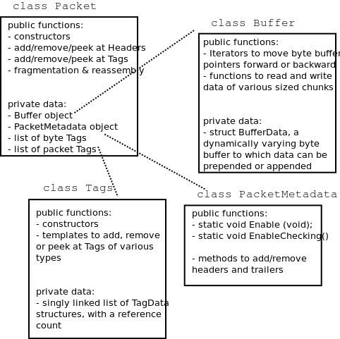
Implementation overview of Packet class.
Figure Implementation overview of Packet class. is a high-level overview of the Packet implementation; more detail on the byte Buffer implementation is provided later in Figure Implementation overview of a packet’s byte Buffer.. In ns-3, the Packet byte buffer is analogous to a Linux skbuff or BSD mbuf; it is a serialized representation of the actual data in the packet. The tag lists are containers for extra items useful for simulation convenience; if a Packet is converted to an emulated packet and put over an actual network, the tags are stripped off and the byte buffer is copied directly into a real packet.
Packets are reference counted objects. They are handled with smart pointer (Ptr) objects like many of the objects in the ns-3 system. One small difference you will see is that class Packet does not inherit from class Object or class RefCountBase, and implements the Ref() and Unref() methods directly. This was designed to avoid the overhead of a vtable in class Packet.
The Packet class is designed to be copied cheaply; the overall design is based on Copy on Write (COW). When there are multiple references to a packet object, and there is an operation on one of them, only so-called “dirty” operations will trigger a deep copy of the packet:
- ns3::Packet::AddHeader()
- ns3::Packet::AddTrailer()
- both versions of ns3::Packet::AddAtEnd()
- Packet::RemovePacketTag()
The fundamental classes for adding to and removing from the byte buffer are class Header and class Trailer. Headers are more common but the below discussion also largely applies to protocols using trailers. Every protocol header that needs to be inserted and removed from a Packet instance should derive from the abstract Header base class and implement the private pure virtual methods listed below:
- ns3::Header::SerializeTo()
- ns3::Header::DeserializeFrom()
- ns3::Header::GetSerializedSize()
- ns3::Header::PrintTo()
Basically, the first three functions are used to serialize and deserialize protocol control information to/from a Buffer. For example, one may define class TCPHeader : public Header. The TCPHeader object will typically consist of some private data (like a sequence number) and public interface access functions (such as checking the bounds of an input). But the underlying representation of the TCPHeader in a Packet Buffer is 20 serialized bytes (plus TCP options). The TCPHeader::SerializeTo() function would therefore be designed to write these 20 bytes properly into the packet, in network byte order. The last function is used to define how the Header object prints itself onto an output stream.
Similarly, user-defined Tags can be appended to the packet. Unlike Headers, Tags are not serialized into a contiguous buffer but are stored in lists. Tags can be flexibly defined to be any type, but there can only be one instance of any particular object type in the Tags buffer at any time.
Using the packet interface
This section describes how to create and use the ns3::Packet object.
Creating a new packet
The following command will create a new packet with a new unique Id.:
Ptr<Packet> pkt = Create<Packet> ();
What is the Uid (unique Id)? It is an internal id that the system uses to identify packets. It can be fetched via the following method::
uint32_t uid = pkt->GetUid ();
But please note the following. This uid is an internal uid and cannot be counted on to provide an accurate counter of how many “simulated packets” of a particular protocol are in the system. It is not trivial to make this uid into such a counter, because of questions such as what should the uid be when the packet is sent over broadcast media, or when fragmentation occurs. If a user wants to trace actual packet counts, he or she should look at e.g. the IP ID field or transport sequence numbers, or other packet or frame counters at other protocol layers.
We mentioned above that it is possible to create packets with zero-filled payloads that do not actually require a memory allocation (i.e., the packet may behave, when delays such as serialization or transmission delays are computed, to have a certain number of payload bytes, but the bytes will only be allocated on-demand when needed). The command to do this is, when the packet is created::
Ptr<Packet> pkt = Create<Packet> (N);
where N is a positive integer.
The packet now has a size of N bytes, which can be verified by the GetSize() method::
/**
 * \returns the size in bytes of the packet (including the zero-filled
 *          initial payload)
 */
uint32_t GetSize (void) const;
You can also initialize a packet with a character buffer. The input data is copied and the input buffer is untouched. The constructor applied is::
Packet (uint8_t const *buffer, uint32_t size);
Here is an example::
Ptr<Packet> pkt1 = Create<Packet> (reinterpret_cast<const uint8_t*> ("hello"), 5);
Packets are freed when there are no more references to them, as with all ns-3 objects referenced by the Ptr class.
Adding and removing Buffer data
After the initial packet creation (which may possibly create some fake initial bytes of payload), all subsequent buffer data is added by adding objects of class Header or class Trailer. Note that, even if you are in the application layer, handling packets, and want to write application data, you write it as an ns3::Header or ns3::Trailer. If you add a Header, it is prepended to the packet, and if you add a Trailer, it is added to the end of the packet. If you have no data in the packet, then it makes no difference whether you add a Header or Trailer. Since the APIs and classes for header and trailer are pretty much identical, we’ll just look at class Header here.
The first step is to create a new header class. All new Header classes must inherit from class Header, and implement the following methods:
- Serialize ()
- Deserialize ()
- GetSerializedSize ()
- Print ()
To see a simple example of how these are done, look at the UdpHeader class headers src/internet-stack/udp-header.cc. There are many other examples within the source code.
Once you have a header (or you have a preexisting header), the following Packet API can be used to add or remove such headers.:
/**
 * Add header to this packet. This method invokes the
 * Header::GetSerializedSize and Header::Serialize
 * methods to reserve space in the buffer and request the
 * header to serialize itself in the packet buffer.
 *
 * \param header a reference to the header to add to this packet.
 */
void AddHeader (const Header & header);
/**
 * Deserialize and remove the header from the internal buffer.
 * This method invokes Header::Deserialize.
 *
 * \param header a reference to the header to remove from the internal buffer.
 * \returns the number of bytes removed from the packet.
 */
uint32_t RemoveHeader (Header &header);
/**
 * Deserialize but does _not_ remove the header from the internal buffer.
 * This method invokes Header::Deserialize.
 *
 * \param header a reference to the header to read from the internal buffer.
 * \returns the number of bytes read from the packet.
 */
uint32_t PeekHeader (Header &header) const;
For instance, here are the typical operations to add and remove a UDP header.:
// add header
Ptr<Packet> packet = Create<Packet> ();
UdpHeader udpHeader;
// Fill out udpHeader fields appropriately
packet->AddHeader (udpHeader);
...
// remove header
UdpHeader udpHeader;
packet->RemoveHeader (udpHeader);
// Read udpHeader fields as needed
Adding and removing Tags
There is a single base class of Tag that all packet tags must derive from. They are used in two different tag lists in the packet; the lists have different semantics and different expected use cases.
As the names imply, ByteTags follow bytes and PacketTags follow packets. What this means is that when operations are done on packets, such as fragmentation, concatenation, and appending or removing headers, the byte tags keep track of which packet bytes they cover. For instance, if a user creates a TCP segment, and applies a ByteTag to the segment, each byte of the TCP segment will be tagged. However, if the next layer down inserts an IPv4 header, this ByteTag will not cover those bytes. The converse is true for the PacketTag; it covers a packet despite the operations on it.
PacketTags are limited in size to 20 bytes. This is a modifiable compile-time constant in src/common/packet-tag-list.h. ByteTags have no such restriction.
Each tag type must subclass ns3::Tag, and only one instance of each Tag type may be in each tag list. Here are a few differences in the behavior of packet tags and byte tags.
- Fragmentation: As mentioned above, when a packet is fragmented, each packet fragment (which is a new packet) will get a copy of all packet tags, and byte tags will follow the new packet boundaries (i.e. if the fragmented packets fragment across a buffer region covered by the byte tag, both packet fragments will still have the appropriate buffer regions byte tagged).
- Concatenation: When packets are combined, two different buffer regions will become one. For byte tags, the byte tags simply follow the respective buffer regions. For packet tags, only the tags on the first packet survive the merge.
- Finding and Printing: Both classes allow you to iterate over all of the tags and print them.
- Removal: Users can add and remove the same packet tag multiple times on a single packet (AddPacketTag () and RemovePacketTag ()). The packet However, once a byte tag is added, it can only be removed by stripping all byte tags from the packet. Removing one of possibly multiple byte tags is not supported by the current API.
As of ns-3.5 and later, Tags are not serialized and deserialized to a buffer when Packet::Serialize () and Packet::Deserialize () are called; this is an open bug.
If a user wants to take an existing packet object and reuse it as a new packet, he or she should remove all byte tags and packet tags before doing so. An example is the UdpEchoServer class, which takes the received packet and “turns it around” to send back to the echo client.
The Packet API for byte tags is given below.:
/**
 * \param tag the new tag to add to this packet
 *
 * Tag each byte included in this packet with the
 * new tag.
 *
 * Note that adding a tag is a const operation which is pretty
 * un-intuitive. The rationale is that the content and behavior of
 * a packet is _not_ changed when a tag is added to a packet: any
 * code which was not aware of the new tag is going to work just
 * the same if the new tag is added. The real reason why adding a
 * tag was made a const operation is to allow a trace sink which gets
 * a packet to tag the packet, even if the packet is const (and most
 * trace sources should use const packets because it would be
 * totally evil to allow a trace sink to modify the content of a
 * packet).
 */
void AddByteTag (const Tag &tag) const;
/**
 * \returns an iterator over the set of byte tags included in this packet.
 */
ByteTagIterator GetByteTagIterator (void) const;
/**
 * \param tag the tag to search in this packet
 * \returns true if the requested tag type was found, false otherwise.
 *
 * If the requested tag type is found, it is copied in the user's
 * provided tag instance.
 */
bool FindFirstMatchingByteTag (Tag &tag) const;

/**
 * Remove all the tags stored in this packet.
 */
void RemoveAllByteTags (void);

/**
 * \param os output stream in which the data should be printed.
 *
 * Iterate over the tags present in this packet, and
 * invoke the Print method of each tag stored in the packet.
 */
void PrintByteTags (std::ostream &os) const;
The Packet API for packet tags is given below.:
/**
 * \param tag the tag to store in this packet
 *
 * Add a tag to this packet. This method calls the
 * Tag::GetSerializedSize and, then, Tag::Serialize.
 *
 * Note that this method is const, that is, it does not
 * modify the state of this packet, which is fairly
 * un-intuitive.
 */
void AddPacketTag (const Tag &tag) const;
/**
 * \param tag the tag to remove from this packet
 * \returns true if the requested tag is found, false
 *          otherwise.
 *
 * Remove a tag from this packet. This method calls
 * Tag::Deserialize if the tag is found.
 */
bool RemovePacketTag (Tag &tag);
/**
 * \param tag the tag to search in this packet
 * \returns true if the requested tag is found, false
 *          otherwise.
 *
 * Search a matching tag and call Tag::Deserialize if it is found.
 */
bool PeekPacketTag (Tag &tag) const;
/**
 * Remove all packet tags.
 */
void RemoveAllPacketTags (void);

/**
 * \param os the stream in which we want to print data.
 *
 * Print the list of 'packet' tags.
 *
 * \sa Packet::AddPacketTag, Packet::RemovePacketTag, Packet::PeekPacketTag,
 *  Packet::RemoveAllPacketTags
 */
void PrintPacketTags (std::ostream &os) const;

/**
 * \returns an object which can be used to iterate over the list of
 *  packet tags.
 */
PacketTagIterator GetPacketTagIterator (void) const;
Here is a simple example illustrating the use of tags from the code in src/internet-stack/udp-socket-impl.cc::
Ptr<Packet> p;  // pointer to a pre-existing packet
SocketIpTtlTag tag
tag.SetTtl (m_ipMulticastTtl); // Convey the TTL from UDP layer to IP layer
p->AddPacketTag (tag);
This tag is read at the IP layer, then stripped (src/internet-stack/ipv4-l3-protocol.cc)::
uint8_t ttl = m_defaultTtl;
SocketIpTtlTag tag;
bool found = packet->RemovePacketTag (tag);
if (found)
  {
    ttl = tag.GetTtl ();
  }
Fragmentation and concatenation
Packets may be fragmented or merged together. For example, to fragment a packet p of 90 bytes into two packets, one containing the first 10 bytes and the other containing the remaining 80, one may call the following code::
Ptr<Packet> frag0 = p->CreateFragment (0, 10);
Ptr<Packet> frag1 = p->CreateFragment (10, 90);
As discussed above, the packet tags from p will follow to both packet fragments, and the byte tags will follow the byte ranges as needed.
Now, to put them back together::
frag0->AddAtEnd (frag1);
Now frag0 should be equivalent to the original packet p. If, however, there were operations on the fragments before being reassembled (such as tag operations or header operations), the new packet will not be the same.
Enabling metadata
We mentioned above that packets, being on-the-wire representations of byte buffers, present a problem to print out in a structured way unless the printing function has access to the context of the header. For instance, consider a tcpdump-like printer that wants to pretty-print the contents of a packet.
To enable this usage, packets may have metadata enabled (disabled by default for performance reasons). This class is used by the Packet class to record every operation performed on the packet’s buffer, and provides an implementation of Packet::Print () method that uses the metadata to analyze the content of the packet’s buffer.
The metadata is also used to perform extensive sanity checks at runtime when performing operations on a Packet. For example, this metadata is used to verify that when you remove a header from a packet, this same header was actually present at the front of the packet. These errors will be detected and will abort the program.
To enable this operation, users will typically insert one or both of these statements at the beginning of their programs::
Packet::EnablePrinting ();
Packet::EnableChecking ();
Sample programs
See samples/main-packet.cc and samples/main-packet-tag.cc.
Implementation details
Private member variables
A Packet object’s interface provides access to some private data::
Buffer m_buffer;
ByteTagList m_byteTagList;
PacketTagList m_packetTagList;
PacketMetadata m_metadata;
mutable uint32_t m_refCount;
static uint32_t m_globalUid;
Each Packet has a Buffer and two Tags lists, a PacketMetadata object, and a ref count. A static member variable keeps track of the UIDs allocated. The actual uid of the packet is stored in the PacketMetadata.
Note: that real network packets do not have a UID; the UID is therefore an instance of data that normally would be stored as a Tag in the packet. However, it was felt that a UID is a special case that is so often used in simulations that it would be more convenient to store it in a member variable.
Buffer implementation
Class Buffer represents a buffer of bytes. Its size is automatically adjusted to hold any data prepended or appended by the user. Its implementation is optimized to ensure that the number of buffer resizes is minimized, by creating new Buffers of the maximum size ever used. The correct maximum size is learned at runtime during use by recording the maximum size of each packet.
Authors of new Header or Trailer classes need to know the public API of the Buffer class. (add summary here)
The byte buffer is implemented as follows:
struct BufferData {
    uint32_t m_count;
    uint32_t m_size;
    uint32_t m_initialStart;
    uint32_t m_dirtyStart;
    uint32_t m_dirtySize;
    uint8_t m_data[1];
};
struct BufferData *m_data;
uint32_t m_zeroAreaSize;
uint32_t m_start;
uint32_t m_size;
- BufferData::m_count: reference count for BufferData structure
- BufferData::m_size: size of data buffer stored in BufferData structure
- BufferData::m_initialStart: offset from start of data buffer where data was first inserted
- BufferData::m_dirtyStart: offset from start of buffer where every Buffer which holds a reference to this BufferData instance have written data so far
- BufferData::m_dirtySize: size of area where data has been written so far
- BufferData::m_data: pointer to data buffer
- Buffer::m_zeroAreaSize: size of zero area which extends before m_initialStart
- Buffer::m_start: offset from start of buffer to area used by this buffer
- Buffer::m_size: size of area used by this Buffer in its BufferData structure
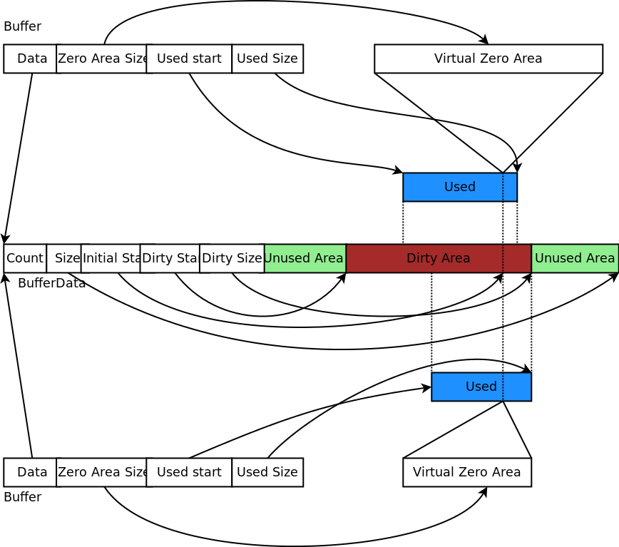
Implementation overview of a packet’s byte Buffer.
This data structure is summarized in Figure Implementation overview of a packet’s byte Buffer.. Each Buffer holds a pointer to an instance of a BufferData. Most Buffers should be able to share the same underlying BufferData and thus simply increase the BufferData’s reference count. If they have to change the content of a BufferData inside the Dirty Area, and if the reference count is not one, they first create a copy of the BufferData and then complete their state-changing operation.
Tags implementation
(XXX revise me)
Tags are implemented by a single pointer which points to the start of a linked list ofTagData data structures. Each TagData structure points to the next TagData in the list (its next pointer contains zero to indicate the end of the linked list). Each TagData contains an integer unique id which identifies the type of the tag stored in the TagData.:
struct TagData {
    struct TagData *m_next;
    uint32_t m_id;
    uint32_t m_count;
    uint8_t m_data[Tags::SIZE];
};
class Tags {
    struct TagData *m_next;
};
Adding a tag is a matter of inserting a new TagData at the head of the linked list. Looking at a tag requires you to find the relevant TagData in the linked list and copy its data into the user data structure. Removing a tag and updating the content of a tag requires a deep copy of the linked list before performing this operation. On the other hand, copying a Packet and its tags is a matter of copying the TagData head pointer and incrementing its reference count.
Tags are found by the unique mapping between the Tag type and its underlying id. This is why at most one instance of any Tag can be stored in a packet. The mapping between Tag type and underlying id is performed by a registration as follows::
/* A sample Tag implementation
 */
struct MyTag {
    uint16_t m_streamId;
};
Memory management
Describe dataless vs. data-full packets.
Copy-on-write semantics
The current implementation of the byte buffers and tag list is based on COW (Copy On Write). An introduction to COW can be found in Scott Meyer’s “More Effective C++”, items 17 and 29). This design feature and aspects of the public interface borrows from the packet design of the Georgia Tech Network Simulator. This implementation of COW uses a customized reference counting smart pointer class.
What COW means is that copying packets without modifying them is very cheap (in terms of CPU and memory usage) and modifying them can be also very cheap. What is key for proper COW implementations is being able to detect when a given modification of the state of a packet triggers a full copy of the data prior to the modification: COW systems need to detect when an operation is “dirty” and must therefore invoke a true copy.
Dirty operations:
- ns3::Packet::AddHeader
- ns3::Packet::AddTrailer
- both versions of ns3::Packet::AddAtEnd
- ns3::Packet::RemovePacketTag
Non-dirty operations:
- ns3::Packet::AddPacketTag
- ns3::Packet::PeekPacketTag
- ns3::Packet::RemoveAllPacketTags
- ns3::Packet::AddByteTag
- ns3::Packet::FindFirstMatchingByteTag
- ns3::Packet::RemoveAllByteTags
- ns3::Packet::RemoveHeader
- ns3::Packet::RemoveTrailer
- ns3::Packet::CreateFragment
- ns3::Packet::RemoveAtStart
- ns3::Packet::RemoveAtEnd
- ns3::Packet::CopyData
Dirty operations will always be slower than non-dirty operations, sometimes by several orders of magnitude. However, even the dirty operations have been optimized for common use-cases which means that most of the time, these operations will not trigger data copies and will thus be still very fast.
Helpers
The above chapters introduced you to various ns-3 programming concepts such as smart pointers for reference-counted memory management, attributes, namespaces, callbacks, etc. Users who work at this low-level API can interconnect ns-3 objects with fine granulariy. However, a simulation program written entirely using the low-level API would be quite long and tedious to code. For this reason, a separate so-called “helper API” has been overlaid on the core ns-3 API. If you have read the ns-3 tutorial, you will already be familiar with the helper API, since it is the API that new users are typically introduced to first. In this chapter, we introduce the design philosophy of the helper API and contrast it to the low-level API. If you become a heavy user of ns-3, you will likely move back and forth between these APIs even in the same program.
The helper API has a few goals:
- the rest of src/ has no dependencies on the helper API; anything that can be done with the helper API can be coded also at the low-level API
- Containers: Often simulations will need to do a number of identical actions to groups of objects. The helper API makes heavy use of containers of similar objects to which similar or identical operations can be performed.
- The helper API is not generic; it does not strive to maximize code reuse. So, programming constructs such as polymorphism and templates that achieve code reuse are not as prevalent. For instance, there are separate CsmaNetDevice helpers and PointToPointNetDevice helpers but they do not derive from a common NetDevice base class.
- The helper API typically works with stack-allocated (vs. heap-allocated) objects. For some programs, ns-3 users may not need to worry about any low level Object Create or Ptr handling; they can make do with containers of objects and stack-allocated helpers that operate on them.
The helper API is really all about making ns-3 programs easier to write and read, without taking away the power of the low-level interface. The rest of this chapter provides some examples of the programming conventions of the helper API.
Python
Placeholder chapter
For now, please see the Python wiki page at http://www.nsnam.org/wiki/index.php/NS-3_Python_Bindings.
Node and NetDevices
Node and NetDevices Overview
This chapter describes how ns-3 nodes are put together, and provides a walk-through of how packets traverse an internet-based Node.
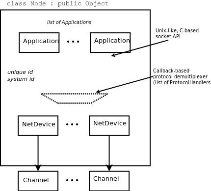
High-level node architecture
In ns-3, nodes are instances of ns3::Node. This class may be subclassed, but instead, the conceptual model is that we aggregate or insert objects to it rather than define subclasses.
One might think of a bare ns-3 node as a shell of a computer, to which one may add NetDevices (cards) and other innards including the protocols and applications. High-level node architecture illustrates that ns3::Node objects contain a list of ns3::Application instances (initially, the list is empty), a list of ns3::NetDevice instances (initially, the list is empty), a list of ns3::Node::ProtocolHandler instances, a unique integer ID, and a system ID (for distributed simulation).
The design tries to avoid putting too many dependencies on the class ns3::Node, ns3::Application, or ns3::NetDevice for the following:
- IP version, or whether IP is at all even used in the ns3::Node.
- implementation details of the IP stack.
From a software perspective, the lower interface of applications corresponds to the C-based sockets API. The upper interface of ns3::NetDevice objects corresponds to the device independent sublayer of the Linux stack. Everything in between can be aggregated and plumbed together as needed.
Let’s look more closely at the protocol demultiplexer. We want incoming frames at layer-2 to be delivered to the right layer-3 protocol such as IPv4. The function of this demultiplexer is to register callbacks for receiving packets. The callbacks are indexed based on the EtherType in the layer-2 frame.
Many different types of higher-layer protocols may be connected to the NetDevice, such as IPv4, IPv6, ARP, MPLS, IEEE 802.1x, and packet sockets. Therefore, the use of a callback-based demultiplexer avoids the need to use a common base class for all of these protocols, which is problematic because of the different types of objects (including packet sockets) expected to be registered there.
Simple NetDevice
Placeholder chapter
PointToPoint NetDevice
This is the introduction to PointToPoint NetDevice chapter, to complement the PointToPoint model doxygen.
Overview of the PointToPoint model
The ns-3 point-to-point model is of a very simple point to point data link connecting exactly two PointToPointNetDevice devices over an PointToPointChannel. This can be viewed as equivalent to a full duplex RS-232 or RS-422 link with null modem and no handshaking.
Data is encapsulated in the Point-to-Point Protocol (PPP – RFC 1661), however the Link Control Protocol (LCP) and associated state machine is not implemented. The PPP link is assumed to be established and authenticated at all times.
Data is not framed, therefore Address and Control fields will not be found. Since the data is not framed, there is no need to provide Flag Sequence and Control Escape octets, nor is a Frame Check Sequence appended. All that is required to implement non-framed PPP is to prepend the PPP protocol number for IP Version 4 which is the sixteen-bit number 0x21 (see http://www.iana.org/assignments/ppp-numbers).
The PointToPointNetDevice provides following Attributes:
- Address: The ns3::Mac48Address of the device (if desired);
- DataRate: The data rate (ns3::DataRate) of the device;
- TxQueue: The transmit queue (ns3::Queue) used by the device;
- InterframeGap: The optional ns3::Time to wait between “frames”;
- Rx: A trace source for received packets;
- Drop: A trace source for dropped packets.
The PointToPointNetDevice models a transmitter section that puts bits on a corresponding channel “wire.” The DataRate attribute specifies the number of bits per second that the device will simulate sending over the channel. In reality no bits are sent, but an event is scheduled for an elapsed time consistent with the number of bits in each packet and the specified DataRate. The implication here is that the receiving device models a receiver section that can receive any any data rate. Therefore there is no need, nor way to set a receive data rate in this model. By setting the DataRate on the transmitter of both devices connected to a given PointToPointChannel one can model a symmetric channel; or by setting different DataRates one can model an asymmetric channel (e.g., ADSL).
The PointToPointNetDevice supports the assignment of a “receive error model.” This is an ErrorModel object that is used to simulate data corruption on the link.
Point-to-Point Channel Model
The point to point net devices are connected via an PointToPointChannel. This channel models two wires transmitting bits at the data rate specified by the source net device. There is no overhead beyond the eight bits per byte of the packet sent. That is, we do not model Flag Sequences, Frame Check Sequences nor do we “escape” any data.
The PointToPointChannel provides following Attributes:
- Delay: An ns3::Time specifying the speed of light transmission delay for the channel.
Using the PointToPointNetDevice
The PointToPoint net devices and channels are typically created and configured using the associated PointToPointHelper object. The various ns3 device helpers generally work in a similar way, and their use is seen in many of our example programs and is also covered in the ns-3 tutorial.
The conceptual model of interest is that of a bare computer “husk” into which you plug net devices. The bare computers are created using a NodeContainer helper. You just ask this helper to create as many computers (we call them Nodes) as you need on your network::
NodeContainer nodes;
nodes.Create (2);
Once you have your nodes, you need to instantiate a PointToPointHelper and set any attributes you may want to change. Note that since this is a point-to-point (as compared to a point-to-multipoint) there may only be two nodes with associated net devices connected by a PointToPointChannel.:
PointToPointHelper pointToPoint;
pointToPoint.SetDeviceAttribute ("DataRate", StringValue ("5Mbps"));
pointToPoint.SetChannelAttribute ("Delay", StringValue ("2ms"));
Once the attributes are set, all that remains is to create the devices and install them on the required nodes, and to connect the devices together using a PointToPoint channel. When we create the net devices, we add them to a container to allow you to use them in the future. This all takes just one line of code.:
NetDeviceContainer devices = pointToPoint.Install (nodes);
PointToPoint Tracing
Like all ns-3 devices, the Point-to-Point Model provides a number of trace sources. These trace sources can be hooked using your own custom trace code, or you can use our helper functions to arrange for tracing to be enabled on devices you specify.
Upper-Level (MAC) Hooks
From the point of view of tracing in the net device, there are several interesting points to insert trace hooks. A convention inherited from other simulators is that packets destined for transmission onto attached networks pass through a single “transmit queue” in the net device. We provide trace hooks at this point in packet flow, which corresponds (abstractly) only to a transition from the network to data link layer, and call them collectively the device MAC hooks.
When a packet is sent to the Point-to-Point net device for transmission it always passes through the transmit queue. The transmit queue in the PointToPointNetDevice inherits from Queue, and therefore inherits three trace sources::
* An Enqueue operation source (see ns3::Queue::m_traceEnqueue);
* A Dequeue operation source (see ns3::Queue::m_traceDequeue);
* A Drop operation source (see ns3::Queue::m_traceDrop).
The upper-level (MAC) trace hooks for the PointToPointNetDevice are, in fact, exactly these three trace sources on the single transmit queue of the device.
The m_traceEnqueue event is triggered when a packet is placed on the transmit queue. This happens at the time that ns3::PointtoPointNetDevice::Send or ns3::PointToPointNetDevice::SendFrom is called by a higher layer to queue a packet for transmission. An Enqueue trace event firing should be interpreted as only indicating that a higher level protocol has sent a packet to the device.
The m_traceDequeue event is triggered when a packet is removed from the transmit queue. Dequeues from the transmit queue can happen in two situations: 1) If the underlying channel is idle when PointToPointNetDevice::Send is called, a packet is dequeued from the transmit queue and immediately transmitted; 2) a packet may be dequeued and immediately transmitted in an internal TransmitCompleteEvent that functions much like a transmit complete interrupt service routine. An Dequeue trace event firing may be viewed as indicating that the PointToPointNetDevice has begun transmitting a packet.
Lower-Level (PHY) Hooks
Similar to the upper level trace hooks, there are trace hooks available at the lower levels of the net device. We call these the PHY hooks. These events fire from the device methods that talk directly to the PointToPointChannel.
The trace source m_dropTrace is called to indicate a packet that is dropped by the device. This happens when a packet is discarded as corrupt due to a receive error model indication (see ns3::ErrorModel and the associated attribute “ReceiveErrorModel”).
The other low-level trace source fires on reception of a packet (see ns3::PointToPointNetDevice::m_rxTrace) from the PointToPointChannel.
CSMA NetDevice
This is the introduction to CSMA NetDevice chapter, to complement the Csma model doxygen.
Overview of the CSMA model
The ns-3 CSMA device models a simple bus network in the spirit of Ethernet. Although it does not model any real physical network you could ever build or buy, it does provide some very useful functionality.
Typically when one thinks of a bus network Ethernet or IEEE 802.3 comes to mind. Ethernet uses CSMA/CD (Carrier Sense Multiple Access with Collision Detection with exponentially increasing backoff to contend for the shared transmission medium. The ns-3 CSMA device models only a portion of this process, using the nature of the globally available channel to provide instantaneous (faster than light) carrier sense and priority-based collision “avoidance.” Collisions in the sense of Ethernet never happen and so the ns-3 CSMA device does not model collision detection, nor will any transmission in progress be “jammed.”
CSMA Layer Model
There are a number of conventions in use for describing layered communications architectures in the literature and in textbooks. The most common layering model is the ISO seven layer reference model. In this view the CsmaNetDevice and CsmaChannel pair occupies the lowest two layers – at the physical (layer one), and data link (layer two) positions. Another important reference model is that specified by RFC 1122, “Requirements for Internet Hosts – Communication Layers.” In this view the CsmaNetDevice and CsmaChannel pair occupies the lowest layer – the link layer. There is also a seemingly endless litany of alternative descriptions found in textbooks and in the literature. We adopt the naming conventions used in the IEEE 802 standards which speak of LLC, MAC, MII and PHY layering. These acronyms are defined as:
- LLC: Logical Link Control;
- MAC: Media Access Control;
- MII: Media Independent Interface;
- PHY: Physical Layer.
In this case the LLC and MAC are sublayers of the OSI data link layer and the MII and PHY are sublayers of the OSI physical layer.
The “top” of the CSMA device defines the transition from the network layer to the data link layer. This transition is performed by higher layers by calling either CsmaNetDevice::Send or CsmaNetDevice::SendFrom.
In contrast to the IEEE 802.3 standards, there is no precisely specified PHY in the CSMA model in the sense of wire types, signals or pinouts. The “bottom” interface of the CsmaNetDevice can be thought of as as a kind of Media Independent Interface (MII) as seen in the “Fast Ethernet” (IEEE 802.3u) specifications. This MII interface fits into a corresponding media independent interface on the CsmaChannel. You will not find the equivalent of a 10BASE-T or a 1000BASE-LX PHY.
The CsmaNetDevice calls the CsmaChannel through a media independent interface. There is a method defined to tell the channel when to start “wiggling the wires” using the method CsmaChannel::TransmitStart, and a method to tell the channel when the transmission process is done and the channel should begin propagating the last bit across the “wire”: CsmaChannel::TransmitEnd.
When the TransmitEnd method is executed, the channel will model a single uniform signal propagation delay in the medium and deliver copes of the packet to each of the devices attached to the packet via the CsmaNetDevice::Receive method.
There is a “pin” in the device media independent interface corresponding to “COL” (collision). The state of the channel may be sensed by calling CsmaChannel::GetState. Each device will look at this “pin” before starting a send and will perform appropriate backoff operations if required.
Properly received packets are forwarded up to higher levels from the CsmaNetDevice via a callback mechanism. The callback function is initialized by the higher layer (when the net device is attached) using CsmaNetDevice::SetReceiveCallback and is invoked upon “proper” reception of a packet by the net device in order to forward the packet up the protocol stack.
CSMA Channel Model
The class CsmaChannel models the actual transmission medium. There is no fixed limit for the number of devices connected to the channel. The CsmaChannel models a data rate and a speed-of-light delay which can be accessed via the attributes “DataRate” and “Delay” respectively. The data rate provided to the channel is used to set the data rates used by the transmitter sections of the CSMA devices connected to the channel. There is no way to independently set data rates in the devices. Since the data rate is only used to calculate a delay time, there is no limitation (other than by the data type holding the value) on the speed at which CSMA channels and devices can operate; and no restriction based on any kind of PHY characteristics.
The CsmaChannel has three states, IDLE, TRANSMITTING and PROPAGATING. These three states are “seen” instantaneously by all devices on the channel. By this we mean that if one device begins or ends a simulated transmission, all devices on the channel are immediately aware of the change in state. There is no time during which one device may see an IDLE channel while another device physically further away in the collision domain may have begun transmitting with the associated signals not propagated down the channel to other devices. Thus there is no need for collision detection in the CsmaChannel model and it is not implemented in any way.
We do, as the name indicates, have a Carrier Sense aspect to the model. Since the simulator is single threaded, access to the common channel will be serialized by the simulator. This provides a deterministic mechanism for contending for the channel. The channel is allocated (transitioned from state IDLE to state TRANSMITTING) on a first-come first-served basis. The channel always goes through a three state process::
IDLE -> TRANSMITTING -> PROPAGATING -> IDLE
The TRANSMITTING state models the time during which the source net device is actually wiggling the signals on the wire. The PROPAGATING state models the time after the last bit was sent, when the signal is propagating down the wire to the “far end.”
The transition to the TRANSMITTING state is driven by a call to CsmaChannel::TransmitStart which is called by the net device that transmits the packet. It is the responsibility of that device to end the transmission with a call to CsmaChannel::TransmitEnd at the appropriate simulation time that reflects the time elapsed to put all of the packet bits on the wire. When TransmitEnd is called, the channel schedules an event corresponding to a single speed-of-light delay. This delay applies to all net devices on the channel identically. You can think of a symmetrical hub in which the packet bits propagate to a central location and then back out equal length cables to the other devices on the channel. The single “speed of light” delay then corresponds to the time it takes for: 1) a signal to propagate from one CsmaNetDevice through its cable to the hub; plus 2) the time it takes for the hub to forward the packet out a port; plus 3) the time it takes for the signal in question to propagate to the destination net device.
The CsmaChannel models a broadcast medium so the packet is delivered to all of the devices on the channel (including the source) at the end of the propagation time. It is the responsibility of the sending device to determine whether or not it receives a packet broadcast over the channel.
The CsmaChannel provides following Attributes:
- DataRate: The bitrate for packet transmission on connected devices;
- Delay: The speed of light transmission delay for the channel.
CSMA Net Device Model
The CSMA network device appears somewhat like an Ethernet device. The CsmaNetDevice provides following Attributes:
- Address: The Mac48Address of the device;
- SendEnable: Enable packet transmission if true;
- ReceiveEnable: Enable packet reception if true;
- EncapsulationMode: Type of link layer encapsulation to use;
- RxErrorModel: The receive error model;
- TxQueue: The transmit queue used by the device;
- InterframeGap: The optional time to wait between “frames”;
- Rx: A trace source for received packets;
- Drop: A trace source for dropped packets.
The CsmaNetDevice supports the assignment of a “receive error model.” This is an ErrorModel object that is used to simulate data corruption on the link.
Packets sent over the CsmaNetDevice are always routed through the transmit queue to provide a trace hook for packets sent out over the network. This transmit queue can be set (via attribute) to model different queuing strategies.
Also configurable by attribute is the encapsulation method used by the device. Every packet gets an EthernetHeader that includes the destination and source MAC addresses, and a length/type field. Every packet also gets an EthernetTrailer which includes the FCS. Data in the packet may be encapsulated in different ways.
By default, or by setting the “EncapsulationMode” attribute to “Dix”, the encapsulation is according to the DEC, Intel, Xerox standard. This is sometimes called EthernetII framing and is the familiar destination MAC, source MAC, EtherType, Data, CRC format.
If the “EncapsulationMode” attribute is set to “Llc”, the encapsulation is by LLC SNAP. In this case, a SNAP header is added that contains the EtherType (IP or ARP).
The other implemented encapsulation modes are IP_ARP (set “EncapsulationMode” to “IpArp”) in which the length type of the Ethernet header receives the protocol number of the packet; or ETHERNET_V1 (set “EncapsulationMode” to “EthernetV1”) in which the length type of the Ethernet header receives the length of the packet. A “Raw” encapsulation mode is defined but not implemented – use of the RAW mode results in an assertion.
Note that all net devices on a channel must be set to the same encapsulation mode for correct results. The encapsulation mode is not sensed at the receiver.
The CsmaNetDevice implements a random exponential backoff algorithm that is executed if the channel is determined to be busy (TRANSMITTING or PPROPAGATING) when the device wants to start propagating. This results in a random delay of up to pow (2, retries) - 1 microseconds before a retry is attempted. The default maximum number of retries is 1000.
Using the CsmaNetDevice
The CSMA net devices and channels are typically created and configured using the associated CsmaHelper object. The various ns-3 device helpers generally work in a similar way, and their use is seen in many of our example programs.
The conceptual model of interest is that of a bare computer “husk” into which you plug net devices. The bare computers are created using a NodeContainer helper. You just ask this helper to create as many computers (we call them Nodes) as you need on your network::
NodeContainer csmaNodes;
csmaNodes.Create (nCsmaNodes);
Once you have your nodes, you need to instantiate a CsmaHelper and set any attributes you may want to change.:
CsmaHelper csma;
csma.SetChannelAttribute ("DataRate", StringValue ("100Mbps"));
csma.SetChannelAttribute ("Delay", TimeValue (NanoSeconds (6560)));

csma.SetDeviceAttribute ("EncapsulationMode", StringValue ("Dix"));
csma.SetDeviceAttribute ("FrameSize", UintegerValue (2000));
Once the attributes are set, all that remains is to create the devices and install them on the required nodes, and to connect the devices together using a CSMA channel. When we create the net devices, we add them to a container to allow you to use them in the future. This all takes just one line of code.:
NetDeviceContainer csmaDevices = csma.Install (csmaNodes);
CSMA Tracing
Like all ns-3 devices, the CSMA Model provides a number of trace sources. These trace sources can be hooked using your own custom trace code, or you can use our helper functions to arrange for tracing to be enabled on devices you specify.
Upper-Level (MAC) Hooks
From the point of view of tracing in the net device, there are several interesting points to insert trace hooks. A convention inherited from other simulators is that packets destined for transmission onto attached networks pass through a single “transmit queue” in the net device. We provide trace hooks at this point in packet flow, which corresponds (abstractly) only to a transition from the network to data link layer, and call them collectively the device MAC hooks.
When a packet is sent to the CSMA net device for transmission it always passes through the transmit queue. The transmit queue in the CsmaNetDevice inherits from Queue, and therefore inherits three trace sources:
- An Enqueue operation source (see Queue::m_traceEnqueue);
- A Dequeue operation source (see Queue::m_traceDequeue);
- A Drop operation source (see Queue::m_traceDrop).
The upper-level (MAC) trace hooks for the CsmaNetDevice are, in fact, exactly these three trace sources on the single transmit queue of the device.
The m_traceEnqueue event is triggered when a packet is placed on the transmit queue. This happens at the time that CsmaNetDevice::Send or CsmaNetDevice::SendFrom is called by a higher layer to queue a packet for transmission.
The m_traceDequeue event is triggered when a packet is removed from the transmit queue. Dequeues from the transmit queue can happen in three situations: 1) If the underlying channel is idle when the CsmaNetDevice::Send or CsmaNetDevice::SendFrom is called, a packet is dequeued from the transmit queue and immediately transmitted; 2) If the underlying channel is idle, a packet may be dequeued and immediately transmitted in an internal TransmitCompleteEvent that functions much like a transmit complete interrupt service routine; or 3) from the random exponential backoff handler if a timeout is detected.
Case (3) implies that a packet is dequeued from the transmit queue if it is unable to be transmitted according to the backoff rules. It is important to understand that this will appear as a Dequeued packet and it is easy to incorrectly assume that the packet was transmitted since it passed through the transmit queue. In fact, a packet is actually dropped by the net device in this case. The reason for this behavior is due to the definition of the Queue Drop event. The m_traceDrop event is, by definition, fired when a packet cannot be enqueued on the transmit queue because it is full. This event only fires if the queue is full and we do not overload this event to indicate that the CsmaChannel is “full.”
Lower-Level (PHY) Hooks
Similar to the upper level trace hooks, there are trace hooks available at the lower levels of the net device. We call these the PHY hooks. These events fire from the device methods that talk directly to the CsmaChannel.
The trace source m_dropTrace is called to indicate a packet that is dropped by the device. This happens in two cases: First, if the receive side of the net device is not enabled (see CsmaNetDevice::m_receiveEnable and the associated attribute “ReceiveEnable”).
The m_dropTrace is also used to indicate that a packet was discarded as corrupt if a receive error model is used (see CsmaNetDevice::m_receiveErrorModel and the associated attribute “ReceiveErrorModel”).
The other low-level trace source fires on reception of an accepted packet (see CsmaNetDevice::m_rxTrace). A packet is accepted if it is destined for the broadcast address, a multicast address, or to the MAC address assigned to the net device.
Wifi NetDevice
ns-3 nodes can contain a collection of NetDevice objects, much like an actual computer contains separate interface cards for Ethernet, Wifi, Bluetooth, etc. This chapter describes the ns-3 WifiNetDevice and related models. By adding WifiNetDevice objects to ns-3 nodes, one can create models of 802.11-based infrastructure and ad hoc networks.
Overview of the model
The WifiNetDevice models a wireless network interface controller based on the IEEE 802.11 standard. We will go into more detail below but in brief, ns-3 provides models for these aspects of 802.11:
- basic 802.11 DCF with infrastructure and adhoc modes
- 802.11a and 802.11b physical layers
- QoS-based EDCA and queueing extensions of 802.11e
- various propagation loss models including Nakagami, Rayleigh, Friis, LogDistance, FixedRss, Random
- two propagation delay models, a distance-based and random model
- various rate control algorithms including Aarf, Arf, Cara, Onoe, Rraa, ConstantRate, and Minstrel
- 802.11s (mesh), described in another chapter
The set of 802.11 models provided in ns-3 attempts to provide an accurate MAC-level implementation of the 802.11 specification and to provide a not-so-slow PHY-level model of the 802.11a specification.
The implementation is modular and provides roughly four levels of models:
- the PHY layer models
- the so-called MAC low models: they implement DCF and EDCAF
- the so-called MAC high models: they implement the MAC-level beacon generation, probing, and association state machines, and
- a set of Rate control algorithms used by the MAC low models
There are presently three MAC high models that provide for the three (non-mesh; the mesh equivalent, which is a sibling of these with common parent ns3::RegularWifiMac, is not discussed here) Wi-Fi topological elements - Access Point (AP) (implemented in class ns3::ApWifiMac, non-AP Station (STA) (ns3::StaWifiMac), and STA in an Independent Basic Service Set (IBSS - also commonly referred to as an ad hoc network (ns3::AdhocWifiMac).
The simplest of these is ns3::AdhocWifiMac`, which implements a Wi-Fi MAC that does not perform any kind of beacon generation, probing, or association. The ``ns3::StaWifiMac class implements an active probing and association state machine that handles automatic re-association whenever too many beacons are missed. Finally, ns3::ApWifiMac implements an AP that generates periodic beacons, and that accepts every attempt to associate.
These three MAC high models share a common parent in ns3::RegularWifiMac, which exposes, among other MAC configuration, an attribute QosSupported that allows configuration of 802.11e/WMM-style QoS support. With QoS-enabled MAC models it is possible to work with traffic belonging to four different Access Categories (ACs): AC_VO for voice traffic, AC_VI for video traffic, AC_BE for best-effort traffic and AC_BK for background traffic. In order for the MAC to determine the appropriate AC for an MSDU, packets forwarded down to these MAC layers should be marked using ns3::QosTag in order to set a TID (traffic id) for that packet otherwise it will be considered belonging to AC_BE.
The MAC low layer is split into three components:
- ns3::MacLow which takes care of RTS/CTS/DATA/ACK transactions.
- ns3::DcfManager and ns3::DcfState which implements the DCF and EDCAF functions.
- ns3::DcaTxop and ns3::EdcaTxopN which handle the packet queue, packet fragmentation, and packet retransmissions if they are needed. The ns3::DcaTxop object is used high MACs that are not QoS-enabled, and for transmission of frames (e.g., of type Management) that the standard says should access the medium using the DCF. ns3::EdcaTxopN is is used by QoS-enabled high MACs and also performs QoS operations like 802.11n-style MSDU aggregation.
There are also several rate control algorithms that can be used by the Mac low layer:
- ns3::ArfMacStations
- ns3::AArfMacStations
- ns3::IdealMacStations
- ns3::CrMacStations
- ns3::OnoeMacStations
- ns3::AmrrMacStations
The PHY layer implements a single model in the ns3::WifiPhy class: the physical layer model implemented there is described fully in a paper entitled Yet Another Network Simulator Validation results for 802.11b are available in this technical report
In ns-3, nodes can have multiple WifiNetDevices on separate channels, and the WifiNetDevice can coexist with other device types; this removes an architectural limitation found in ns-2. Presently, however, there is no model for cross-channel interference or coupling.
The source code for the Wifi NetDevice lives in the directory src/devices/wifi.
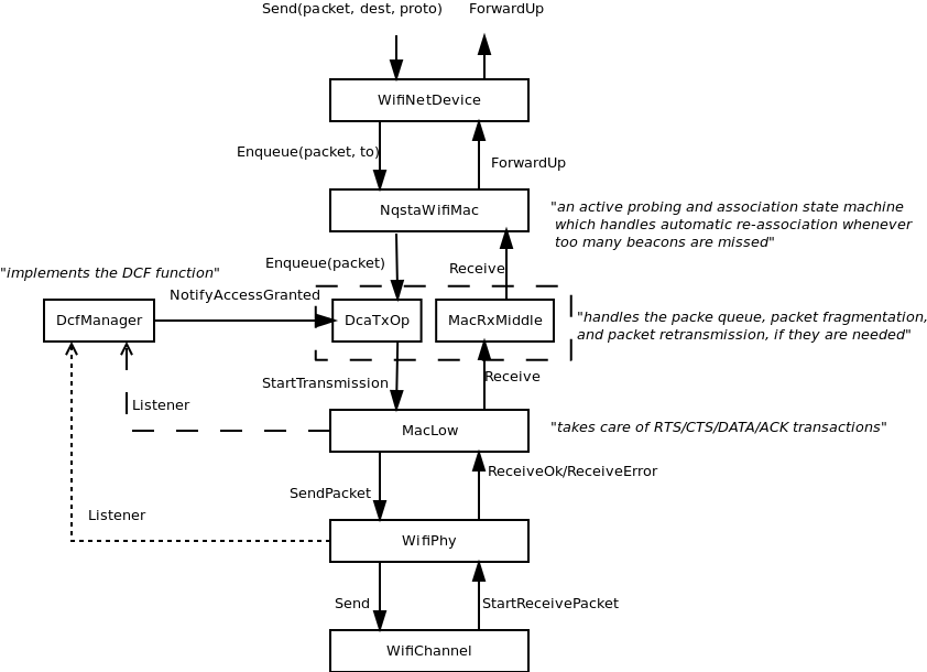
Wifi NetDevice architecture.
Using the WifiNetDevice
The modularity provided by the implementation makes low-level configuration of the WifiNetDevice powerful but complex. For this reason, we provide some helper classes to perform common operations in a simple matter, and leverage the ns-3 attribute system to allow users to control the parametrization of the underlying models.
Users who use the low-level ns-3 API and who wish to add a WifiNetDevice to their node must create an instance of a WifiNetDevice, plus a number of constituent objects, and bind them together appropriately (the WifiNetDevice is very modular in this regard, for future extensibility). At the low-level API, this can be done with about 20 lines of code (see ns3::WifiHelper::Install, and ns3::YansWifiPhyHelper::Create). They also must create, at some point, a WifiChannel, which also contains a number of constituent objects (see ns3::YansWifiChannelHelper::Create).
However, a few helpers are available for users to add these devices and channels with only a few lines of code, if they are willing to use defaults, and the helpers provide additional API to allow the passing of attribute values to change default values. The scripts in src/examples can be browsed to see how this is done.
YansWifiChannelHelper
The YansWifiChannelHelper has an unusual name. Readers may wonder why it is named this way. The reference is to the yans simulator from which this model is taken. The helper can be used to create a WifiChannel with a default PropagationLoss and PropagationDelay model. Specifically, the default is a channel model with a propagation delay equal to a constant, the speed of light, and a propagation loss based on a log distance model with a reference loss of 46.6777 dB at reference distance of 1m.
Users will typically type code such as::
YansWifiChannelHelper wifiChannelHelper = YansWifiChannelHelper::Default ();
Ptr<WifiChannel> wifiChannel = wifiChannelHelper.Create ();
to get the defaults. Note the distinction above in creating a helper object vs. an actual simulation object. In ns-3, helper objects (used at the helper API only) are created on the stack (they could also be created with operator new and later deleted). However, the actual ns-3 objects typically inherit from class ns3::Object and are assigned to a smart pointer. See the chapter on Object model for a discussion of the ns-3 object model, if you are not familiar with it.
Todo: Add notes about how to configure attributes with this helper API
YansWifiPhyHelper
Physical devices (base class ns3::Phy) connect to ns3::Channel models in ns-3. We need to create Phy objects appropriate for the YansWifiChannel; here the YansWifiPhyHelper will do the work.
The YansWifiPhyHelper class configures an object factory to create instances of a YansWifiPhy and adds some other objects to it, including possibly a supplemental ErrorRateModel and a pointer to a MobilityModel. The user code is typically::
YansWifiPhyHelper wifiPhyHelper = YansWifiPhyHelper::Default ();
wifiPhyHelper.SetChannel (wifiChannel);
Note that we haven’t actually created any WifiPhy objects yet; we’ve just prepared the YansWifiPhyHelper by telling it which channel it is connected to. The phy objects are created in the next step.
NqosWifiMacHelper and QosWifiMacHelper
The ns3::NqosWifiMacHelper and ns3::QosWifiMacHelper configure an object factory to create instances of a ns3::WifiMac. They are used to configure MAC parameters like type of MAC.
The former, ns3::NqosWifiMacHelper, supports creation of MAC instances that do not have 802.11e/WMM-style QoS support enabled.
For example the following user code configures a non-QoS MAC that will be a non-AP STA in an infrastructure network where the AP has SSID ns-3-ssid::
NqosWifiMacHelper wifiMacHelper = NqosWifiMacHelper::Default ();
Ssid ssid = Ssid ("ns-3-ssid");
wifiMacHelper.SetType ("ns3::StaWifiMac",
                      "Ssid", SsidValue (ssid),
                      "ActiveProbing", BooleanValue (false));
To create MAC instances with QoS support enabled, ns3::QosWifiMacHelper is used in place of ns3::NqosWifiMacHelper. This object can be also used to set:
- a MSDU aggregator for a particular Access Category (AC) in order to use 802.11n MSDU aggregation feature;
- block ack parameters like threshold (number of packets for which block ack mechanism should be used) and inactivity timeout.
The following code shows an example use of ns3::QosWifiMacHelper to create an AP with QoS enabled, aggregation on AC_VO, and Block Ack on AC_BE::
QosWifiMacHelper wifiMacHelper = QosWifiMacHelper::Default ();
wifiMacHelper.SetType ("ns3::ApWifiMac",
                       "Ssid", SsidValue (ssid),
                       "BeaconGeneration", BooleanValue (true),
                       "BeaconInterval", TimeValue (Seconds (2.5)));
wifiMacHelper.SetMsduAggregatorForAc (AC_VO, "ns3::MsduStandardAggregator",
                                      "MaxAmsduSize", UintegerValue (3839));
wifiMacHelper.SetBlockAckThresholdForAc (AC_BE, 10);
wifiMacHelper.SetBlockAckInactivityTimeoutForAc (AC_BE, 5);
WifiHelper
We’re now ready to create WifiNetDevices. First, let’s create a WifiHelper with default settings::
WifiHelper wifiHelper = WifiHelper::Default ();
What does this do? It sets the RemoteStationManager to ns3::ArfWifiManager. Now, let’s use the wifiPhyHelper and wifiMacHelper created above to install WifiNetDevices on a set of nodes in a NodeContainer “c”::
NetDeviceContainer wifiContainer = WifiHelper::Install (wifiPhyHelper, wifiMacHelper, c);
This creates the WifiNetDevice which includes also a WifiRemoteStationManager, a WifiMac, and a WifiPhy (connected to the matching WifiChannel).
There are many ns-3 Attributes that can be set on the above helpers to deviate from the default behavior; the example scripts show how to do some of this reconfiguration.
AdHoc WifiNetDevice configuration
This is a typical example of how a user might configure an adhoc network.
To be completed
Infrastructure (Access Point and clients) WifiNetDevice configuration
This is a typical example of how a user might configure an access point and a set of clients.
To be completed
The WifiChannel and WifiPhy models
The WifiChannel subclass can be used to connect together a set of ns3::WifiNetDevice network interfaces. The class ns3::WifiPhy is the object within the WifiNetDevice that receives bits from the channel. A WifiChannel contains a ns3::PropagationLossModel and a ns3::PropagationDelayModel which can be overridden by the WifiChannel::SetPropagationLossModel and the WifiChannel::SetPropagationDelayModel methods. By default, no propagation models are set.
The WifiPhy models an 802.11a channel, in terms of frequency, modulation, and bit rates, and interacts with the PropagationLossModel and PropagationDelayModel found in the channel.
This section summarizes the description of the BER calculations found in the yans paper taking into account the Forward Error Correction present in 802.11a and describes the algorithm we implemented to decide whether or not a packet can be successfully received. See “Yet Another Network Simulator” for more details.
The PHY layer can be in one of three states:
- TX: the PHY is currently transmitting a signal on behalf of its associated MAC
- RX: the PHY is synchronized on a signal and is waiting until it has received its last bit to forward it to the MAC.
- IDLE: the PHY is not in the TX or RX states.
When the first bit of a new packet is received while the PHY is not IDLE (that is, it is already synchronized on the reception of another earlier packet or it is sending data itself), the received packet is dropped. Otherwise, if the PHY is IDLE, we calculate the received energy of the first bit of this new signal and compare it against our Energy Detection threshold (as defined by the Clear Channel Assessment function mode 1). If the energy of the packet k is higher, then the PHY moves to RX state and schedules an event when the last bit of the packet is expected to be received. Otherwise, the PHY stays in IDLE state and drops the packet.
The energy of the received signal is assumed to be zero outside of the reception
interval of packet k and is calculated from the transmission power with a
path-loss propagation model in the reception interval. where the path loss
exponent,  , is chosen equal to
  , the reference distance,
 is choosen equal to
  and the reference energy is based
based on a Friis propagation model.
and the reference energy is based
based on a Friis propagation model.
When the last bit of the packet upon which the PHY is synchronized is received, we need to calculate the probability that the packet is received with any error to decide whether or not the packet on which we were synchronized could be successfully received or not: a random number is drawn from a uniform distribution and is compared against the probability of error.
To evaluate the probability of error, we start from the piecewise linear functions shown in Figure SNIR function over time. and calculate the SNIR function.
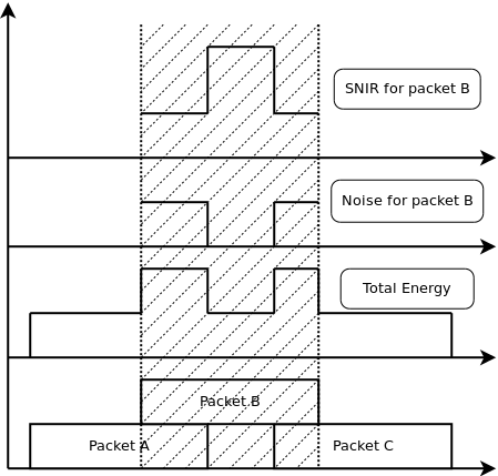
SNIR function over time.
From the SNIR function we can derive bit error rates for BPSK and QAM modulations. Then, for each interval l where BER is constant, we define the upper bound of a probability that an error is present in the chunk of bits located in the interval l for packet k. If we assume an AWGN channel, binary convolutional coding (which is the case in 802.11a) and hard-decision Viterbi decoding, the error rate is thus derived, and the packet error probability for packet k can be computed.
WifiChannel configuration
WifiChannel models include both a PropagationDelayModel and a PropagationLossModel. The following PropagationDelayModels are available:
- ConstantSpeedPropagationDelayModel
- RandomPropagationDelayModel
The following PropagationLossModels are available:
- RandomPropagationLossModel
- FriisPropagationLossModel
- LogDistancePropagationLossModel
- JakesPropagationLossModel
- CompositePropagationLossModel
The MAC model
The 802.11 Distributed Coordination Function is used to calculate when to grant access to the transmission medium. While implementing the DCF would have been particularly easy if we had used a recurring timer that expired every slot, we chose to use the method described in (missing reference here from Yans paper) where the backoff timer duration is lazily calculated whenever needed since it is claimed to have much better performance than the simpler recurring timer solution.
The higher-level MAC functions are implemented in a set of other C++ classes and deal with:
- packet fragmentation and defragmentation,
- use of the rts/cts protocol,
- rate control algorithm,
- connection and disconnection to and from an Access Point,
- the MAC transmission queue,
- beacon generation,
- msdu aggregation,
- etc.
Wifi Attributes
The WifiNetDevice makes heavy use of the ns-3 Attributes subsystem for configuration and default value management. Presently, approximately 100 values are stored in this system.
For instance, class ns-3::WifiMac exports these attributes:
- CtsTimeout: When this timeout expires, the RTS/CTS handshake has failed.
- AckTimeout: When this timeout expires, the DATA/ACK handshake has failed.
- Sifs: The value of the SIFS constant.
- EifsNoDifs: The value of EIFS-DIFS
- Slot: The duration of a Slot.
- Pifs: The value of the PIFS constant.
- MaxPropagationDelay: The maximum propagation delay. Unused for now.
- MaxMsduSize: The maximum size of an MSDU accepted by the MAC layer.This value conforms to the specification.
- Ssid: The ssid we want to belong to.
Wifi Tracing
This needs revised/updating based on the latest Doxygen
ns-3 has a sophisticated tracing infrastructure that allows users to hook into existing trace sources, or to define and export new ones.
Wifi-related trace sources that are available by default include::
* ``ns3::WifiNetDevice``
- Rx: Received payload from the MAC layer.
- Tx: Send payload to the MAC layer.
ns3::WifiPhy
- State: The WifiPhy state
- RxOk: A packet has been received successfully.
- RxError: A packet has been received unsuccessfully.
- Tx: Packet transmission is starting.
Briefly, this means, for example, that a user can hook a processing function to the “State” tracing hook above and be notified whenever the WifiPhy model changes state.
Mesh NetDevice
Placeholder chapter
The Mesh NetDevice based on 802.11s was added in ns-3.6. An overview presentation by Kirill Andreev was published at the wns-3 workshop in 2009: http://www.nsnam.org/wiki/index.php/Wns3-2009.
Bridge NetDevice
Placeholder chapter
Some examples of the use of Bridge NetDevice can be found in examples/csma/ directory.
Wimax NetDevice
This chapter describes the ns-3 WimaxNetDevice and related models. By adding WimaxNetDevice objects to ns-3 nodes, one can create models of 802.16-based networks. Below, we list some more details about what the ns-3 WiMAX models cover but, in summary, the most important features of the ns-3 model are:
- a scalable and realistic physical layer and channel model
- a packet classifier for the IP convergence sublayer
- efficient uplink and downlink schedulers
- support for Multicast and Broadcast Service (MBS), and
- packet tracing functionality
The source code for the WiMAX models lives in the directory src/devices/wimax.
There have been two academic papers published on this model:
- M.A. Ismail, G. Piro, L.A. Grieco, and T. Turletti, “An Improved IEEE 802.16 WiMAX Module for the NS-3 Simulator”, SIMUTools 2010 Conference, March 2010.
- J. Farooq and T. Turletti, “An IEEE 802.16 WiMAX module for the NS-3 Simulator,” SIMUTools 2009 Conference, March 2009.
Scope of the model
From a MAC perspective, there are two basic modes of operation, that of a Subscriber Station (SS) or a Base Station (BS). These are implemented as two subclasses of the base class ns3::NetDevice, class SubscriberStationNetDevice and class BaseStationNetDevice. As is typical in ns-3, there is also a physical layer class WimaxPhy and a channel class WimaxChannel which serves to hold the references to all of the attached Phy devices. The main physical layer class is the SimpleOfdmWimaxChannel class.
Another important aspect of WiMAX is the uplink and downlink scheduler, and there are three primary scheduler types implemented:
- SIMPLE: a simple priority based FCFS scheduler
- RTPS: a real-time polling service (rtPS) scheduler
- MBQOS: a migration-based uplink scheduler
The following additional aspects of the 802.16 specifications, as well as physical layer and channel models, are modelled:
- leverages existing ns-3 wireless propagation loss and delay models, as well as ns-3 mobility models
- Point-to-Multipoint (PMP) mode and the WirelessMAN-OFDM PHY layer
- Initial Ranging
- Service Flow Initialization
- Management Connection
- Transport Initialization
- UGS, rtPS, nrtPS, and BE connections
The following aspects are not presently modelled but would be good topics for future extensions:
- OFDMA PHY layer
- Link adaptation
- Mesh topologies
- ARQ
- ertPS connection
- packet header suppression
Using the Wimax models
The main way that users who write simulation scripts will typically interact with the Wimax models is through the helper API and through the publicly visible attributes of the model.
The helper API is defined in src/helper/wimax-helper.{cc,h}.
The example examples/wimax/wimax-simple.cc contains some basic code that shows how to set up the model::
switch (schedType)
  {
  case 0:
    scheduler = WimaxHelper::SCHED_TYPE_SIMPLE;
    break;
  case 1:
    scheduler = WimaxHelper::SCHED_TYPE_MBQOS;
    break;
  case 2:
    scheduler = WimaxHelper::SCHED_TYPE_RTPS;
    break;
  default:
    scheduler = WimaxHelper::SCHED_TYPE_SIMPLE;
  }

NodeContainer ssNodes;
NodeContainer bsNodes;

ssNodes.Create (2);
bsNodes.Create (1);

WimaxHelper wimax;

NetDeviceContainer ssDevs, bsDevs;

ssDevs = wimax.Install (ssNodes,
                        WimaxHelper::DEVICE_TYPE_SUBSCRIBER_STATION,
                        WimaxHelper::SIMPLE_PHY_TYPE_OFDM,
                        scheduler);
bsDevs = wimax.Install (bsNodes, WimaxHelper::DEVICE_TYPE_BASE_STATION, WimaxHelper::SIMPLE_PHY_TYPE_OFDM, scheduler);
This example shows that there are two subscriber stations and one base station created. The helper method Install allows the user to specify the scheduler type, the physical layer type, and the device type.
Different variants of Install are available; for instance, the example examples/wimax/wimax-multicast.cc shows how to specify a non-default channel or propagation model::
channel = CreateObject<SimpleOfdmWimaxChannel> ();
channel->SetPropagationModel (SimpleOfdmWimaxChannel::COST231_PROPAGATION);
ssDevs = wimax.Install (ssNodes,
                        WimaxHelper::DEVICE_TYPE_SUBSCRIBER_STATION,
                        WimaxHelper::SIMPLE_PHY_TYPE_OFDM,
                        channel,
                        scheduler);
Ptr<WimaxNetDevice> dev = wimax.Install (bsNodes.Get (0),
                                         WimaxHelper::DEVICE_TYPE_BASE_STATION,
                                         WimaxHelper::SIMPLE_PHY_TYPE_OFDM,
                                         channel,
                                         scheduler);
Mobility is also supported in the same way as in Wifi models; see the examples/wimax/wimax-multicast.cc.
Another important concept in WiMAX is that of a service flow. This is a unidirectional flow of packets with a set of QoS parameters such as traffic priority, rate, scheduling type, etc. The base station is responsible for issuing service flow identifiers and mapping them to WiMAX connections. The following code from examples/wimax/wimax-multicast.cc shows how this is configured from a helper level::
ServiceFlow MulticastServiceFlow = wimax.CreateServiceFlow (ServiceFlow::SF_DIRECTION_DOWN,
                                                             ServiceFlow::SF_TYPE_UGS,
                                                             MulticastClassifier);

 bs->GetServiceFlowManager ()->AddMulticastServiceFlow (MulticastServiceFlow, WimaxPhy::MODULATION_TYPE_QPSK_12);
Wimax Attributes
The WimaxNetDevice makes heavy use of the ns-3 Attributes subsystem for configuration and default value management. Presently, approximately 60 values are stored in this system.
For instance, class ns-3::SimpleOfdmWimaxPhy exports these attributes:
- NoiseFigure: Loss (dB) in the Signal-to-Noise-Ratio due to non-idealities in the receiver.
- TxPower: Transmission power (dB)
- G: The ratio of CP time to useful time
- txGain: Transmission gain (dB)
- RxGain: Reception gain (dB)
- Nfft: FFT size
- TraceFilePath: Path to the directory containing SNR to block error rate files
For a full list of attributes in these models, consult the Doxygen page that lists all attributes for ns-3.
Wimax Tracing
ns-3 has a sophisticated tracing infrastructure that allows users to hook into existing trace sources, or to define and export new ones.
Many ns-3 users use the built-in Pcap or Ascii tracing, and the WimaxHelper has similar APIs::
AsciiTraceHelper ascii;
WimaxHelper wimax;
wimax.EnablePcap ("wimax-program", false);
wimax.EnableAsciiAll (ascii.CreateFileStream ("wimax-program.tr");
Unlike other helpers, there is also a special EnableAsciiForConnection() method that limits the ascii tracing to a specific device and connection.
These helpers access the low level trace sources that exist in the WiMAX physical layer, net device, and queue models. Like other ns-3 trace sources, users may hook their own functions to these trace sources if they want to do customized things based on the packet events. See the Doxygen List of trace sources for a complete list of these sources.
Wimax MAC model
The 802.16 model provided in ns-3 attempts to provide an accurate MAC and PHY level implementation of the 802.16 specification with the Point-to-Multipoint (PMP) mode and the WirelessMAN-OFDM PHY layer. The model is mainly composed of three layers:
- The convergence sublayer (CS)
- The MAC CP Common Part Sublayer (MAC-CPS)
- Physical (PHY) layer
The following figure WimaxArchitecture shows the relationships of these models.
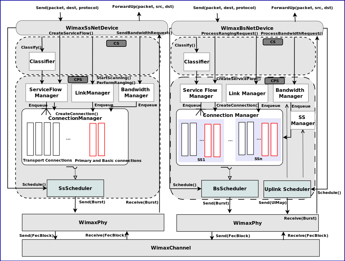
WiMAX architecture.
the Convergence Sublayer ++++++++++++++++++++++++
The Convergence sublayer (CS) provided with this module implements the Packet CS, designed to work with the packet-based protocols at higher layers. The CS is responsible of receiving packet from the higher layer and from peer stations, classifying packets to appropriate connections (or service flows) and processing packets. It keeps a mapping of transport connections to service flows. This enables the MAC CPS identifying the Quality of Service (QoS) parameters associated to a transport connection and ensuring the QoS requirements. The CS currently employs an IP classifier.
IP Packet Classifier ++++++++++++++++++++
An IP packet classifier is used to map incoming packets to appropriate connections based on a set of criteria. The classifier maintains a list of mapping rules which associate an IP flow (src IP address and mask, dst IP address and mask, src port range, dst port range and protocol) to one of the service flows. By analyzing the IP and the TCP/UDP headers the classifier will append the incoming packet (from the upper layer) to the queue of the appropriate WiMAX connection. Class IpcsClassifier and class IpcsClassifierRecord implement the classifier module for both SS and BS
MAC Common Part Sublayer
The MAC Common Part Sublayer (CPS) is the main sublayer of the IEEE 802.16 MAC and performs the fundamental functions of the MAC. The module implements the Point-Multi-Point (PMP) mode. In PMP mode BS is responsible of managing communication among multiple SSs. The key functionalities of the MAC CPS include framing and addressing, generation of MAC management messages, SS initialization and registration, service flow management, bandwidth management and scheduling services. Class WimaxNetDevice represents the MAC layer of a WiMAX network device. This class extends the class NetDevice of the ns-3 API that provides abstraction of a network device. Class WimaxNetDevice is further extended by class BaseStationNetDevice and class SubscriberStationNetDevice, defining MAC layers of BS and SS, respectively. Besides these main classes, the key functions of MAC are distributed to several other classes.
Framing and Management Messages
The module implements a frame as a fixed duration of time, i.e., frame boundaries are defined with respect to time. Each frame is further subdivided into downlink (DL) and uplink (UL) subframes. The module implements the Time Division Duplex (TDD) mode where DL and UL operate on same frequency but are separated in time. A number of DL and UL bursts are then allocated in DL and UL subframes, respectively. Since the standard allows sending and receiving bursts of packets in a given DL or UL burst, the unit of transmission at the MAC layer is a packet burst. The module implements a special PacketBurst data structure for this purpose. A packet burst is essentially a list of packets. The BS downlink and uplink schedulers, implemented by class BSScheduler and class UplinkScheduler, are responsible of generating DL and UL subframes, respectively. In the case of DL, the subframe is simulated by transmitting consecutive bursts (instances PacketBurst). In case of UL, the subframe is divided, with respect to time, into a number of slots. The bursts transmitted by the SSs in these slots are then aligned to slot boundaries. The frame is divided into integer number of symbols and Physical Slots (PS) which helps in managing bandwidth more effectively. The number of symbols per frame depends on the underlying implementation of the PHY layer. The size of a DL or UL burst is specified in units of symbols.
Network Entry and Initialization
The network entry and initialization phase is basically divided into two sub-phases, (1) scanning and synchronization and (2) initial ranging. The entire phase is performed by the LinkManager component of SS and BS. Once an SS wants to join the network, it first scans the downlink frequencies to search for a suitable channel. The search is complete as soon as it detects a PHY frame. The next step is to establish synchronization with the BS. Once SS receives a Downlink-MAP (DL-MAP) message the synchronization phase is complete and it remains synchronized as long as it keeps receiving DL-MAP and Downlink Channel Descriptor (DCD) messages. After the synchronization is established, SS waits for a Uplink Channel Descriptor (UCD) message to acquire uplink channel parameters. Once acquired, the first sub-phase of the network entry and initialization is complete. Once synchronization is achieved, the SS waits for a UL-MAP message to locate a special grant, called initial ranging interval, in the UL subframe. This grant is allocated by the BS Uplink Scheduler at regular intervals. Currently this interval is set to 0.5 ms, however the user is enabled to modify its value from the simulation script.
Connections and Addressing
All communication at the MAC layer is carried in terms of connections. The standard defines a connection as a unidirectional mapping between the SS and BS’s MAC entities for the transmission of traffic. The standard defines two types of connections: management connections for transmitting control messages and transport connections for data transmission. A connection is identified by a 16-bit Connection Identifier (CID). Class WimaxConnection and class Cid implement the connection and CID, respectively. Note that each connection maintains its own transmission queue where packets to transmit on that connection are queued. The ConnectionManager component of BS is responsible of creating and managing connections for all SSs.
The two key management connections defined by the standard, namely the Basic and Primary management connections, are created and allocated to the SS during the ranging process. Basic connection plays an important role throughout the operation of SS also because all (unicast) DL and UL grants are directed towards SS’s Basic CID. In addition to management connections, an SS may have one or more transport connections to send data packets. The Connection Manager component of SS manages the connections associated to SS. As defined by the standard, a management connection is bidirectional, i.e., a pair of downlink and uplink connections is represented by the same CID. This feature is implemented in a way that one connection (in DL direction) is created by the BS and upon receiving the CID the SS then creates an identical connection (in UL direction) with the same CID.
Scheduling Services
The module supports the four scheduling services defined by the 802.16-2004 standard:
- Unsolicited Grant Service (UGS)
- Real-Time Polling Services (rtPS)
- Non Real-Time Polling Services (nrtPS)
- Best Effort (BE)
These scheduling services behave differently with respect to how they request bandwidth as well as how the it is granted. Each service flow is associated to exactly one scheduling service, and the QoS parameter set associated to a service flow actually defines the scheduling service it belongs to. When a service flow is created the UplinkScheduler calculates necessary parameters such as grant size and grant interval based on QoS parameters associated to it.
WiMAX Uplink Scheduler Model
Uplink Scheduler at the BS decides which of the SSs will be assigned uplink allocations based on the QoS parameters associated to a service flow (or scheduling service) and bandwidth requests from the SSs. Uplink scheduler together with Bandwidth Manager implements the complete scheduling service functionality. The standard defines up to four scheduling services (BE, UGS, rtPS, nrtPS) for applications with different types of QoS requirements. The service flows of these scheduling services behave differently with respect to how they request for bandwidth as well as how the bandwidth is granted. The module supports all four scheduling services. Each service flow is associated to exactly one transport connection and one scheduling service. The QoS parameters associated to a service flow actually define the scheduling service it belongs to. Standard QoS parameters for UGS, rtPS, nrtPS and BE services, as specified in Tables 111a to 111d of the 802.16e amendment, are supported. When a service flow is created the uplink scheduler calculates necessary parameters such as grant size and allocation interval based on QoS parameters associated to it. The current WiMAX module provides three different versions of schedulers.
- The first one is a simple priority-based First Come First Serve (FCFS). For the real-time services (UGS and rtPS) the BS then allocates grants/polls on regular basis based on the calculated interval. For the non real-time services (nrtPS and BE) only minimum reserved bandwidth is guaranteed if available after servicing real-time flows. Note that not all of these parameters are utilized by the uplink scheduler. Also note that currently only service flow with fixed-size packet size are supported, as currently set up in simulation scenario with OnOff application of fixed packet size. This scheduler is implemented by class BSSchedulerSimple and class UplinkSchedulerSimple.
- The second one is similar to first scheduler except by rtPS service flow. All rtPS Connections are able to transmit all packet in the queue according to the available bandwidth. The bandwidth saturation control has been implemented to redistribute the effective available bandwidth to all rtPS that have at least one packet to transmit. The remaining bandwidth is allocated to nrtPS and BE Connections. This scheduler is implemented by class BSSchedulerRtps and class UplinkSchedulerRtps.
- The third one is a Migration-based Quality of Service uplink scheduler This uplink scheduler uses three queues, the low priority queue, the intermediate queue and the high priority queue. The scheduler serves the requests in strict priority order from the high priority queue to the low priority queue. The low priority queue stores the bandwidth requests of the BE service flow. The intermediate queue holds bandwidth requests sent by rtPS and by nrtPS connections. rtPS and nrtPS requests can migrate to the high priority queue to guarantee that their QoS requirements are met. Besides the requests migrated from the intermediate queue, the high priority queue stores periodic grants and unicast request opportunities that must be scheduled in the following frame. To guarantee the maximum delay requirement, the BS assigns a deadline to each rtPS bandwidth request in the intermediate queue. The minimum bandwidth requirement of both rtPS and nrtPS connections is guaranteed over a window of duration T. This scheduler is implemented by class UplinkSchedulerMBQoS.
WiMAX Outbound Schedulers Model
Besides the uplink scheduler these are the outbound schedulers at BS and SS side (BSScheduler and SSScheduler). The outbound schedulers decide which of the packets from the outbound queues will be transmitted in a given allocation. The outbound scheduler at the BS schedules the downlink traffic, i.e., packets to be transmitted to the SSs in the downlink subframe. Similarly the outbound scheduler at a SS schedules the packet to be transmitted in the uplink allocation assigned to that SS in the uplink subframe. All three schedulers have been implemented to work as FCFS scheduler, as they allocate grants starting from highest priority scheduling service to the lower priority one (UGS> rtPS> nrtPS> BE). The standard does not suggest any scheduling algorithm and instead leaves this decision up to the manufacturers. Of course more sophisticated algorithms can be added later if required.
WimaxChannel and WimaxPhy models
The module implements the Wireless MAN OFDM PHY specifications as the more relevant for implementation as it is the schema chosen by the WiMAX Forum. This specification is designed for non-light-of-sight (NLOS) including fixed and mobile broadband wireless access. The proposed model uses a 256 FFT processor, with 192 data subcarriers. It supports all the seven modulation and coding schemes specified by Wireless MAN-OFDM. It is composed of two parts: the channel model and the physical model.
Channel model
The channel model we propose is implemented by the class SimpleOFDMWimaxChannel which extends the class wimaxchannel. The channel entity has a private structure named m_phyList which handles all the physical devices connected to it. When a physical device sends a packet (FEC Block) to the channel, the channel handles the packet, and then for each physical device connected to it, it calculates the propagation delay, the path loss according to a given propagation model and eventually forwards the packet to the receiver device. The channel class uses the method GetDistanceFrom() to calculate the distance between two physical entities according to their 3D coordinates. The delay is computed as delay = distance/C, where C is the speed of the light.
Physical model
The physical layer performs two main operations: (i) It receives a burst from a channel and forwards it to the MAC layer, (ii) it receives a burst from the MAC layer and transmits it on the channel. In order to reduce the simulation complexity of the WiMAX physical layer, we have chosen to model offline part of the physical layer. More specifically we have developed an OFDM simulator to generate trace files used by the reception process to evaluate if a FEC block can be correctly decoded or not.
Transmission Process: A burst is a set of WiMAX MAC PDUs. At the sending process, a burst is converted into bit-streams and then splitted into smaller FEC blocks which are then sent to the channel with a power equal P_tx.
Reception Process: The reception process includes the following operations:
- Receive a FEC block from the channel.
- Calculate the noise level.
- Estimate the signal to noise ratio (SNR) with the following formula.
- Determine if a FEC block can be correctly decoded.
- Concatenate received FEC blocks to reconstruct the original burst.
- Forward the burst to the upper layer.
The developed process to evaluate if a FEC block can be correctly received or not uses pre-generated traces. The trace files are generated by an external OFDM simulator (described later). A class named SNRToBlockErrorRateManager handles a repository containing seven trace files (one for each modulation and coding scheme). A repository is specific for a particular channel model.
A trace file is made of 6 columns. The first column provides the SNR value (1), whereas the other columns give respectively the bit error rate BER (2), the block error rate BlcER(3), the standard deviation on BlcER, and the confidence interval (4 and 5). These trace files are loaded into memory by the SNRToBlockErrorRateManager entity at the beginning of the simulation.
Currently, The first process uses the first and third columns to determine if a FEC block is correctly received. When the physical layer receives a packet with an SNR equal to SNR_rx, it asks the SNRToBlockErrorRateManager to return the corresponding block error rate BlcER. A random number RAND between 0 and 1 is then generated. If RAND is greater than BlcER, then the block is correctly received, otherwise the block is considered erroneous and is ignored.
The module provides defaults SNR to block error rate traces in default-traces.h. The traces have been generated by an External WiMAX OFDM simulator. The simulator is based on an external mathematics and signal processing library IT++ and includes : a random block generator, a Reed Solomon (RS) coder, a convolutional coder, an interleaver, a 256 FFT-based OFDM modulator, a multi-path channel simulator and an equalizer. The multipath channel is simulated using the TDL_channel class of the IT++ library.
Users can configure the module to use their own traces generated by another OFDM simulator or ideally by performing experiments in real environment. For this purpose, a path to a repository containing trace files should be provided. If no repository is provided the traces form default-traces.h will be loaded. A valid repository should contain 7 files, one for each modulation and coding scheme.
The names of the files should respect the following format: modulation0.txt for modulation 0, modulation1.txt for modulation 1 and so on... The file format should be as follows:
SNR_value1   BER  Blc_ER  STANDARD_DEVIATION  CONFIDENCE_INTERVAL1  CONFIDENCE_INTERVAL2
SNR_value2   BER  Blc_ER  STANDARD_DEVIATION  CONFIDENCE_INTERVAL1  CONFIDENCE_INTERVAL2
 ...          ...  ...     ...                 ...                   ...
 ...          ...  ...     ...                 ...                   ...
LTE Module
This chapter describes the ns-3 ns3::LteNetDevice and related models. By adding ns3::LteNetDevice objects to ns-3 nodes, one can create models of 3GPP E-UTRAN infrastructure and Long Term Evolution (LTE) networks.
Below, we list some more details about what ns-3 LTE models cover but, in summary, the most important features of the ns-3 model are:
- a basic implementation of both the User Equipment (UE) and the enhanced NodeB (eNB) devices,
- RRC entities for both the UE and the eNB,
- a state-of-the-art Adaptive Modulation and Coding (AMC) scheme for the downlink
- the management of the data radio bearers (with their QoS parameters), the MAC queues and the RLC instances,
- Channel Quality Indicator (CQI) management,
- support for both uplink and downlik packet scheduling,
- a PHY layer model with Resource Block level granularity
- a channel model with the outdoor E-UTRAN propagation loss model.
Model Description
The source code for the LTE models lives in the directory src/devices/lte.
Design
The LTE model provides a basic implementation of LTE devices, including propagation models and PHY and MAC layers. It allow to simulate an E-UTRAN interface where one eNB and several UEs can communicate among them using a shared downlink (uplink) channel.
The PHY layer has been developed extending the Spectrum Framework [1]. The MAC model, instead, has been developed extending and adding some features to the base class ns3::NetDevice.
Physical layer
A ns3::LtePhy class models the LTE PHY layer.
Basic functionalities of the PHY layer are: (i) transmit packets coming from the device to the channel; (ii) receive packets from the channel; (ii) evaluate the quality of the channel from the Signal To Noise ratio of the received signal; and (iii) forward received packets to the device.
Both the PHY and channel have been developed extending ns3::SpectrumPhy and ns3::SpectrumChannel classes, respectively.
The module implements an FDD channel access. In FDD channel access, downlink and uplink transmissions work together in the time but using a different set of frequencies. Since DL and UL are indipendent between them, the PHY is composed by couple of ns3::LteSpectrumPhy object (i.e., implemented into the ns3::LteSpectrumPhy class); one for the downlink and one for the uplink. The ns3::LtePhy stores and manages both downlink and uplink ns3::LteSpectrumPhy elements.
In order to customize all physical functionalities for both UE and eNB devices, dedicated classes have been inherited from ones described before. In particular, ns3::UePhy and ns3::EnbPhy classes, inherited from the ns3::LtePhy class, implement the PHY layer for the UE and the eNB, respectively. In the same way, ns3::UeLteSpectrumPhy and ns3::EnbLteSpectrumPhy classes, inherited from the ns3::LteSpectrumPhy, implement the downlink/uplink spectrum channel for the UE and the eNB, respectively.
The figure below shows how UE and eNB can exchange packets through the considered PHY layer.
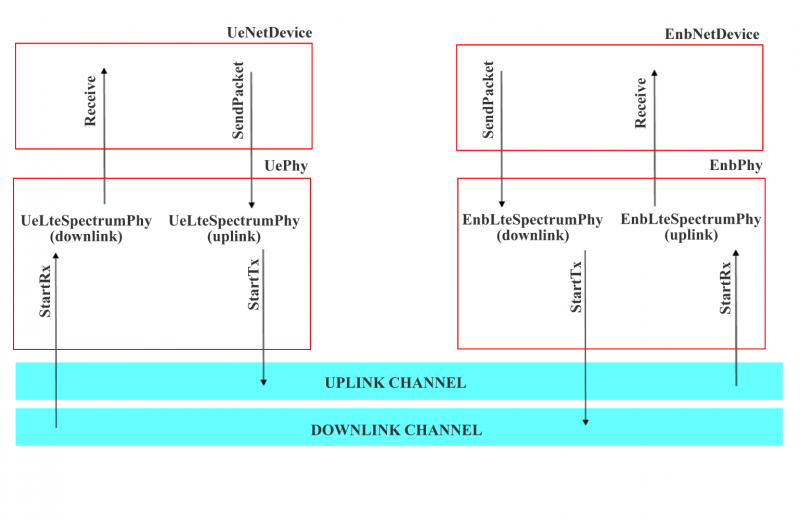
DL and UL transmision on the LTE network
For the downlink, when the eNB whants to send packets, it calls the StartTx function to send them into the downlink channel. Then, the downlink channel delivers the burst of packets to all the ns3::UeLteSpectrumPhy attached to it, handling the StartRx function. When the UE receives packets, it executes the following tasks:
- compute the SINR for all the sub channel used in the downlink
- create and send CQI feedbacks
- forward all the received packets to the device
The uplink works similary to the previous one.
Propagation Loss Models
A proper propagation loss model has been developed for the LTE E-UTRAN interface (see [2] and [3]). It is used by the PHY layer to compute the loss due to the propagation.
The LTE propagation loss model is composed by 4 different models (shadowing, multipath, penetration loss and path loss) [2]:
- Pathloss:
 , where R is the distance between the
UE and the eNB in Km.
, where R is the distance between the
UE and the eNB in Km. - Multipath: Jakes model
- PenetrationLoss: 10 dB
- Shadowing: log-normal distribution (mean=0dB, standard deviation=8dB)
Every time that the LteSpectrumPHY::StartRx () function is called, the SpectrumInterferenceModel is used to computed the SINR, as proposed in [3]. Then, the network device uses the AMC module to map the SINR to a proper CQI and to send it to the eNB using the ideal control channel.
LTE Devices
All the common functionalities of the LTE network devices have been defined into the ns3::LteNetDevice class. Moreover, the LTE device has been conceived as a container of several entities such as MAC, RRC, RLC etc .. For each of these entity a dedicated class has been developed.
For each device are defined the following entity/element
- the LTE PHY layer (described in the previous sub section)
- rrc entity
- mac entity
- rlc entity
The module is perfectly integrated into the whole ns-3 project: it is already possible to attach to each device a TCP/IP protocol stack and all the implemented applications (i.e., udp client/server, trace based, etc..).
The RRC Entity
RRC entity is implemented by the ns3::RrcEntity class, and provides only the Radio Bearer management functionality. A dedicated bearer is created for each downlink flow.
The RRC entity performs the classification of the packets coming from the upper layer into the corresponding Radio Bearer. This classification is based on the information provided by the class ns3::IpcsClassifierRecord.
The MAC Entity
Class ns3::MacEntity provides a basic implementation of the MAC entity for the LTE device. Moreover, ns3::EnbMacEntity and ns3::UeMacEntity classes, inherited from the previous one, provides an implementation for the eNB and the UE MAC entity, respectively. In all MAC entities is defined the AMC module [4]_. Furthermore, into the :cpp:class:`ns3::EnbMacEntity class are defined also both uplink and downlink schedulers.
Every time the PHY layer of the UE receives a packet form the channel, it calls the AMC module, define into the MAC entity, in order to convert the SINR of the received signal to CQI feedbacks. Every sub frame, the eNB performs both uplink and downlink radio resource allocation. Actually only a simple packet scheduler has been implemented that is able to send, every sub frame, only one packet in the downlink.
The RLC Entity
The RLC entity performs an interface between the MAC layer and the MAC queue for a given bearer. Actually, only the RLC Transport Mode has been implemented.
Control Channel
Control channel keeps a very important role in LTE networks. In fact, it is responsible of the transmission of several information (i.e., CQI feedback, allocation map, etc...). For this reason, also in a framework oriented to data transmision, it is necesary to find a tecnique for exchange these information. To this aim, an ideal control channel will be developed. Using ideal control messages, both UE and eNB can exchange control information without simulating a realistic transmission over the LTE channel.
Two types of control messages have been implemented: the Pdcch Map Ideal Control Message and the Cqi Ideal Control Message. The first one is used by the eNB to send the uplink and downlink resource mapping to all registered UE. In particular, this message carries information about UEs that have been scheduled in the ul/dl, a list of assigned sub channels and the selected MCS for the transmission. The second one, instead, is used by the UE to send CQI feedbacks to the eNB.
Scope and Limitations
The framework has been designed in order to support data transmission for both uplink and downlink. It is important to note that downlin and uplink transmissions are managed by the packet scheduler that works at the eNB. It decides, in fact, what UEs should be scheduled every TTI and what radio resource should be allocated to them.
In the current implementation, the downlink transmission is administrated by the downlink packet scheduler. Furthermore, no packet scheduler for uplink transmission has been developed. As a consequence, for the downlink packet are sent only after scheduling decisions; for the uplink, instead, packet are sent directly, without any scheduling decisions.
Finally, the transmission of control messages (such as CQI feedbacks, PDCCH, etc..) is done by an ideal control channel.
Future Work
In the future, several LTE features will be developed in order to improve the proposed module.
In particular, for the near future have been scheduled the following implementations:
- a more efficient design for the RRM (Radio resource management)
- a complete packet scheduler (i.e., a simple round robin scheme, maximum througput and proportional fair allocation schemes) for both downlink and uplink, in order to support a standard compliant packet transmission
- ideal PDCCH control messages
- a standard compliant RLC entity
- PHY error model
References
| [1] | N. Baldo and M. Miozzo, Spectrum-aware Channel and PHY layer modeling for ns3, Proceedings of ICST NSTools 2009, Pisa, Italy. The framework is designed to simulate only data transmissions. For the transmission of control messages (such as CQI feedback, PDCCH, etc..) will be used an ideal control channel). |
| [2] | (1, 2) 3GPP TS 25.814 ( http://www.3gpp.org/ftp/specs/html-INFO/25814.htm ) |
| [3] | (1, 2) Giuseppe Piro, Luigi Alfredo Grieco, Gennaro Boggia, and Pietro Camarda”, A Two-level Scheduling Algorithm for QoS Support in the Downlink of LTE Cellular Networks”, Proc. of European Wireless, EW2010, Lucca, Italy, Apr., 2010 ( draft version is available on http://telematics.poliba.it/index.php?option=com_jombib&task=showbib&id=330 ) |
| [4] | 3GPP R1-081483 (available on http://www.3gpp.org/ftp/tsg_ran/WG1_RL1/TSGR1_52b/Docs/R1-081483.zip ) |
Usage
The main way that users who write simulation scripts will typically interact with the LTE models is through the helper API and through the publicly visible attributes of the model.
The helper API is defined in src/devices/lte/helper/lte-helper.h.
The example src/devices/lte/examples/ contain some basic code that shows how to set up the model in order to simualte an E-UTRAN downlink transmission.
Examples
src/devices/lte/examples/lte-device.cc shows how it is possible to set up the LTE module:
NodeContainer ueNodes;
NodeContainer enbNodes;

ueNodes.Create (1);
enbNodes.Create (1);

LteHelper lte;

NetDeviceContainer ueDevs, enbDevs;
ueDevs = lte.Install (ueNodes, LteHelper::DEVICE_TYPE_USER_EQUIPMENT);
enbDevs = lte.Install (enbNodes, LteHelper::DEVICE_TYPE_ENODEB);
The helper method ns3::LteHelper::Install() creates LTE device, the DL, UL physical layer and attach the to proper LTE channels.
Moreover, to simulate a complete LTE system, it is necessary to define other information, as expressed in what follows:
install IP protocol stack:
InternetStackHelper stack;
stack.Install (ueNodes);
stack.Install (enbNodes);
Ipv4AddressHelper address;
address.SetBase ("10.1.1.0", "255.255.255.0");
Ipv4InterfaceContainer UEinterfaces = address.Assign (ueDevs);
Ipv4InterfaceContainer ENBinterface = address.Assign (enbDevs);
register UE to a given eNB:
Ptr<EnbNetDevice> enb = enbDevs.Get (0)->GetObject<EnbNetDevice> ();
Ptr<UeNetDevice> ue = ueDevs.Get (i)->GetObject<UeNetDevice> ();
lte.RegisterUeToTheEnb (ue, enb);
create the mobility model for each device:
Ptr<ConstantPositionMobilityModel> enbMobility = new ConstantPositionMobilityModel ();
enbMobility->SetPosition (Vector (0.0, 0.0, 0.0));
lte.AddMobility (enb->GetPhy (), enbMobility);

Ptr<ConstantVelocityMobilityModel> ueMobility = new ConstantVelocityMobilityModel ();
ueMobility->SetPosition (Vector (30.0, 0.0, 0.0));
ueMobility->SetVelocity (Vector (30.0, 0.0, 0.0));
lte.AddMobility (ue->GetPhy (), ueMobility);
define a set of sub channels to use for dl and ul transmission:
std::vector<int> dlSubChannels;
for (int i = 0; i < 25; i++)
  {
    dlSubChannels.push_back (i);
  }
std::vector<int> ulSubChannels;
for (int i = 50; i < 100; i++)
  {
    ulSubChannels.push_back (i);
  }

enb->GetPhy ()->SetDownlinkSubChannels (dlSubChannels);
enb->GetPhy ()->SetUplinkSubChannels (ulSubChannels);
ue->GetPhy ()->SetDownlinkSubChannels (dlSubChannels);
ue->GetPhy ()->SetUplinkSubChannels (ulSubChannels);
define a channel realization for the PHY model:
lte.AddDownlinkChannelRealization (enbMobility, ueMobility, ue->GetPhy ());
Helpers
Attributes
Tracing
Logging
Caveats
Validation
In the src/devices/lte/example/lte-amc.cc has been developed an important example that shows the proper functioning of both AMC module and Channel model. The analyzed scenario is composed by two nodes: a eNB and a single UE (registered to the eNB). The UE moves into the cell using the ns3::ConstantVelocityMobilityModel, along a radial direction. The proposed example describes how the channel quality decreases as the distance between UE and eNB increases. As a conseguence, the total bit rate (in bits per TTI) available to the UE decreases as the distance between nodes increases, as expected.
UAN Framework
Underwater Acoustics Networks is a research field that, in the last year, is gathering attention from researchers all over the world. In fact, the need for underwater wireless communications exists in applications such as remote control in offshore oil industry [1], pollution monitoring in environmental systems, speech transmission between divers, mapping of the ocean floor, mine counter measures [4], seismic monitoring of ocean faults as well as climate changes monitoring. Unfortunately, making on-field measurements is very expensive and there are no commonly accepted standard to base on. Hence, the priority to make research work going on, it is to realize a complete simulation framework that researchers can use to experiment, make tests and make performance evaluation and comparison.
The NS-3 UAN module is a first step in this direction, trying to offer a reliable and realistic tool. In fact, the UAN module offers accurate modelling of the underwater acoustic channel, a model of the WHOI acoustic modem (one of the widely used acoustic modems)[6]_ and its communications performance, and some MAC protocols.
This project integrates the efforts of UAN module, extending it to make a simulation framework that researchers will be able to use for their aims. The extension consists of an Autonomous Underwater Vehicle (AUV) simulator (navigation and movement) along with an implementation of AUV batteries. Moreover, it will be implemented, a power model for a generic acoustic modem and, the physicals layers will be modified to use such model. For the moment, the UAN module can be used to make some sort of performance comparisons of the available MAC protocols, or tests the communication channel. With this extension, researchers will be able to use the framework to develop and evaluate their “applications”. An application, is intended as a more complete concept, including each parts of the UAN module integrated with the framework’s extensions. Then, the final result is a complete simulation stack for underwater network applications.
Model Description
The source code for the UAN Framework lives in the directory src/devices/uan, src/devices/uan/auv and in src/contrib/energy for the contribution on the li-ion battery model.
The UAN Framework is composed of two main parts:
- the AUV mobility models, including Electric motor propelled AUV (REMUS class [3] [4] ) and Seaglider [5] models
- the energy models, including AUV energy models, AUV energy sources (batteries) and an acoustic modem energy model
As enabling component for the energy models, a Li-Ion batteries energy source has been implemented basing on [7] [8].
Design
The development of the UAN Framework for ns-3 is composed by three consecutive steps. The first one is the development of the AUV simulator, the second one is the development of the UAN energy models and the third one is the integration of such components with the existing modules, UAN module and Energy Model. The module is implemented into the /src/contrib/uan folder for the part regarding acoustic modem energy model and in /src/contrib/uan/auv for the part regarding the AUV simulator.
AUV mobility models
The AUV mobility models have been designed as in the follows.
The user will be able to:
- program the AUV to navigate over a path of waypoints
- control the velocity of the AUV
- control the depth of the AUV
- control the direction of the AUV
- control the pitch of the AUV
- tell the AUV to emerge or submerge to a specified depth
Implement a model of the navigation of AUV. This involves implementing two classes modelling the two major categories of AUVs: electric motor propelled (like REMUS class [3] [4]) and “sea gliders” [5]. The classic AUVs are submarine-like devices, propelled by an electric motor linked with a propeller. Instead, the “sea glider” class exploits small changes in its buoyancy that, in conjunction with wings, can convert vertical motion to horizontal. So, a glider will reach a point into the water by describing a “saw-tooth” movement. Modelling the AUV navigation, involves in considering a real-world AUV class thus, taking into account maximum speed, directional capabilities, emerging and submerging times. Regarding the sea gliders, it is modelled the characteristic saw-tooth movement, with AUV’s speed driven by buoyancy and glide angle.
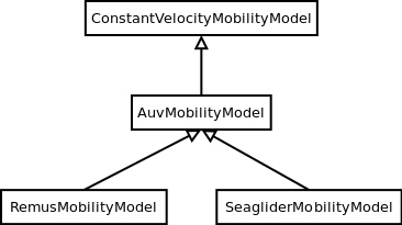
AUV’s mobility model classes overview
An ns3::AuvMobilityModel interface has been designed to give users a generic interface to access AUV’s navigation functions. The AuvMobilityModel interface is implemented by the RemusMobilityModel and the GliderMobilityModel classes. The AUV’s mobility models organization it is shown in AUV’s mobility model classes overview. Both models use a constant velocity movement, thus the AuvMobilityModel interface derives from the ConstantVelocityMobilityModel. The two classes hold the navigation parameters for the two different AUVs, like maximum pitch angles, maximum operating depth, maximum and minimum speed values. The Glider model holds also some extra parameters like maximum buoyancy values, and maximum and minimum glide slopes. Both classes, RemusMobilityModel and GliderMobilityModel, handle also the AUV power consumption, utilizing the relative power models. Has been modified the WaypointMobilityModel to let it use a generic underlying ConstantVelocityModel to validate the waypoints and, to keep trace of the node’s position. The default model is the classic ConstantVelocityModel but, for example in case of REMUS mobility model, the user can install the AUV mobility model into the waypoint model and then validating the waypoints against REMUS navigation constraints.
Energy models
The energy models have been designed as in the follows.
The user will be able to:
- use a specific power profile for the acoustic modem
- use a specific energy model for the AUV
- trace the power consumption of AUV navigation, through AUV’s energy model
- trace the power consumprion underwater acoustic communications, through acoustic modem power profile
We have integrated the Energy Model with the UAN module, to implement energy handling. We have implemented a specific energy model for the two AUV classes and, an energy source for Lithium batteries. This will be really useful for researchers to keep trace of the AUV operational life. We have implemented also an acoustic modem power profile, to keep trace of its power consumption. This can be used to compare protocols specific power performance. In order to use such power profile, the acoustic transducer physical layer has been modified to use the modem power profile. We have decoupled the physical layer from the transducer specific energy model, to let the users change the different energy models without changing the physical layer.
Basing on the Device Energy Model interface, it has been implemented a specific energy model for the two AUV classes (REMUS and Seaglider). This models reproduce the AUV’s specific power consumption to give users accurate information. This model can be naturally used to evaluates the AUV operating life, as well as mission-related power consumption, etc. Have been developed two AUV energy models:
- GliderEnergyModel, computes the power consumption of the vehicle based on the current buoyancy value and vertical speed [5]
- RemusEnergyModel, computes the power consumption of the vehicle based on the current speed, as it is propelled by a brush-less electric motor
Note
TODO extend a little bit
Note
[TODO]
Basing on the Device Energy Model interface, has been implemented a generic energy model for acoustic modem. The model allows to trace four modem’s power-states: Sleep, Idle, Receiving, Transmitting. The default parameters for the energy model are set to fit those of the WHOI μmodem. The class follows pretty closely the RadioEnergyModel class as the transducer behaviour is pretty close to that of a wifi radio.
The default power consumption values implemented into the model are as follows [6]:
| Modem State | Power Consumption |
| TX | 50 W |
| RX | 158 mW |
| Idle | 158 mW |
| Sleep | 5.8 mW |
The UAN module has been modified in order to utilize the implemented energy classes. Specifically, it has been modified the physical layer of the UAN module. It Has been implemented an UpdatePowerConsumption method that takes the modem’s state as parameter. It checks if an energy source is installed into the node and, in case, it then use the AcousticModemEnergyModel to update the power consumption with the current modem’s state. The modem power consumption’s update takes place whenever the modem changes its state.
A user should take into account that, if the the power consumption handling is enabled (if the node has an energy source installed), all the communications processes will terminate whether the node depletes all the energy source.
A generic Li-Ion battery model has been implemented based on [7][8]. The model can be fitted to any type of Li-Ion battery simply changing the model’s parameters The default values are fitted for the Panasonic CGR18650DA Li-Ion Battery [9]. [TODO insert figure] As shown in figure the model approximates very well the Li-Ion cells. Regarding Seagliders, the batteries used into the AUV are Electrochem 3B36 Lithium / Sulfuryl Chloride cells [10]. Also with this cell type, the model seems to approximates the different discharge curves pretty well, as shown in the figure.
Note
should I insert the li-ion model deatils here? I think it is better to put them into an Energy-related chapter..
Scope and Limitations
The framework is designed to simulate AUV’s behaviour. We have modeled the navigation and power consumption behaviour of REMUS class and Seaglider AUVs. The communications stack, associated with the AUV, can be modified depending on simulation needs. Usually, the default underwater stack is being used, composed of an half duplex acoustic modem, an Aloha MAC protocol and a generic physical layer.
Regarding the AUV energy consumption, the user should be aware that the level of accuracy differs for the two classes:
- Seaglider, high level of accuracy, thanks to the availability of detailed information on AUV’s components and behaviour [5] [10]. Have been modeled both the navigation power consumption and the Li battery packs (according to [5]).
- REMUS, medium level of accuracy, due to the lack of publicly available information on AUV’s components. We have approximated the power consumption of the AUV’s motor with a linear behaviour and, the energy source uses an ideal model (BasicEnergySource) with a power capacity equal to that specified in [4].
Future Work
Some ideas could be :
- insert a data logging capability
- modify the framework to use sockets (enabling the possibility to use applications)
- introduce some more MAC protocols
- modify the physical layer to let it consider the doppler spread (problematic in underwater environments)
- introduce OFDM modulations
References
| [1] | BINGHAM, D.; DRAKE, T.; HILL, A.; LOTT, R.; The Application of Autonomous Underwater Vehicle (AUV) Technology in the Oil Industry – Vision and Experiences, URL: http://www.fig.net/pub/fig_2002/Ts4-4/TS4_4_bingham_etal.pdf |
| [2] | AUVfest2008: Underwater mines; URL: http://oceanexplorer.noaa.gov/explorations/08auvfest/background/mines/mines.html |
| [3] | (1, 2) Hydroinc Products; URL: http://www.hydroidinc.com/products.html |
| [4] | (1, 2, 3) WHOI, Autonomous Underwater Vehicle, REMUS; URL: http://www.whoi.edu/page.do?pid=29856 |
| [5] | (1, 2, 3) Eriksen, C.C., T.J. Osse, R.D. Light, T. Wen, T.W. Lehman, P.L. Sabin, J.W. Ballard, and A.M. Chiodi. Seaglider: A Long-Range Autonomous Underwater Vehicle for Oceanographic Research, IEEE Journal of Oceanic Engineering, 26, 4, October 2001. URL: http://ieeexplore.ieee.org/stamp/stamp.jsp?tp=&arnumber=972073&userType=inst |
| [6] | L. Freitag, M. Grund, I. Singh, J. Partan, P. Koski, K. Ball, and W. Hole, The whoi micro-modem: an acoustic communications and navigation system for multiple platforms, In Proc. IEEE OCEANS05 Conf, 2005. URL: http://ieeexplore.ieee.org/iel5/10918/34367/01639901.pdf |
| [7] | C. M. Shepherd, “Design of Primary and Secondary Cells - Part 3. Battery discharge equation,” U.S. Naval Research Laboratory, 1963 |
| [8] | Tremblay, O.; Dessaint, L.-A.; Dekkiche, A.-I., “A Generic Battery Model for the Dynamic Simulation of Hybrid Electric Vehicles,” Ecole de Technologie Superieure, Universite du Quebec, 2007 URL: http://ieeexplore.ieee.org/stamp/stamp.jsp?tp=&arnumber=4544139 |
| [9] | Panasonic CGR18650DA Datasheet, URL: http://www.panasonic.com/industrial/includes/pdf/Panasonic_LiIon_CGR18650DA.pdf |
| [10] | Electrochem 3B36 Datasheet, URL: http://www.electrochem.com.cn/products/Primary/HighRate/CSC/3B36.pdf |
Usage
The main way that users who write simulation scripts will typically interact with the UAN Framework is through the helper API and through the publicly visible attributes of the model.
The helper API is defined in src/devices/uan/helper/acoustic-modem-energy-model-helper.{cc,h} and in /src/devices/uan/auv/helper/...{cc,h}.
The example folder src/devices/uan/auv/examples/ contain some basic code that shows how to set up and use the models. further examples can be found into the Unit tests in src/devices/uan/auv/test/...cc
Examples
Examples of the Framework’s usage can be found into the examples folder. There are mobility related examples and uan related ones.
Mobility Model Examples
- auv-energy-model:
In this example we show the basic usage of an AUV energy model. Specifically, we show how to create a generic node, adding to it a basic energy source and consuming energy from the energy source. In this example we show the basic usage of an AUV energy model.
The Seaglider AUV power consumption depends on buoyancy and vertical speed values, so we simulate a 20 seconds movement at 0.3 m/s of vertical speed and 138g of buoyancy. Then a 20 seconds movement at 0.2 m/s of vertical speed and 138g of buoyancy and then a stop of 5 seconds.
The required energy will be drained by the model basing on the given buoyancy/speed values, from the energy source installed onto the node. We finally register a callback to the TotalEnergyConsumption traced value.
- auv-mobility:
In this example we show how to use the AuvMobilityHelper to install an AUV mobility model into a (set of) node. Then we make the AUV to submerge to a depth of 1000 meters. We then set a callback function called on reaching of the target depth. The callback then makes the AUV to emerge to water surface (0 meters). We set also a callback function called on reaching of the target depth. The emerge callback then, stops the AUV.
During the whole navigation process, the AUV’s position is tracked by the TracePos function and plotted into a Gnuplot graph.
- waypoint-mobility:
We show how to use the WaypointMobilityModel with a non-standard ConstantVelocityMobilityModel. We first create a waypoint model with an underlying RemusMobilityModel setting the mobility trace with two waypoints. We then create a waypoint model with an underlying GliderMobilityModel setting the waypoints separately with the AddWaypoint method. The AUV’s position is printed out every seconds.
UAN Examples
- li-ion-energy-source
In this simple example, we show how to create and drain energy from a LiIonEnergySource. We make a series of discharge calls to the energy source class, with different current drain and durations, until all the energy is depleted from the cell (i.e. the voltage of the cell goes below the threshold level). Every 20 seconds we print out the actual cell voltage to verify that it follows the discharge curve [9]. At the end of the example it is verified that after the energy depletion call, the cell voltage is below the threshold voltage.
- uan-energy-auv
This is a comprehensive example where all the project’s components are used. We setup two nodes, one fixed surface gateway equipped with an acoustic modem and a moving Seaglider AUV with an acoustic modem too. Using the waypoint mobility model with an underlying GliderMobilityModel, we make the glider descend to -1000 meters and then emerge to the water surface. The AUV sends a generic 17-bytes packet every 10 seconds during the navigation process. The gateway receives the packets and stores the total bytes amount. At the end of the simulation are shown the energy consumptions of the two nodes and the networking stats.
Helpers
In this section we give an overview of the available helpers and their behaviour.
AcousticModemEnergyModelHelper
This helper installs AcousticModemEnergyModel into UanNetDevice objects only. It requires an UanNetDevice and an EnergySource as input objects.
The helper creates an AcousticModemEnergyModel with default parameters and associate it with the given energy source. It configures an EnergyModelCallback and an EnergyDepletionCallback. The depletion callback can be configured as a parameter.
AuvGliderHelper
Installs into a node (or set of nodes) the Seaglider’s features:
- waypoint model with underlying glider mobility model
- glider energy model
- glider energy source
- micro modem energy model
The glider mobility model is the GliderMobilityModel with default parameters. The glider energy model is the GliderEnergyModel with default parameters.
Regarding the energy source, the Seaglider features two battery packs, one for motor power and one for digital-analog power. Each pack is composed of 12 (10V) and 42 (24V) lithium chloride DD-cell batteries, respectively [5]. The total power capacity is around 17.5 MJ (3.9 MJ + 13.6 MJ). In the original version of the Seaglider there was 18 + 63 D-cell with a total power capacity of 10MJ.
The packs design is as follows:
- 10V - 3 in-series string x 4 strings = 12 cells - typical capacity ~100 Ah
- 24V - 7 in-series-strings x 6 strings = 42 cells - typical capacity ~150 Ah
Battery cells are Electrochem 3B36, with 3.6 V nominal voltage and 30.0 Ah nominal capacity. The 10V battery pack is associated with the electronic devices, while the 24V one is associated with the pump motor.
The micro modem energy model is the MicroModemEnergyModel with default parameters.
AuvRemusHelper
Install into a node (or set of nodes) the REMUS features:
- waypoint model with REMUS mobility model validation
- REMUS energy model
- REMUS energy source
- micro modem energy model
The REMUS mobility model is the RemusMobilityModel with default parameters. The REMUS energy model is the RemusEnergyModel with default parameters.
Regarding the energy source, the REMUS features a rechargeable lithium ion battery pack rated 1.1 kWh @ 27 V (40 Ah) in operating conditions (specifications from [3] and Hydroinc European salesman). Since more detailed information about battery pack were not publicly available, the energy source used is a BasicEnergySource.
The micro modem energy model is the MicroModemEnergyModel with default parameters.
Attributes
Note
TODO
Tracing
Note
TODO
Logging
Note
TODO
Caveats
Note
TODO
Validation
This model has been tested with three UNIT test:
- auv-energy-model
- auv-mobility
- li-ion-energy-source
Auv Energy Model
Includes test cases for single packet energy consumption, energy depletion, Glider and REMUS energy consumption. The unit test can be found in src/devices/uan/auv/test/auv-energy-model-test.cc.
The single packet energy consumption test do the following:
- creates a two node network, one surface gateway and one fixed node at -500 m of depth
- install the acoustic communication stack with energy consuption support into the nodes
- a packet is sent from the underwater node to the gateway
- it is verified that both, the gateway and the fixed node, have consumed the expected amount of energy from their sources
The energy depletion test do the following steps:
- create a node with an empty energy source
- try to send a packet
- verify that the energy depletion callback has been invoked
The Glider energy consumption test do the following:
- create a node with glider capabilities
- make the vehicle to move to a predetermined waypoint
- verify that the energy consumed for the navigation is correct, according to the glider specifications
The REMUS energy consumption test do the following:
- create a node with REMUS capabilities
- make the vehicle to move to a predetermined waypoint
- verify that the energy consumed for the navigation is correct, according to the REMUS specifications
Auv Mobility
Includes test cases for glider and REMUS mobility models. The unit test can be found in src/devices/uan/auv/test/auv-mobility-test.cc.
- create a node with glider capabilities
- set a specified velocity vector and verify if the resulting buoyancy is the one that is supposed to be
- make the vehicle to submerge to a specified depth and verify if, at the end of the process the position is the one that is supposed to be
- make the vehicle to emerge to a specified depth and verify if, at the end of the process the position is the one that is supposed to be
- make the vehicle to navigate to a specified point, using direction, pitch and speed settings and, verify if at the end of the process the position is the one that is supposed to be
- make the vehicle to navigate to a specified point, using a velocity vector and, verify if at the end of the process the position is the one that is supposed to be
The REMUS mobility model test do the following: * create a node with glider capabilities * make the vehicle to submerge to a specified depth and verify if, at the end of the process the position is the one that is supposed to be * make the vehicle to emerge to a specified depth and verify if, at the end of the process the position is the one that is supposed to be * make the vehicle to navigate to a specified point, using direction, pitch and speed settings and, verify if at the end of the process the position is the one that is supposed to be * make the vehicle to navigate to a specified point, using a velocity vector and, verify if at the end of the process the position is the one that is supposed to be
Li-Ion Energy Source
Includes test case for Li-Ion energy source. The unit test can be found in src/contrib/energy/test/li-ion-energy-source-test.cc.
The test case verify that after a well-known discharge time with constant current drain, the cell voltage has followed the datasheet discharge curve [9].
Energy Framework
Energy consumption is a key issue for wireless devices, and wireless network researchers often need to investigate the energy consumption at a node or in the overall network while running network simulations in ns-3. This requires ns-3 to support energy consumption modeling. Further, as concepts such as fuel cells and energy scavenging are becoming viable for low power wireless devices, incorporating the effect of these emerging technologies into simulations requires support for modeling diverse energy sources in ns-3. The ns-3 Energy Framework provides the basis for energy consumption and energy source modeling.
Model Description
The source code for the Energy Framework is currently at: src/contrib/energy.
Design
The ns-3 Energy Framework is composed of 2 parts: Energy Source and Device Energy Model. The framework will be implemented into the src/contrib/energy/models folder.
Energy Source
The Energy Source represents the power supply on each node. A node can have one or more energy sources, and each energy source can be connected to multiple device energy models. Connecting an energy source to a device energy model implies that the corresponding device draws power from the source. The basic functionality of the Energy Source is to provide energy for devices on the node. When energy is completely drained from the Energy Source, it notifies the devices on node such that each device can react to this event. Further, each node can access the Energy Source Objects for information such as remaining energy or energy fraction (battery level). This enables the implementation of energy aware protocols in ns-3.
In order to model a wide range of power supplies such as batteries, the Energy Source must be able to capture characteristics of these supplies. There are 2 important characteristics or effects related to practical batteries:
- Rate Capacity Effect: Decrease of battery lifetime when the current draw is higher than the rated value of the battery.
- Recovery Effect: Increase of battery lifetime when the battery is alternating between discharge and idle states.
In order to incorporate the Rate Capacity Effect, the Energy Source uses current draw from all devices on the same node to calculate energy consumption. The Energy Source polls all devices on the same node periodically to calculate the total current draw and hence the energy consumption. When a device changes state, its corresponding Device Energy Model will notify the Energy Source of this change and new total current draw will be calculated.
The Energy Source base class keeps a list of devices (Device Energy Model objects) using the particular Energy Source as power supply. When energy is completely drained, the Energy Source will notify all devices on this list. Each device can then handle this event independently, based on the desired behavior when power supply is drained.
Device Energy Model
The Device Energy Model is the energy consumption model of a device on node. It is designed to be a state based model where each device is assumed to have a number of states, and each state is associated with a power consumption value. Whenever the state of the device changes, the corresponding Device Energy Model will notify the Energy Source of the new current draw of the device. The Energy Source will then calculate the new total current draw and update the remaining energy.
The Device Energy Model can also be used for devices that do not have finite number of states. For example, in an electric vehicle, the current draw of the motor is determined by its speed. Since the vehicle’s speed can take continuous values within a certain range, it is infeasible to define a set of discrete states of operation. However, by converting the speed value into current directly, the same set of Device Energy Model APIs can still be used.
Future Work
For Device Energy Models, we are planning to include support for other PHY layer models provided in ns-3 such as WiMAX. For Energy Sources, we are planning to included new types of Energy Sources such as energy scavenging.
References
| [1] | ns-2 Energy model: http://www.cubinlab.ee.unimelb.edu.au/~jrid/Docs/Manuel-NS2/node204.html |
| [2] |
|
| [3] | M. Handy and D. Timmermann. Simulation of mobile wireless networks with accurate modelling of non-linear battery effects. In Proc. of Applied simulation and Modeling (ASM), 2003. |
| [4] | D. N. Rakhmatov and S. B. Vrudhula. An analytical high-level battery model for use in energy management of portable electronic systems. In Proc. of IEEE/ACM International Conference on Computer Aided Design (ICCAD’01), pages 488–493, November 2001. |
| [5] | D. N. Rakhmatov, S. B. Vrudhula, and D. A. Wallach. Battery lifetime prediction for energy-aware computing. In Proc. of the 2002 International Symposium on Low Power Electronics and Design (ISLPED’02), pages 154–159, 2002. |
Usage
The main way that ns-3 users will typically interact with the Energy Framework is through the helper API and through the publicly visible attributes of the framework. The helper API is defined in src/contrib/energy/helper/*.h.
In order to use the energy framework, the user must install an Energy Source for the node of interest and the corresponding Device Energy Model for the network devices. Energy Source (objects) are aggregated onto each node by the Energy Source Helper. In order to allow multiple energy sources per node, we aggregate an Energy Source Container rather than directly aggregating a source object.
The Energy Source object also keeps a list of Device Energy Model objects using the source as power supply. Device Energy Model objects are installed onto the Energy Source by the Device Energy Model Helper. User can access the Device Energy Model objects through the Energy Source object to obtain energy consumption information of individual devices.
Examples
The example examples/energy/ contain some basic code that shows how to set up the framework.
Helpers
Energy Source Helper
Base helper class for Energy Source objects, this helper Aggregates Energy Source object onto a node. Child implementation of this class creates the actual Energy Source object.
Device Energy Model Helper
Base helper class for Device Energy Model objects, this helper attaches Device Energy Model objects onto Energy Source objects. Child implementation of this class creates the actual Device Energy Model object.
Attributes
Attributes differ between Energy Sources and Devices Energy Models implementations, please look at the specific child class for details.
Basic Energy Source
- BasicEnergySourceInitialEnergyJ: Initial energy stored in basic energy source.
- BasicEnergySupplyVoltageV: Initial supply voltage for basic energy source.
- PeriodicEnergyUpdateInterval: Time between two consecutive periodic energy updates.
RV Battery Model
- RvBatteryModelPeriodicEnergyUpdateInterval: RV battery model sampling interval.
- RvBatteryModelOpenCircuitVoltage: RV battery model open circuit voltage.
- RvBatteryModelCutoffVoltage: RV battery model cutoff voltage.
- RvBatteryModelAlphaValue: RV battery model alpha value.
- RvBatteryModelBetaValue: RV battery model beta value.
- RvBatteryModelNumOfTerms: The number of terms of the infinite sum for estimating battery level.
WiFi Radio Energy Model
- IdleCurrentA: The default radio Idle current in Ampere.
- CcaBusyCurrentA: The default radio CCA Busy State current in Ampere.
- TxCurrentA: The radio Tx current in Ampere.
- RxCurrentA: The radio Rx current in Ampere.
- SwitchingCurrentA: The default radio Channel Switch current in Ampere.
Tracing
Traced values differ between Energy Sources and Devices Energy Models implementations, please look at the specific child class for details.
Basic Energy Source
- RemainingEnergy: Remaining energy at BasicEnergySource.
RV Battery Model
- RvBatteryModelBatteryLevel: RV battery model battery level.
- RvBatteryModelBatteryLifetime: RV battery model battery lifetime.
WiFi Radio Energy Model
- TotalEnergyConsumption: Total energy consumption of the radio device.
Validation
Comparison of the Energy Framework against actual devices have not been performed. Current implementation of the Energy Framework is checked numerically for computation errors. The RV battery model is validated by comparing results with what was presented in the original RV battery model paper.
Emulation
Emulation Overview
ns-3 has been designed for integration into testbed and virtual machine environments. We have addressed this need by providing two kinds of net devices. The first kind, which we call an Emu NetDevice allows ns-3 simulations to send data on a “real” network. The second kind, called a Tap NetDevice allows a “real” host to participate in an ns-3 simulation as if it were one of the simulated nodes. An ns-3 simulation may be constructed with any combination of simulated, Emu, or Tap devices.
One of the use-cases we want to support is that of a testbed. A concrete example of an environment of this kind is the ORBIT testbed. ORBIT is a laboratory emulator/field trial network arranged as a two dimensional grid of 400 802.11 radio nodes. We integrate with ORBIT by using their “imaging” process to load and run ns-3 simulations on the ORBIT array. We use our Emu NetDevice to drive the hardware in the testbed and we can accumulate results either using the ns-3 tracing and logging functions, or the native ORBIT data gathering techniques. See http://www.orbit-lab.org/ for details on the ORBIT testbed.
A simulation of this kind is shown in the following figure:
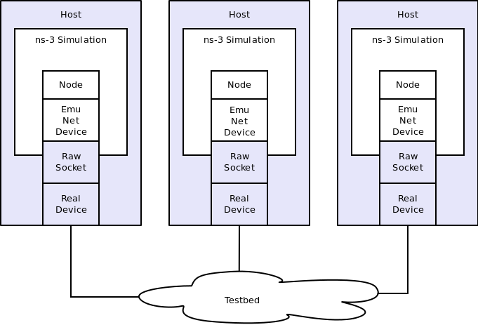
Example Implementation of Testbed Emulation.
You can see that there are separate hosts, each running a subset of a “global” simulation. Instead of an ns-3 channel connecting the hosts, we use real hardware provided by the testbed. This allows ns-3 applications and protocol stacks attached to a simulation node to communicate over real hardware.
We expect the primary use for this configuration will be to generate repeatable experimental results in a real-world network environment that includes all of the ns-3 tracing, logging, visualization and statistics gathering tools.
In what can be viewed as essentially an inverse configuration, we allow “real” machines running native applications and protocol stacks to integrate with an ns-3 simulation. This allows for the simulation of large networks connected to a real machine, and also enables virtualization. A simulation of this kind is shown in the following figure:
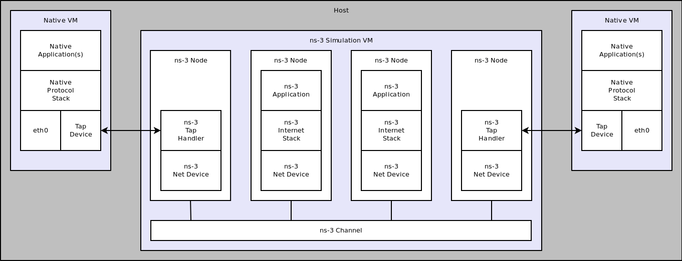
Implementation overview of emulated channel.
Here, you will see that there is a single host with a number of virtual machines running on it. An ns-3 simulation is shown running in the virtual machine shown in the center of the figure. This simulation has a number of nodes with associated ns-3 applications and protocol stacks that are talking to an ns-3 channel through native simulated ns-3 net devices.
There are also two virtual machines shown at the far left and far right of the figure. These VMs are running native (Linux) applications and protocol stacks. The VM is connected into the simulation by a Linux Tap net device. The user-mode handler for the Tap device is instantiated in the simulation and attached to a proxy node that represents the native VM in the simulation. These handlers allow the Tap devices on the native VMs to behave as if they were ns-3 net devices in the simulation VM. This, in turn, allows the native software and protocol suites in the native VMs to believe that they are connected to the simulated ns-3 channel.
We expect the typical use case for this environment will be to analyze the behavior of native applications and protocol suites in the presence of large simulated ns-3 networks.
Emu NetDevice
Behavior
The Emu net device allows a simulation node to send and receive packets over a real network. The emulated net device relies on a specified interface being in promiscuous mode. It opens a raw socket and binds to that interface. We perform MAC spoofing to separate simulation network traffic from other network traffic that may be flowing to and from the host.
One can use the Emu net device in a testbed situation where the host on which the simulation is running has a specific interface of interest which drives the testbed hardware. You would also need to set this specific interface into promiscuous mode and provide an appropriate device name to the ns-3 emulated net device. An example of this environment is the ORBIT testbed as described above.
The Emu net device only works if the underlying interface is up and in promiscuous mode. Packets will be sent out over the device, but we use MAC spoofing. The MAC addresses will be generated (by default) using the Organizationally Unique Identifier (OUI) 00:00:00 as a base. This vendor code is not assigned to any organization and so should not conflict with any real hardware.
It is always up to the user to determine that using these MAC addresses is okay on your network and won’t conflict with anything else (including another simulation using Emu devices) on your network. If you are using the emulated net device in separate simulations you must consider global MAC address assignment issues and ensure that MAC addresses are unique across all simulations. The emulated net device respects the MAC address provided in the SetAddress method so you can do this manually. For larger simulations, you may want to set the OUI in the MAC address allocation function.
IP addresses corresponding to the emulated net devices are the addresses generated in the simulation, which are generated in the usual way via helper functions. Since we are using MAC spoofing, there will not be a conflict between ns-3 network stacks and any native network stacks.
The emulated net device comes with a helper function as all ns-3 devices do. One unique aspect is that there is no channel associated with the underlying medium. We really have no idea what this external medium is, and so have not made an effort to model it abstractly. The primary thing to be aware of is the implication this has for IPv4 global routing. The global router module attempts to walk the channels looking for adjacent networks. Since there is no channel, the global router will be unable to do this and you must then use a dynamic routing protocol such as OLSR to include routing in Emu-based networks.
Usage
Any mixing of ns-3 objects with real objects will typically require that ns-3 compute checksums in its protocols. By default, checksums are not computed by ns-3. To enable checksums (e.g. UDP, TCP, IP), users must set the attribute ChecksumEnabled to true, such as follows::
GlobalValue::Bind ("ChecksumEnabled", BooleanValue (true));
The usage of the Emu net device is straightforward once the network of simulations has been configured. Since most of the work involved in working with this device is in network configuration before even starting a simulation, you may want to take a moment to review a couple of HOWTO pages on the ns-3 wiki that describe how to set up a virtual test network using VMware and how to run a set of example (client server) simulations that use Emu net devices.
- http://www.nsnam.org/wiki/index.php/HOWTO_use_VMware_to_set_up_virtual_networks_(Windows)
- http://www.nsnam.org/wiki/index.php/HOWTO_use_ns-3_scripts_to_drive_real_hardware_(experimental)
Once you are over the configuration hurdle, the script changes required to use an Emu device are trivial. The main structural difference is that you will need to create an ns-3 simulation script for each node. In the case of the HOWTOs above, there is one client script and one server script. The only “challenge” is to get the addresses set correctly.
Just as with all other ns-3 net devices, we provide a helper class for the Emu net device. The following code snippet illustrates how one would declare an EmuHelper and use it to set the “DeviceName” attribute to “eth1” and install Emu devices on a group of nodes. You would do this on both the client and server side in the case of the HOWTO seen above.:
EmuHelper emu;
emu.SetAttribute ("DeviceName", StringValue ("eth1"));
NetDeviceContainer d = emu.Install (n);
The only other change that may be required is to make sure that the address spaces (MAC and IP) on the client and server simulations are compatible. First the MAC address is set to a unique well-known value in both places (illustrated here for one side).:
//
// We've got the devices in place.  Since we're using MAC address
// spoofing under the sheets, we need to make sure that the MAC addresses
// we have assigned to our devices are unique.  Ns-3 will happily
// automatically assign the same MAC address to the devices in both halves
// of our two-script pair, so let's go ahead and just manually change them
// to something we ensure is unique.
//
Ptr<NetDevice> nd = d.Get (0);
Ptr<EmuNetDevice> ed = nd->GetObject<EmuNetDevice> ();
ed->SetAddress ("00:00:00:00:00:02");
And then the IP address of the client or server is set in the usual way using helpers.:
//
// We've got the "hardware" in place.  Now we need to add IP addresses.
// This is the server half of a two-script pair.  We need to make sure
// that the addressing in both of these applications is consistent, so
// we use provide an initial address in both cases.  Here, the client
// will reside on one machine running ns-3 with one node having ns-3
// with IP address "10.1.1.2" and talk to a server script running in
// another ns-3 on another computer that has an ns-3 node with IP
// address "10.1.1.3"
//
Ipv4AddressHelper ipv4;
ipv4.SetBase ("10.1.1.0", "255.255.255.0", "0.0.0.2");
Ipv4InterfaceContainer i = ipv4.Assign (d);
You will use application helpers to generate traffic exactly as you do in any ns-3 simulation script. Note that the server address shown below in a snippet from the client, must correspond to the IP address assigned to the server node similarly to the snippet above.:
uint32_t packetSize = 1024;
uint32_t maxPacketCount = 2000;
Time interPacketInterval = Seconds (0.001);
UdpEchoClientHelper client ("10.1.1.3", 9);
client.SetAttribute ("MaxPackets", UintegerValue (maxPacketCount));
client.SetAttribute ("Interval", TimeValue (interPacketInterval));
client.SetAttribute ("PacketSize", UintegerValue (packetSize));
ApplicationContainer apps = client.Install (n.Get (0));
apps.Start (Seconds (1.0));
apps.Stop (Seconds (2.0));
The Emu net device and helper provide access to ASCII and pcap tracing functionality just as other ns-3 net devices to. You enable tracing similarly to these other net devices::
EmuHelper::EnablePcapAll ("emu-udp-echo-client");
To see an example of a client script using the Emu net device, see examples/emu-udp-echo-client.cc and examples/emu-udp-echo-server.cc in the repository http://code.nsnam.org/craigdo/ns-3-emu/.
Implementation
Perhaps the most unusual part of the Emu and Tap device implementation relates to the requirement for executing some of the code with super-user permissions. Rather than force the user to execute the entire simulation as root, we provide a small “creator” program that runs as root and does any required high-permission sockets work.
We do a similar thing for both the Emu and the Tap devices. The high-level view is that the CreateSocket method creates a local interprocess (Unix) socket, forks, and executes the small creation program. The small program, which runs as suid root, creates a raw socket and sends back the raw socket file descriptor over the Unix socket that is passed to it as a parameter. The raw socket is passed as a control message (sometimes called ancillary data) of type SCM_RIGHTS.
The Emu net device uses the ns-3 threading and multithreaded real-time scheduler extensions. The interesting work in the Emu device is done when the net device is started (EmuNetDevice::StartDevice ()). An attribute (“Start”) provides a simulation time at which to spin up the net device. At this specified time (which defaults to t=0), the socket creation function is called and executes as described above. You may also specify a time at which to stop the device using the “Stop” attribute.
Once the (promiscuous mode) socket is created, we bind it to an interface name also provided as an attribute (“DeviceName”) that is stored internally as m_deviceName::
struct ifreq ifr;
bzero (&ifr, sizeof(ifr));
strncpy ((char *)ifr.ifr_name, m_deviceName.c_str (), IFNAMSIZ);

int32_t rc = ioctl (m_sock, SIOCGIFINDEX, &ifr);

struct sockaddr_ll ll;
bzero (&ll, sizeof(ll));

ll.sll_family = AF_PACKET;
ll.sll_ifindex = m_sll_ifindex;
ll.sll_protocol = htons(ETH_P_ALL);

rc = bind (m_sock, (struct sockaddr *)&ll, sizeof (ll));
After the promiscuous raw socket is set up, a separate thread is spawned to do reads from that socket and the link state is set to Up.:
m_readThread = Create<SystemThread> (
  MakeCallback (&EmuNetDevice::ReadThread, this));
m_readThread->Start ();

NotifyLinkUp ();
The EmuNetDevice::ReadThread function basically just sits in an infinite loop reading from the promiscuous mode raw socket and scheduling packet receptions using the real-time simulator extensions.:
for (;;)
  {
    ...

    len = recvfrom (m_sock, buf, bufferSize, 0, (struct sockaddr *)&addr,
      &addrSize);

    ...

    DynamicCast<RealtimeSimulatorImpl> (Simulator::GetImplementation ())->
      ScheduleRealtimeNow (
        MakeEvent (&EmuNetDevice::ForwardUp, this, buf, len));

    ...
  }
The line starting with our templated DynamicCast function probably deserves a comment. It gains access to the simulator implementation object using the Simulator::GetImplementation method and then casts to the real-time simulator implementation to use the real-time schedule method ScheduleRealtimeNow. This function will cause a handler for the newly received packet to be scheduled for execution at the current real time clock value. This will, in turn cause the simulation clock to be advanced to that real time value when the scheduled event (EmuNetDevice::ForwardUp) is fired.
The ForwardUp function operates as most other similar ns-3 net device methods do. The packet is first filtered based on the destination address. In the case of the Emu device, the MAC destination address will be the address of the Emu device and not the hardware address of the real device. Headers are then stripped off and the trace hooks are hit. Finally, the packet is passed up the ns-3 protocol stack using the receive callback function of the net device.
Sending a packet is equally straightforward as shown below. The first thing we do is to add the ethernet header and trailer to the ns-3 Packet we are sending. The source address corresponds to the address of the Emu device and not the underlying native device MAC address. This is where the MAC address spoofing is done. The trailer is added and we enqueue and dequeue the packet from the net device queue to hit the trace hooks.:
header.SetSource (source);
header.SetDestination (destination);
header.SetLengthType (packet->GetSize ());
packet->AddHeader (header);

EthernetTrailer trailer;
trailer.CalcFcs (packet);
packet->AddTrailer (trailer);

m_queue->Enqueue (packet);
packet = m_queue->Dequeue ();

struct sockaddr_ll ll;
bzero (&ll, sizeof (ll));

ll.sll_family = AF_PACKET;
ll.sll_ifindex = m_sll_ifindex;
ll.sll_protocol = htons(ETH_P_ALL);

rc = sendto (m_sock, packet->PeekData (), packet->GetSize (), 0,
  reinterpret_cast<struct sockaddr *> (&ll), sizeof (ll));
Finally, we simply send the packet to the raw socket which puts it out on the real network.
Tap NetDevice
Placeholder chapter
The Tap NetDevice can be used to allow a host system or virtual machines to interact with a simulation. See examples/tap/tap-wifi-dumbbell.cc for an example.
Internet Models
Sockets APIs
The sockets API is a long-standing API used by user-space applications to access network services in the kernel. A socket is an abstraction, like a Unix file handle, that allows applications to connect to other Internet hosts and exchange reliable byte streams and unreliable datagrams, among other services.
ns-3 provides two types of sockets APIs, and it is important to understand the differences between them. The first is a native ns-3 API, while the second uses the services of the native API to provide a POSIX-like API as part of an overall application process. Both APIs strive to be close to the typical sockets API that application writers on Unix systems are accustomed to, but the POSIX variant is much closer to a real system’s sockets API.
ns-3 sockets API
The native sockets API for ns-3 provides an interface to various types of transport protocols (TCP, UDP) as well as to packet sockets and, in the future, Netlink-like sockets. However, users are cautioned to understand that the semantics are not the exact same as one finds in a real system (for an API which is very much aligned to real systems, see the next section).
ns3::Socket is defined in src/node/socket.h. Readers will note that many public member functions are aligned with real sockets function calls, and all other things being equal, we have tried to align with a Posix sockets API. However, note that:
- ns-3 applications handle a smart pointer to a Socket object, not a file descriptor;
- there is no notion of synchronous API or a blocking API; in fact, the model for interaction between application and socket is one of asynchronous I/O, which is not typically found in real systems (more on this below);
- the C-style socket address structures are not used;
- the API is not a complete sockets API, such as supporting all socket options or all function variants;
- many calls use ns3::Packet class to transfer data between application and socket. This may seem peculiar to pass Packets across a stream socket API, but think of these packets as just fancy byte buffers at this level (more on this also below).
Basic operation and calls
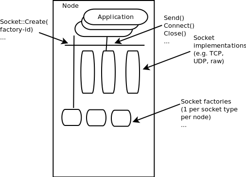
Implementation overview of native sockets API
Creating sockets
An application that wants to use sockets must first create one. On real systems using a C-based API, this is accomplished by calling socket()
int socket(int domain, int type, int protocol);
which creates a socket in the system and returns an integer descriptor.
In ns-3, we have no equivalent of a system call at the lower layers, so we adopt the following model. There are certain factory objects that can create sockets. Each factory is capable of creating one type of socket, and if sockets of a particular type are able to be created on a given node, then a factory that can create such sockets must be aggregated to the Node:
static Ptr<Socket> CreateSocket (Ptr<Node> node, TypeId tid);
Examples of TypeIds to pass to this method are ns3::TcpSocketFactory, ns3::PacketSocketFactory, and ns3::UdpSocketFactory.
This method returns a smart pointer to a Socket object. Here is an example:
Ptr<Node> n0;
// Do some stuff to build up the Node's internet stack
Ptr<Socket> localSocket =
   Socket::CreateSocket (n0, TcpSocketFactory::GetTypeId ());
In some ns-3 code, sockets will not be explicitly created by user’s main programs, if an ns-3 application does it. For instance, for ns3::OnOffApplication, the function ns3::OnOffApplication::StartApplication() performs the socket creation, and the application holds the socket pointer.
Using sockets
Below is a typical sequence of socket calls for a TCP client in a real implementation:
- sock = socket(PF_INET, SOCK_STREAM, IPPROTO_TCP);
- bind(sock, ...);
- connect(sock, ...);
- send(sock, ...);
- recv(sock, ...);
- close(sock);
There are analogs to all of these calls in ns-3, but we will focus on two aspects here. First, most usage of sockets in real systems requires a way to manage I/O between the application and kernel. These models include blocking sockets, signal-based I/O, and non-blocking sockets with polling. In ns-3, we make use of the callback mechanisms to support a fourth mode, which is analogous to POSIX asynchronous I/O.
In this model, on the sending side, if the send() call were to fail because of insufficient buffers, the application suspends the sending of more data until a function registered at the ns3::Socket::SetSendCallback() callback is invoked. An application can also ask the socket how much space is available by calling ns3::Socket::GetTxAvailable(). A typical sequence of events for sending data (ignoring connection setup) might be:
- SetSendCallback (MakeCallback(&HandleSendCallback));
- Send ();
- Send ();
- ...
- Send fails because buffer is full
- wait until HandleSendCallback() is called
- HandleSendCallback() is called by socket, since space now available
- Send (); // Start sending again
Similarly, on the receive side, the socket user does not block on a call to recv(). Instead, the application sets a callback with ns3::Socket::SetRecvCallback() in which the socket will notify the application when (and how much) there is data to be read, and the application then calls ns3::Socket::Recv() to read the data until no more can be read.
Packet vs. buffer variants
There are two basic variants of Send() and Recv() supported:
virtual int Send (Ptr<Packet> p) = 0;
int Send (const uint8_t* buf, uint32_t size);

Ptr<Packet> Recv (void);
int Recv (uint8_t* buf, uint32_t size);
The non-Packet variants are provided for legacy API reasons. When calling the raw buffer variant of ns3::Socket::Send(), the buffer is immediately written into a Packet and the ns3::Socket::Send (Ptr<Packet> p)() is invoked.
Users may find it semantically odd to pass a Packet to a stream socket such as TCP. However, do not let the name bother you; think of ns3::Packet to be a fancy byte buffer. There are a few reasons why the Packet variants are more likely to be preferred in ns-3:
- Users can use the Tags facility of packets to, for example, encode a flow ID or other helper data at the application layer.
- Users can exploit the copy-on-write implementation to avoid memory copies (on the receive side, the conversion back to a uint8_t* buf may sometimes incur an additional copy).
- Use of Packet is more aligned with the rest of the ns-3 API
Sending dummy data
Sometimes, users want the simulator to just pretend that there is an actual data payload in the packet (e.g. to calculate transmission delay) but do not want to actually produce or consume the data. This is straightforward to support in ns-3; have applications call Create<Packet> (size); instead of Create<Packet> (buffer, size);. Similarly, passing in a zero to the pointer argument in the raw buffer variants has the same effect. Note that, if some subsequent code tries to read the Packet data buffer, the fake buffer will be converted to a real (zeroed) buffer on the spot, and the efficiency will be lost there.
Socket options
to be completed
Socket errno
to be completed
Example programs
to be completed
POSIX-like sockets API
Internet Stack
Internet stack aggregation
A bare class Node is not very useful as-is; other objects must be aggregated to it to provide useful node functionality.
The ns-3 source code directory src/internet-stack provides implementation of TCP/IPv4- and IPv6-related components. These include IPv4, ARP, UDP, TCP, IPv6, Neighbor Discovery, and other related protocols.
Internet Nodes are not subclasses of class Node; they are simply Nodes that have had a bunch of IPv4-related objects aggregated to them. They can be put together by hand, or via a helper function InternetStackHelper::Install () which does the following to all nodes passed in as arguments::
void
InternetStackHelper::Install (Ptr<Node> node) const
{
  if (node->GetObject<Ipv4> () != 0)
    {
      NS_FATAL_ERROR ("InternetStackHelper::Install(): Aggregating "
                      "an InternetStack to a node with an existing Ipv4 object");
      return;
    }

  CreateAndAggregateObjectFromTypeId (node, "ns3::ArpL3Protocol");
  CreateAndAggregateObjectFromTypeId (node, "ns3::Ipv4L3Protocol");
  CreateAndAggregateObjectFromTypeId (node, "ns3::Icmpv4L4Protocol");
  CreateAndAggregateObjectFromTypeId (node, "ns3::UdpL4Protocol");
  node->AggregateObject (m_tcpFactory.Create<Object> ());
  Ptr<PacketSocketFactory> factory = CreateObject<PacketSocketFactory> ();
  node->AggregateObject (factory);
  // Set routing
  Ptr<Ipv4> ipv4 = node->GetObject<Ipv4> ();
  Ptr<Ipv4RoutingProtocol> ipv4Routing = m_routing->Create (node);
  ipv4->SetRoutingProtocol (ipv4Routing);
}
Where multiple implementations exist in ns-3 (TCP, IP routing), these objects are added by a factory object (TCP) or by a routing helper (m_routing).
Note that the routing protocol is configured and set outside this function. By default, the following protocols are added to Ipv4::
InternetStackHelper::InternetStackHelper ()
{
  SetTcp ("ns3::TcpL4Protocol");
  static Ipv4StaticRoutingHelper staticRouting;
  static Ipv4GlobalRoutingHelper globalRouting;
  static Ipv4ListRoutingHelper listRouting;
  listRouting.Add (staticRouting, 0);
  listRouting.Add (globalRouting, -10);
  SetRoutingHelper (listRouting);
}
By default, IPv4 and IPv6 are enabled.
Internet Node structure
An IPv4-capable Node (an ns-3 Node augmented by aggregation to have one or more IP stacks) has the following internal structure.
Layer-3 protocols
At the lowest layer, sitting above the NetDevices, are the “layer 3” protocols, including IPv4, IPv6 (in the future), and ARP. The class Ipv4L3Protocol is an implementation class whose public interface is typically class Ipv4 (found in src/node directory), but the Ipv4L3Protocol public API is also used internally in the src/internet-stack directory at present.
In class Ipv4L3Protocol, one method described below is Receive ()::
 /**
   * Lower layer calls this method after calling L3Demux::Lookup
   * The ARP subclass needs to know from which NetDevice this
   * packet is coming to:
   *    - implement a per-NetDevice ARP cache
   *    - send back arp replies on the right device
   */
  void Receive( Ptr<NetDevice> device, Ptr<const Packet> p, uint16_t protocol,
const Address &from, const Address &to, NetDevice::PacketType packetType);
First, note that the Receive () function has a matching signature to the ReceiveCallback in the class Node. This function pointer is inserted into the Node’s protocol handler when AddInterface () is called. The actual registration is done with a statement such as follows::
RegisterProtocolHandler ( MakeCallback (&Ipv4Protocol::Receive, ipv4),
   Ipv4L3Protocol::PROT_NUMBER, 0);
The Ipv4L3Protocol object is aggregated to the Node; there is only one such Ipv4L3Protocol object. Higher-layer protocols that have a packet to send down to the Ipv4L3Protocol object can call GetObject<Ipv4L3Protocol> () to obtain a pointer, as follows::
Ptr<Ipv4L3Protocol> ipv4 = m_node->GetObject<Ipv4L3Protocol> ();
if (ipv4 != 0)
  {
    ipv4->Send (packet, saddr, daddr, PROT_NUMBER);
  }
This class nicely demonstrates two techniques we exploit in ns-3 to bind objects together: callbacks, and object aggregation.
Once IPv4 routing has determined that a packet is for the local node, it forwards it up the stack. This is done with the following function::
void
Ipv4L3Protocol::LocalDeliver (Ptr<const Packet> packet, Ipv4Header const&ip, uint32_t iif)
The first step is to find the right Ipv4L4Protocol object, based on IP protocol number. For instance, TCP is registered in the demux as protocol number 6. Finally, the Receive() function on the Ipv4L4Protocol (such as TcpL4Protocol::Receive is called.
We have not yet introduced the class Ipv4Interface. Basically, each NetDevice is paired with an IPv4 representation of such device. In Linux, this class Ipv4Interface roughly corresponds to the struct in_device; the main purpose is to provide address-family specific information (addresses) about an interface.
The IPv6 implementation follows a similar architecture.
Layer-4 protocols and sockets
We next describe how the transport protocols, sockets, and applications tie together. In summary, each transport protocol implementation is a socket factory. An application that needs a new socket
For instance, to create a UDP socket, an application would use a code snippet such as the following::
Ptr<Udp> udpSocketFactory = GetNode ()->GetObject<Udp> ();
Ptr<Socket> m_socket = socketFactory->CreateSocket ();
m_socket->Bind (m_local_address);
...
The above will query the node to get a pointer to its UDP socket factory, will create one such socket, and will use the socket with an API similar to the C-based sockets API, such as Connect () and Send (). See the chapter on ns-3 sockets for more information.
We have described so far a socket factory (e.g. class Udp) and a socket, which may be specialized (e.g., class UdpSocket). There are a few more key objects that relate to the specialized task of demultiplexing a packet to one or more receiving sockets. The key object in this task is class Ipv4EndPointDemux. This demultiplexer stores objects of class Ipv4EndPoint. This class holds the addressing/port tuple (local port, local address, destination port, destination address) associated with the socket, and a receive callback. This receive callback has a receive function registered by the socket. The Lookup () function to Ipv4EndPointDemux returns a list of Ipv4EndPoint objects (there may be a list since more than one socket may match the packet). The layer-4 protocol copies the packet to each Ipv4EndPoint and calls its ForwardUp () method, which then calls the Receive () function registered by the socket.
An issue that arises when working with the sockets API on real systems is the need to manage the reading from a socket, using some type of I/O (e.g., blocking, non-blocking, asynchronous, ...). ns-3 implements an asynchronous model for socket I/O; the application sets a callback to be notified of received data ready to be read, and the callback is invoked by the transport protocol when data is available. This callback is specified as follows::
void Socket::SetRecvCallback (Callback<void, Ptr<Socket>,
  Ptr<Packet>, const Address&> receivedData);
The data being received is conveyed in the Packet data buffer. An example usage is in class PacketSink::
m_socket->SetRecvCallback (MakeCallback(&PacketSink::HandleRead, this));
To summarize, internally, the UDP implementation is organized as follows:
- a UdpImpl class that implements the UDP socket factory functionality
- a UdpL4Protocol class that implements the protocol logic that is socket-independent
- a UdpSocketImpl class that implements socket-specific aspects of UDP
- a class called Ipv4EndPoint that stores the addressing tuple (local port, local address, destination port, destination address) associated with the socket, and a receive callback for the socket.
Ipv4-capable node interfaces
Many of the implementation details, or internal objects themselves, of Ipv4-capable Node objects are not exposed at the simulator public API. This allows for different implementations; for instance, replacing the native ns-3 models with ported TCP/IP stack code.
The C++ public APIs of all of these objects is found in the src/node directory, including principally:
- socket.h
- tcp.h
- udp.h
- ipv4.h
These are typically base class objects that implement the default values used in the implementation, implement access methods to get/set state variables, host attributes, and implement publicly-available methods exposed to clients such as CreateSocket.
Example path of a packet
These two figures show an example stack trace of how packets flow through the Internet Node objects.
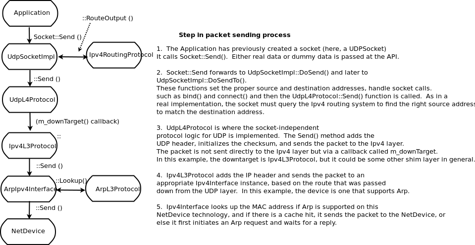
Send path of a packet.
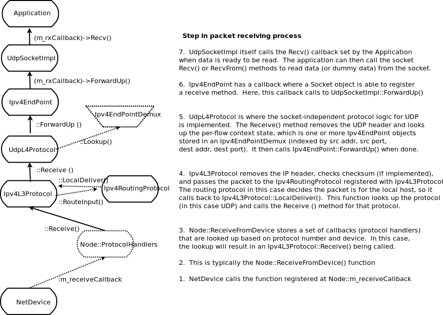
Receive path of a packet.
IPv4
Placeholder chapter
IPv6
Placeholder chapter
IPv6 models are being added to ns-3. A paper on the IPv6 models was published in WNS2 2008: http://lsiit.u-strasbg.fr/Publications/2008/VMM08/.
Routing overview
ns-3 is intended to support traditional routing approaches and protocols, support ports of open source routing implementations, and facilitate research into unorthodox routing techniques. The overall routing architecture is described below in Routing architecture. Users who wish to just read about how to configure global routing for wired topologies can read Global centralized routing. Unicast routing protocols are described in Unicast routing. Multicast routing is documented in Multicast routing.
Routing architecture
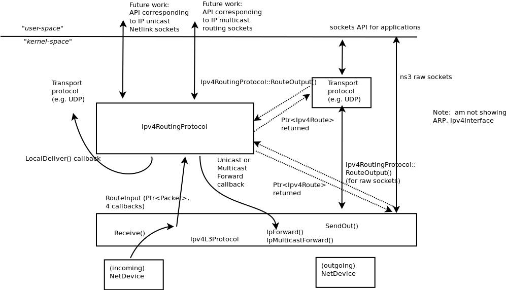
Overview of routing
Overview of routing shows the overall routing architecture for Ipv4. The key objects are Ipv4L3Protocol, Ipv4RoutingProtocol(s) (a class to which all routing/forwarding has been delegated from Ipv4L3Protocol), and Ipv4Route(s).
Ipv4L3Protocol must have at least one Ipv4RoutingProtocol added to it at simulation setup time. This is done explicitly by calling Ipv4::SetRoutingProtocol ().
The abstract base class Ipv4RoutingProtocol () declares a minimal interface, consisting of two methods: RouteOutput () and RouteInput (). For packets traveling outbound from a host, the transport protocol will query Ipv4 for the Ipv4RoutingProtocol object interface, and will request a route via Ipv4RoutingProtocol::RouteOutput (). A Ptr to Ipv4Route object is returned. This is analagous to a dst_cache entry in Linux. The Ipv4Route is carried down to the Ipv4L3Protocol to avoid a second lookup there. However, some cases (e.g. Ipv4 raw sockets) will require a call to RouteOutput() directly from Ipv4L3Protocol.
For packets received inbound for forwarding or delivery, the following steps occur. Ipv4L3Protocol::Receive() calls Ipv4RoutingProtocol::RouteInput(). This passes the packet ownership to the Ipv4RoutingProtocol object. There are four callbacks associated with this call:
- LocalDeliver
- UnicastForward
- MulticastForward
- Error
The Ipv4RoutingProtocol must eventually call one of these callbacks for each packet that it takes responsibility for. This is basically how the input routing process works in Linux.
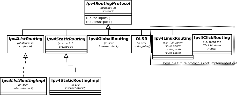
Ipv4Routing specialization.
This overall architecture is designed to support different routing approaches, including (in the future) a Linux-like policy-based routing implementation, proactive and on-demand routing protocols, and simple routing protocols for when the simulation user does not really care about routing.
Ipv4Routing specialization. illustrates how multiple routing protocols derive from this base class. A class Ipv4ListRouting (implementation class Ipv4ListRoutingImpl) provides the existing list routing approach in ns-3. Its API is the same as base class Ipv4Routing except for the ability to add multiple prioritized routing protocols (Ipv4ListRouting::AddRoutingProtocol(), Ipv4ListRouting::GetRoutingProtocol()).
The details of these routing protocols are described below in Unicast routing. For now, we will first start with a basic unicast routing capability that is intended to globally build routing tables at simulation time t=0 for simulation users who do not care about dynamic routing.
Global centralized routing
Global centralized routing is sometimes called “God” routing; it is a special implementation that walks the simulation topology and runs a shortest path algorithm, and populates each node’s routing tables. No actual protocol overhead (on the simulated links) is incurred with this approach. It does have a few constraints:
- Wired only: It is not intended for use in wireless networks.
- Unicast only: It does not do multicast.
- Scalability: Some users of this on large topologies (e.g. 1000 nodes) have noticed that the current implementation is not very scalable. The global centralized routing will be modified in the future to reduce computations and runtime performance.
Presently, global centralized IPv4 unicast routing over both point-to-point and shared (CSMA) links is supported.
By default, when using the ns-3 helper API and the default InternetStackHelper, global routing capability will be added to the node, and global routing will be inserted as a routing protocol with lower priority than the static routes (i.e., users can insert routes via Ipv4StaticRouting API and they will take precedence over routes found by global routing).
Global Unicast Routing API
The public API is very minimal. User scripts include the following::
#include "ns3/helper-module.h"
If the default InternetStackHelper is used, then an instance of global routing will be aggregated to each node. After IP addresses are configured, the following function call will cause all of the nodes that have an Ipv4 interface to receive forwarding tables entered automatically by the GlobalRouteManager::
Ipv4GlobalRoutingHelper::PopulateRoutingTables ();
Note: A reminder that the wifi NetDevice will work but does not take any wireless effects into account. For wireless, we recommend OLSR dynamic routing described below.
It is possible to call this function again in the midst of a simulation using the following additional public function::
Ipv4GlobalRoutingHelper::RecomputeRoutingTables ();
which flushes the old tables, queries the nodes for new interface information, and rebuilds the routes.
For instance, this scheduling call will cause the tables to be rebuilt at time 5 seconds::
Simulator::Schedule (Seconds (5),
  &Ipv4GlobalRoutingHelper::RecomputeRoutingTables);
There are two attributes that govern the behavior. The first is Ipv4GlobalRouting::RandomEcmpRouting. If set to true, packets are randomly routed across equal-cost multipath routes. If set to false (default), only one route is consistently used. The second is Ipv4GlobalRouting::RespondToInterfaceEvents. If set to true, dynamically recompute the global routes upon Interface notification events (up/down, or add/remove address). If set to false (default), routing may break unless the user manually calls RecomputeRoutingTables() after such events. The default is set to false to preserve legacy ns-3 program behavior.
Global Routing Implementation
This section is for those readers who care about how this is implemented. A singleton object (GlobalRouteManager) is responsible for populating the static routes on each node, using the public Ipv4 API of that node. It queries each node in the topology for a “globalRouter” interface. If found, it uses the API of that interface to obtain a “link state advertisement (LSA)” for the router. Link State Advertisements are used in OSPF routing, and we follow their formatting.
The GlobalRouteManager populates a link state database with LSAs gathered from the entire topology. Then, for each router in the topology, the GlobalRouteManager executes the OSPF shortest path first (SPF) computation on the database, and populates the routing tables on each node.
The quagga (http://www.quagga.net) OSPF implementation was used as the basis for the routing computation logic. One benefit of following an existing OSPF SPF implementation is that OSPF already has defined link state advertisements for all common types of network links:
- point-to-point (serial links)
- point-to-multipoint (Frame Relay, ad hoc wireless)
- non-broadcast multiple access (ATM)
- broadcast (Ethernet)
Therefore, we think that enabling these other link types will be more straightforward now that the underlying OSPF SPF framework is in place.
Presently, we can handle IPv4 point-to-point, numbered links, as well as shared broadcast (CSMA) links, and we do not do equal-cost multipath.
The GlobalRouteManager first walks the list of nodes and aggregates a GlobalRouter interface to each one as follows::
typedef std::vector < Ptr<Node> >::iterator Iterator;
for (Iterator i = NodeList::Begin (); i != NodeList::End (); i++)
  {
    Ptr<Node> node = *i;
    Ptr<GlobalRouter> globalRouter = CreateObject<GlobalRouter> (node);
    node->AggregateObject (globalRouter);
  }
This interface is later queried and used to generate a Link State Advertisement for each router, and this link state database is fed into the OSPF shortest path computation logic. The Ipv4 API is finally used to populate the routes themselves.
Unicast routing
There are presently seven unicast routing protocols defined for IPv4 and two for IPv6:
- class Ipv4StaticRouting (covering both unicast and multicast)
- IPv4 Optimized Link State Routing (OLSR) (a MANET protocol defined in RFC 3626)
- IPv4 Ad Hoc On Demand Distance Vector (AODV) (a MANET protocol defined in RFC 3561)
- IPv4 Destination Sequenced Distance Vector (DSDV) (a MANET protocol)
- class Ipv4ListRouting (used to store a prioritized list of routing protocols)
- class Ipv4GlobalRouting (used to store routes computed by the global route manager, if that is used)
- class Ipv4NixVectorRouting (a more efficient version of global routing that stores source routes in a packet header field)
- class Ipv6ListRouting (used to store a prioritized list of routing protocols)
- class Ipv6StaticRouting
In the future, this architecture should also allow someone to implement a Linux-like implementation with routing cache, or a Click modular router, but those are out of scope for now.
Ipv4ListRouting
This section describes the current default ns-3 Ipv4RoutingProtocol. Typically, multiple routing protocols are supported in user space and coordinate to write a single forwarding table in the kernel. Presently in ns-3, the implementation instead allows for multiple routing protocols to build/keep their own routing state, and the IPv4 implementation will query each one of these routing protocols (in some order determined by the simulation author) until a route is found.
We chose this approach because it may better facilitate the integration of disparate routing approaches that may be difficult to coordinate the writing to a single table, approaches where more information than destination IP address (e.g., source routing) is used to determine the next hop, and on-demand routing approaches where packets must be cached.
Ipv4ListRouting::AddRoutingProtocol
Class Ipv4ListRouting provides a pure virtual function declaration for the method that allows one to add a routing protocol::
void AddRoutingProtocol (Ptr<Ipv4RoutingProtocol> routingProtocol,
                         int16_t priority);
This method is implemented by class Ipv4ListRoutingImpl in the internet-stack module.
The priority variable above governs the priority in which the routing protocols are inserted. Notice that it is a signed int. By default in ns-3, the helper classes will instantiate a Ipv4ListRoutingImpl object, and add to it an Ipv4StaticRoutingImpl object at priority zero. Internally, a list of Ipv4RoutingProtocols is stored, and and the routing protocols are each consulted in decreasing order of priority to see whether a match is found. Therefore, if you want your Ipv4RoutingProtocol to have priority lower than the static routing, insert it with priority less than 0; e.g.::
Ptr<MyRoutingProtocol> myRoutingProto = CreateObject<MyRoutingProtocol> ();
listRoutingPtr->AddRoutingProtocol (myRoutingProto, -10);
Upon calls to RouteOutput() or RouteInput(), the list routing object will search the list of routing protocols, in priority order, until a route is found. Such routing protocol will invoke the appropriate callback and no further routing protocols will be searched.
Optimized Link State Routing (OLSR)
This IPv4 routing protocol was originally ported from the OLSR-UM implementation for ns-2. The implementation is found in the src/routing/olsr directory, and an example script is in examples/simple-point-to-point-olsr.cc.
Typically, OLSR is enabled in a main program by use of an OlsrHelper class that installs OLSR into an Ipv4ListRoutingProtocol object. The following sample commands will enable OLSR in a simulation using this helper class along with some other routing helper objects. The setting of priority value 10, ahead of the staticRouting priority of 0, means that OLSR will be consulted for a route before the node’s static routing table.:
NodeContainer c:
...
// Enable OLSR
NS_LOG_INFO ("Enabling OLSR Routing.");
OlsrHelper olsr;

Ipv4StaticRoutingHelper staticRouting;

Ipv4ListRoutingHelper list;
list.Add (staticRouting, 0);
list.Add (olsr, 10);

InternetStackHelper internet;
internet.SetRoutingHelper (list);
internet.Install (c);
Once installed,the OLSR “main interface” can be set with the SetMainInterface() command. If the user does not specify a main address, the protocol will select the first primary IP address that it finds, starting first the loopback interface and then the next non-loopback interface found, in order of Ipv4 interface index. The loopback address of 127.0.0.1 is not selected. In addition, a number of protocol constants are defined in olsr-routing-protocol.cc.
Olsr is started at time zero of the simulation, based on a call to Object::Start() that eventually calls OlsrRoutingProtocol::DoStart(). Note: a patch to allow the user to start and stop the protocol at other times would be welcome.
Presently, OLSR is limited to use with an Ipv4ListRouting object, and does not respond to dynamic changes to a device’s IP address or link up/down notifications; i.e. the topology changes are due to loss/gain of connectivity over a wireless channel.
Multicast routing
The following function is used to add a static multicast route to a node::
void
Ipv4StaticRouting::AddMulticastRoute (Ipv4Address origin,
                          Ipv4Address group,
                          uint32_t inputInterface,
                          std::vector<uint32_t> outputInterfaces);
A multicast route must specify an origin IP address, a multicast group and an input network interface index as conditions and provide a vector of output network interface indices over which packets matching the conditions are sent.
Typically there are two main types of multicast routes: routes of the first kind are used during forwarding. All of the conditions must be explicitly provided. The second kind of routes are used to get packets off of a local node. The difference is in the input interface. Routes for forwarding will always have an explicit input interface specified. Routes off of a node will always set the input interface to a wildcard specified by the index Ipv4RoutingProtocol::IF_INDEX_ANY.
For routes off of a local node wildcards may be used in the origin and multicast group addresses. The wildcard used for Ipv4Adresses is that address returned by Ipv4Address::GetAny () – typically “0.0.0.0”. Usage of a wildcard allows one to specify default behavior to varying degrees.
For example, making the origin address a wildcard, but leaving the multicast group specific allows one (in the case of a node with multiple interfaces) to create different routes using different output interfaces for each multicast group.
If the origin and multicast addresses are made wildcards, you have created essentially a default multicast address that can forward to multiple interfaces. Compare this to the actual default multicast address that is limited to specifying a single output interface for compatibility with existing functionality in other systems.
Another command sets the default multicast route::
void
Ipv4StaticRouting::SetDefaultMulticastRoute (uint32_t outputInterface);
This is the multicast equivalent of the unicast version SetDefaultRoute. We tell the routing system what to do in the case where a specific route to a destination multicast group is not found. The system forwards packets out the specified interface in the hope that “something out there” knows better how to route the packet. This method is only used in initially sending packets off of a host. The default multicast route is not consulted during forwarding – exact routes must be specified using AddMulticastRoute for that case.
Since we’re basically sending packets to some entity we think may know better what to do, we don’t pay attention to “subtleties” like origin address, nor do we worry about forwarding out multiple interfaces. If the default multicast route is set, it is returned as the selected route from LookupStatic irrespective of origin or multicast group if another specific route is not found.
Finally, a number of additional functions are provided to fetch and remove multicast routes::
uint32_t GetNMulticastRoutes (void) const;

Ipv4MulticastRoute *GetMulticastRoute (uint32_t i) const;

Ipv4MulticastRoute *GetDefaultMulticastRoute (void) const;

bool RemoveMulticastRoute (Ipv4Address origin,
                           Ipv4Address group,
                           uint32_t inputInterface);

void RemoveMulticastRoute (uint32_t index);
TCP models in ns-3
This chapter describes the TCP models available in ns-3.
Generic support for TCP
ns-3 was written to support multiple TCP implementations. The implementations inherit from a few common header classes in the src/node directory, so that user code can swap out implementations with minimal changes to the scripts.
There are two important abstract base classes:
- class TcpSocket: This is defined in src/node/tcp-socket.{cc,h}. This class exists for hosting TcpSocket attributes that can be reused across different implementations. For instance, the attribute InitialCwnd can be used for any of the implementations that derive from class TcpSocket.
- class TcpSocketFactory: This is used by the layer-4 protocol instance to create TCP sockets of the right type.
There are presently two implementations of TCP available for ns-3.
- a natively implemented TCP for ns-3
- support for the Network Simulation Cradle (NSC)
It should also be mentioned that various ways of combining virtual machines with ns-3 makes available also some additional TCP implementations, but those are out of scope for this chapter.
ns-3 TCP
Until ns-3.10 release, ns-3 contained a port of the TCP model from GTNetS. This implementation was substantially rewritten by Adriam Tam for ns-3.10. The model is a full TCP, in that it is bidirectional and attempts to model the connection setup and close logic.
The implementation of TCP is contained in the following files::
src/internet-stack/tcp-header.{cc,h}
src/internet-stack/tcp-l4-protocol.{cc,h}
src/internet-stack/tcp-socket-factory-impl.{cc,h}
src/internet-stack/tcp-socket-base.{cc,h}
src/internet-stack/tcp-tx-buffer.{cc,h}
src/internet-stack/tcp-rx-buffer.{cc,h}
src/internet-stack/tcp-rfc793.{cc,h}
src/internet-stack/tcp-tahoe.{cc,h}
src/internet-stack/tcp-reno.{cc,h}
src/internet-stack/tcp-newreno.{cc,h}
src/internet-stack/rtt-estimator.{cc,h}
src/common/sequence-number.{cc,h}
Different variants of TCP congestion control are supported by subclassing the common base class TcpSocketBase. Several variants are supported, including RFC 793 (no congestion control), Tahoe, Reno, and NewReno. NewReno is used by default.
Usage
In many cases, usage of TCP is set at the application layer by telling the ns-3 application which kind of socket factory to use.
Using the helper functions defined in src/helper, here is how one would create a TCP receiver::
// Create a packet sink on the star "hub" to receive these packets
uint16_t port = 50000;
Address sinkLocalAddress(InetSocketAddress (Ipv4Address::GetAny (), port));
PacketSinkHelper sinkHelper ("ns3::TcpSocketFactory", sinkLocalAddress);
ApplicationContainer sinkApp = sinkHelper.Install (serverNode);
sinkApp.Start (Seconds (1.0));
sinkApp.Stop (Seconds (10.0));
Similarly, the below snippet configures OnOffApplication traffic source to use TCP::
// Create the OnOff applications to send TCP to the server
OnOffHelper clientHelper ("ns3::TcpSocketFactory", Address ());
The careful reader will note above that we have specified the TypeId of an abstract base class TcpSocketFactory. How does the script tell ns-3 that it wants the native ns-3 TCP vs. some other one? Well, when internet stacks are added to the node, the default TCP implementation that is aggregated to the node is the ns-3 TCP. This can be overridden as we show below when using Network Simulation Cradle. So, by default, when using the ns-3 helper API, the TCP that is aggregated to nodes with an Internet stack is the native ns-3 TCP.
To configure behavior of TCP, a number of parameters are exported through the Attributes. These are documented in the Doxygen <http://www.nsnam.org/doxygen/classns3_1_1_tcp_socket.html> for class TcpSocket. For example, the maximum segment size is a settable attribute.
For users who wish to have a pointer to the actual socket (so that socket operations like Bind(), setting socket options, etc. can be done on a per-socket basis), Tcp sockets can be created by using the Socket::CreateSocket() method and passing in the TypeId corresponding to the type of socket desired; e.g.::
// Create the socket if not already created
TypeId tid = TypeId::LookupByName ("ns3::TcpTahoe");
Ptr<Socket> localSocket = Socket::CreateSocket (node, tid);
The parameter tid controls the TypeId of the actual TCP Socket implementation that is instantiated. This way, the application can be written generically and different socket implementations can be swapped out by specifying the TypeId.
Once a TCP socket is created, one will want to follow conventional socket logic and either connect() and send() (for a TCP client) or bind(), listen(), and accept() (for a TCP server). Sockets API for a review of how sockets are used in ns-3.
Validation
Several TCP validation test results can be found in the wiki page describing this implementation.
Current limitations
- Only IPv4 is supported
- Neither the Nagle algorithm nor SACK are supported
Network Simulation Cradle
The Network Simulation Cradle (NSC) is a framework for wrapping real-world network code into simulators, allowing simulation of real-world behavior at little extra cost. This work has been validated by comparing situations using a test network with the same situations in the simulator. To date, it has been shown that the NSC is able to produce extremely accurate results. NSC supports four real world stacks: FreeBSD, OpenBSD, lwIP and Linux. Emphasis has been placed on not changing any of the network stacks by hand. Not a single line of code has been changed in the network protocol implementations of any of the above four stacks. However, a custom C parser was built to programmatically change source code.
NSC has previously been ported to ns-2 and OMNeT++, and recently was added to ns-3. This section describes the ns-3 port of NSC and how to use it.
Prerequisites
Presently, NSC has been tested and shown to work on these platforms: Linux i386 and Linux x86-64. NSC does not support powerpc.
Building NSC requires the packages flex and bison.
Configuring and Downloading
Using the build.py script in ns-3-allinone directory, NSC will be enabled by default unless the platform does not support it. To disable it when building ns-3, type::
./waf configure --disable-nsc
Building and validating
Building ns-3 with nsc support is the same as building it without; no additional arguments are needed for waf. Building nsc may take some time compared to ns-3; it is interleaved in the ns-3 building process.
Try running the following ns-3 test suite::
./test.py -s ns3-tcp-interoperability
If NSC has been successfully built, the following test should show up in the results::
PASS TestSuite ns3-tcp-interoperability
This confirms that NSC is ready to use.
Usage
There are a few example files. Try:
./waf --run tcp-nsc-zoo
./waf --run tcp-nsc-lfn
These examples will deposit some .pcap files in your directory, which can be examined by tcpdump or wireshark.
Let’s look at the examples/tcp-nsc-zoo.cc file for some typical usage. How does it differ from using native ns-3 TCP? There is one main configuration line, when using NSC and the ns-3 helper API, that needs to be set::
InternetStackHelper internetStack;

internetStack.SetNscStack ("liblinux2.6.26.so");
// this switches nodes 0 and 1 to NSCs Linux 2.6.26 stack.
internetStack.Install (n.Get(0));
internetStack.Install (n.Get(1));
The key line is the SetNscStack. This tells the InternetStack helper to aggregate instances of NSC TCP instead of native ns-3 TCP to the remaining nodes. It is important that this function be called before calling the Install() function, as shown above.
Which stacks are available to use? Presently, the focus has been on Linux 2.6.18 and Linux 2.6.26 stacks for ns-3. To see which stacks were built, one can execute the following find command at the ns-3 top level directory::
~/ns-3.10> find nsc -name "*.so" -type f
nsc/linux-2.6.18/liblinux2.6.18.so
nsc/linux-2.6.26/liblinux2.6.26.so
This tells us that we may either pass the library name liblinux2.6.18.so or liblinux2.6.26.so to the above configuration step.
Stack configuration
NSC TCP shares the same configuration attributes that are common across TCP sockets, as described above and documented in Doxygen
Additionally, NSC TCP exports a lot of configuration variables into the ns-3 Attributes system, via a sysctl-like interface. In the examples/tcp-nsc-zoo example, you can see the following configuration::
// this disables TCP SACK, wscale and timestamps on node 1 (the attributes
  represent sysctl-values).
Config::Set ("/NodeList/1/$ns3::Ns3NscStack<linux2.6.26>/net.ipv4.tcp_sack",
  StringValue ("0"));
Config::Set ("/NodeList/1/$ns3::Ns3NscStack<linux2.6.26>/net.ipv4.tcp_timestamps",
StringValue ("0"));
Config::Set ("/NodeList/1/$ns3::Ns3NscStack<linux2.6.26>/net.ipv4.tcp_window_scaling",
StringValue ("0"));
These additional configuration variables are not available to native ns-3 TCP.
NSC API
This subsection describes the API that NSC presents to ns-3 or any other simulator. NSC provides its API in the form of a number of classes that are defined in sim/sim_interface.h in the nsc directory.
- INetStack INetStack contains the ‘low level’ operations for the operating system network stack, e.g. in and output functions from and to the network stack (think of this as the ‘network driver interface’. There are also functions to create new TCP or UDP sockets.
- ISendCallback This is called by NSC when a packet should be sent out to the network. This simulator should use this callback to re-inject the packet into the simulator so the actual data can be delivered/routed to its destination, where it will eventually be handed into Receive() (and eventually back to the receivers NSC instance via INetStack->if_receive() ).
- INetStreamSocket This is the structure defining a particular connection endpoint (file descriptor). It contains methods to operate on this endpoint, e.g. connect, disconnect, accept, listen, send_data/read_data, ...
- IInterruptCallback This contains the wakeup callback, which is called by NSC whenever something of interest happens. Think of wakeup() as a replacement of the operating systems wakeup function: Whenever the operating system would wake up a process that has been waiting for an operation to complete (for example the TCP handshake during connect()), NSC invokes the wakeup() callback to allow the simulator to check for state changes in its connection endpoints.
ns-3 implementation
The ns-3 implementation makes use of the above NSC API, and is implemented as follows.
The three main parts are:
- ns3::NscTcpL4Protocol: a subclass of Ipv4L4Protocol (and two nsc classes: ISendCallback and IInterruptCallback)
- ns3::NscTcpSocketImpl: a subclass of TcpSocket
- ns3::NscTcpSocketFactoryImpl: a factory to create new NSC sockets
src/internet-stack/nsc-tcp-l4-protocol is the main class. Upon Initialization, it loads an nsc network stack to use (via dlopen()). Each instance of this class may use a different stack. The stack (=shared library) to use is set using the SetNscLibrary() method (at this time its called indirectly via the internet stack helper). The nsc stack is then set up accordingly (timers etc). The NscTcpL4Protocol::Receive() function hands the packet it receives (must be a complete tcp/ip packet) to the nsc stack for further processing. To be able to send packets, this class implements the nsc send_callback method. This method is called by nsc whenever the nsc stack wishes to send a packet out to the network. Its arguments are a raw buffer, containing a complete TCP/IP packet, and a length value. This method therefore has to convert the raw data to a Ptr<Packet> usable by ns-3. In order to avoid various ipv4 header issues, the nsc ip header is not included. Instead, the tcp header and the actual payload are put into the Ptr<Packet>, after this the Packet is passed down to layer 3 for sending the packet out (no further special treatment is needed in the send code path).
This class calls ns3::NscTcpSocketImpl both from the nsc wakeup() callback and from the Receive path (to ensure that possibly queued data is scheduled for sending).
src/internet-stack/nsc-tcp-socket-impl implements the nsc socket interface. Each instance has its own nscTcpSocket. Data that is Send() will be handed to the nsc stack via m_nscTcpSocket->send_data(). (and not to nsc-tcp-l4, this is the major difference compared to ns-3 TCP). The class also queues up data that is Send() before the underlying descriptor has entered an ESTABLISHED state. This class is called from the nsc-tcp-l4 class, when the nsc-tcp-l4 wakeup() callback is invoked by nsc. nsc-tcp-socket-impl then checks the current connection state (SYN_SENT, ESTABLISHED, LISTEN...) and schedules appropriate callbacks as needed, e.g. a LISTEN socket will schedule Accept to see if a new connection must be accepted, an ESTABLISHED socket schedules any pending data for writing, schedule a read callback, etc.
Note that ns3::NscTcpSocketImpl does not interact with nsc-tcp directly: instead, data is redirected to nsc. nsc-tcp calls the nsc-tcp-sockets of a node when its wakeup callback is invoked by nsc.
Limitations
- NSC only works on single-interface nodes; attempting to run it on a multi-interface node will cause a program error.
- Cygwin and OS X PPC are not supported
- The non-Linux stacks of NSC are not supported in ns-3
- Not all socket API callbacks are supported
For more information, see this wiki page.
Applications
Placeholder chapter
Support
Flow Monitor
Placeholder chapter
This feature was added as contributed code (src/contrib) in ns-3.6 and to the main distribution for ns-3.7. A paper on this feature is published in the proceedings of NSTools: http://www.nstools.org/techprog.shtml.
Animation
Animation is an important tool for network simulation. While ns-3 does not contain a default graphical animation tool, it does provide an animation interface for use with stand-alone animators. One such animator called NetAnim, presently supporting packet flow animation for point-to-point links, has been developed. Other animators and visualization tools are in development; they may make use of the existing animation interface or may develop new ones,
Animation interface
The animation interface uses underlying ns-3 trace sources to construct a timestamped ASCII file that can be read by a standalone animator. The animation interface in ns-3 currently only supports point-to-point links; however, we hope to support other link types such as CSMA and wireless in the near future. A snippet from a sample trace file is shown below.:
0.0 N 0 4 5.5
0.0 N 1 7 5.5
0.0 N 2 2.5 2.90192

...

0.0 L 0 1
0.0 L 0 2
0.0 L 0 3

...

Running the simulation
0.668926 P 11 1 0.66936 0.669926 0.67036
0.67036 P 1 0 0.670794 0.67136 0.671794
0.671794 P 0 6 0.672227 0.672794 0.673227

...
The tracefile describes where nodes and links should be placed at the top of the file. Following this placement, the packet events are shown. The format for node placement, link placement and packet events is shown below.
- Node placement: <time of placement> <N for node> <node id> <x position> <y position>
- Link placement: <time of placement> <L for link> <node1 id> <node2 id>
- Packet events: <time of first bit tx> <P for packet> <source node> <destination node> <time of last bit tx> <time of first bit rx> <time of last bit rx>
To get started using the animation interface, several example scripts have been provided to show proper use. These examples can be found in examples/animation. The example scripts use the animation interface as well as topology helpers in order to automatically place the nodes and generate the custom trace. It is important to note that if a topology helper is not used with its provided BoundingBox method, which automatically calculates the nodes’ canvas positions, the nodes must be placed manually by aggregating a CanvasLocation to the node. An example use of CanvasLocation can be found in any of the topology helpers. Additionally, a simple example of placing a node is shown below::
// assuming a node container m_hub exists and
// contains at least one node.
// we grab this node and associate a
// CanvasLocation to it, in order for the
// animation interface to place the node
Ptr<Node> hub = m_hub.Get (0);
Ptr<CanvasLocation> hubLoc =  hub->GetObject<CanvasLocation> ();
  if (hubLoc == 0)
    {
      hubLoc = CreateObject<CanvasLocation> ();
      hub->AggregateObject (hubLoc);
    }
Vector hubVec (5, 7);
hubLoc->SetLocation (hubVec);
Finally, after the simulation has been set up and the nodes have been placed, the animation interface is used to start the animation, which writes the custom trace file. Below is an example of how to set up and start the animation interface.:
AnimationInterface anim;
// the animation interface can be set up to write
// to a socket, if a port > 0 is specified
// see doxygen for more information
if (port > 0)
  {
    anim.SetServerPort (port);
  }
else if (!animFile.empty ())
  {
    // if a file name is specified,
    // the trace is written to the file.
    // otherwise, it is directed to stdout
    anim.SetOutputFile (animFile);
  }
anim.StartAnimation ();
NetAnim
NetAnim is a stand-alone program which uses the custom trace files generated by the animation interface to graphically display the simulation. NetAnim is based on the multi-platform Qt4 GUI toolkit. A screenshot of the NetAnim GUI is shown below.
NetAnim GUI with dumbbell animation.
The NetAnim GUI provides play, pause, and record buttons. Play and pause start and stop the simulation. The record button starts a series of screenshots of the animator, which are written to the directory in which the trace file was run. Two slider bars also exist. The top slider provides a “seek” functionality, which allows a user to skip to any moment in the simulation. The bottom slider changes the granularity of the time step for the animation. Finally, there is a quit button to stop the simulation and quit the animator.
Prerequisites
The animator requires the Qt4 development packages. If you are using a Debian or Ubuntu Linux distribution, you can get the following package: qt4-dev-tools
This should install everything you need to compile and build NetAnim. If you are using an Red Hat based distribution, look for similar qt4 packages (or libqt4*) and install these using yum. Mac users should install the binaries: http://qt.nokia.com/downloads.
Make sure to download the binary package; look for a link to something without the word “src” or “debug” in the download filename. These will be the library binaries you need.
Downloading NetAnim
The tarball of the source code for NetAnim is available here: http://www.nsnam.org/~jpelkey3/NetAnim.tar.gz. Download it, then untar it::
tar -xzvf NetAnim.tar.gz
Building NetAnim
NetAnim uses a Qt4 build tool called qmake; this is similar to the configure script from autotools in that it generates the Makefile, which make then uses to build the project. qmake is different on different versions of Qt, so we’ll provide some additional information that is system dependent. You can check your default version of qmake::
qmake --version
Qmake version: 1.07a (Qt 3.3.8b)
Qmake is free software from Trolltech ASA.
If you see something like the above, where it says Qt 3.x.x, find the qt4 version of qmake on your system and explicitly call it instead.
In general,:
cd NetAnim
qmake
make
On Mac OSX,:
cd NetAnim
/usr/local/Trolltech/Qt-4.x.y/bin/qmake
make
Note that above, the x.y is the specific version of Qt4 you are running. As of April 1st 2009, the latest version is 4.5.0, although you might have an older version already installed.
On Ubuntu/Debian with Qt3 AND Qt4,:
cd NetAnim
qmake-qt4
make
Statistics
Placeholder chapter
This wiki page: This wiki page contains information about the proposed statistical framework that is located in src/contrib directory.
Creating a new ns-3 model
This chapter walks through the design process of an ns-3 model. In many research cases, users will not be satisfied to merely adapt existing models, but may want to extend the core of the simulator in a novel way. We will use the example of adding an ErrorModel to a simple ns-3 link as a motivating example of how one might approach this problem and proceed through a design and implementation.
Design-approach
Consider how you want it to work; what should it do. Think about these things:
- functionality: What functionality should it have? What attributes or configuration is exposed to the user?
- reusability: How much should others be able to reuse my design? Can I reuse code from ns-2 to get started? How does a user integrate the model with the rest of another simulation?
- dependencies: How can I reduce the introduction of outside dependencies on my new code as much as possible (to make it more modular)? For instance, should I avoid any dependence on IPv4 if I want it to also be used by IPv6? Should I avoid any dependency on IP at all?
Do not be hesitant to contact the ns-3-users or ns-developers list if you have questions. In particular, it is important to think about the public API of your new model and ask for feedback. It also helps to let others know of your work in case you are interested in collaborators.
Example: ErrorModel
An error model exists in ns-2. It allows packets to be passed to a stateful object that determines, based on a random variable, whether the packet is corrupted. The caller can then decide what to do with the packet (drop it, etc.).
The main API of the error model is a function to pass a packet to, and the return value of this function is a boolean that tells the caller whether any corruption occurred. Note that depending on the error model, the packet data buffer may or may not be corrupted. Let’s call this function “IsCorrupt()”.
So far, in our design, we have::
class ErrorModel
{
public:
 /**
  * \returns true if the Packet is to be considered as errored/corrupted
  * \param pkt Packet to apply error model to
  */
  bool IsCorrupt (Ptr<Packet> pkt);
};
Note that we do not pass a const pointer, thereby allowing the function to modify the packet if IsCorrupt() returns true. Not all error models will actually modify the packet; whether or not the packet data buffer is corrupted should be documented.
We may also want specialized versions of this, such as in ns-2, so although it is not the only design choice for polymorphism, we assume that we will subclass a base class ErrorModel for specialized classes, such as RateErrorModel, ListErrorModel, etc, such as is done in ns-2.
You may be thinking at this point, “Why not make IsCorrupt() a virtual method?”. That is one approach; the other is to make the public non-virtual function indirect through a private virtual function (this in C++ is known as the non virtual interface idiom and is adopted in the ns-3 ErrorModel class).
Next, should this device have any dependencies on IP or other protocols? We do not want to create dependencies on Internet protocols (the error model should be applicable to non-Internet protocols too), so we’ll keep that in mind later.
Another consideration is how objects will include this error model. We envision putting an explicit setter in certain NetDevice implementations, for example.:
/**
 * Attach a receive ErrorModel to the PointToPointNetDevice.
 *
 * The PointToPointNetDevice may optionally include an ErrorModel in
 * the packet receive chain.
 *
 * @see ErrorModel
 * @param em Ptr to the ErrorModel.
 */
void PointToPointNetDevice::SetReceiveErrorModel(Ptr<ErrorModel> em);
Again, this is not the only choice we have (error models could be aggregated to lots of other objects), but it satisfies our primary use case, which is to allow a user to force errors on otherwise successful packet transmissions, at the NetDevice level.
After some thinking and looking at existing ns-2 code, here is a sample API of a base class and first subclass that could be posted for initial review::
class ErrorModel
{
public:
  ErrorModel ();
  virtual ~ErrorModel ();
  bool IsCorrupt (Ptr<Packet> pkt);
  void Reset (void);
  void Enable (void);
  void Disable (void);
  bool IsEnabled (void) const;
private:
  virtual bool DoCorrupt (Ptr<Packet> pkt) = 0;
  virtual void DoReset (void) = 0;
};

enum ErrorUnit
  {
    EU_BIT,
    EU_BYTE,
    EU_PKT
  };

// Determine which packets are errored corresponding to an underlying
// random variable distribution, an error rate, and unit for the rate.
class RateErrorModel : public ErrorModel
{
public:
  RateErrorModel ();
  virtual ~RateErrorModel ();
  enum ErrorUnit GetUnit (void) const;
  void SetUnit (enum ErrorUnit error_unit);
  double GetRate (void) const;
  void SetRate (double rate);
  void SetRandomVariable (const RandomVariable &ranvar);
private:
  virtual bool DoCorrupt (Ptr<Packet> pkt);
  virtual void DoReset (void);
};
Scaffolding
Let’s say that you are ready to start implementing; you have a fairly clear picture of what you want to build, and you may have solicited some initial review or suggestions from the list. One way to approach the next step (implementation) is to create scaffolding and fill in the details as the design matures.
This section walks through many of the steps you should consider to define scaffolding, or a non-functional skeleton of what your model will eventually implement. It is usually good practice to not wait to get these details integrated at the end, but instead to plumb a skeleton of your model into the system early and then add functions later once the API and integration seems about right.
Note that you will want to modify a few things in the below presentation for your model since if you follow the error model verbatim, the code you produce will collide with the existing error model. The below is just an outline of how ErrorModel was built that you can adapt to other models.
Review the ns-3 coding style document
At this point, you may want to pause and read the ns-3 coding style document, especially if you are considering to contribute your code back to the project. The coding style document is linked off the main project page: ns-3 coding style.
Decide where in the source tree the model will reside in
All of the ns-3 model source code is in the directory src/. You will need to choose which subdirectory it resides in. If it is new model code of some sort, it makes sense to put it into the src/ directory somewhere, particularly for ease of integrating with the build system.
In the case of the error model, it is very related to the packet class, so it makes sense to implement this in the src/common/ directory where ns-3 packets are implemented.
waf and wscript
ns-3 uses the Waf build system. You will want to integrate your new ns-3 uses the Waf build system. You will want to integrate your new source files into this system. This requires that you add your files to the wscript file found in each directory.
Let’s start with empty files error-model.h and error-model.cc, and add this to src/common/wscript. It is really just a matter of adding the .cc file to the rest of the source files, and the .h file to the list of the header files.
Now, pop up to the top level directory and type ”./waf –check”. You shouldn’t have broken anything by this operation.
include guards
Next, let’s add some include guards in our header file.:
#ifndef ERROR_MODEL_H
#define ERROR_MODEL_H
...
#endif
namespace ns3
ns-3 uses the ns-3 namespace to isolate its symbols from other namespaces. Typically, a user will next put an ns-3 namespace block in both the cc and h file.:
namespace ns3 {
...
}
At this point, we have some skeletal files in which we can start defining our new classes. The header file looks like this::
#ifndef ERROR_MODEL_H
#define ERROR_MODEL_H

namespace ns3 {

} // namespace ns3
#endif
while the error-model.cc file simply looks like this::
#include "error-model.h"

namespace ns3 {

} // namespace ns3
These files should compile since they don’t really have any contents. We’re now ready to start adding classes.
Initial Implementation
At this point, we’re still working on some scaffolding, but we can begin to define our classes, with the functionality to be added later.
use of class Object?
This is an important design step; whether to use class Object as a base class for your new classes.
As described in the chapter on the ns-3 Object model, classes that inherit from class Object get special properties:
- the ns-3 type and attribute system (see Attributes)
- an object aggregation system
- a smart-pointer reference counting system (class Ptr)
Classes that derive from class ObjectBase} get the first two properties above, but do not get smart pointers. Classes that derive from class RefCountBase get only the smart-pointer reference counting system.
In practice, class Object is the variant of the three above that the ns-3 developer will most commonly encounter.
In our case, we want to make use of the attribute system, and we will be passing instances of this object across the ns-3 public API, so class Object is appropriate for us.
initial classes
One way to proceed is to start by defining the bare minimum functions and see if they will compile. Let’s review what all is needed to implement when we derive from class Object.:
#ifndef ERROR_MODEL_H
#define ERROR_MODEL_H

#include "ns3/object.h"

namespace ns3 {

class ErrorModel : public Object
{
public:
  static TypeId GetTypeId (void);

  ErrorModel ();
  virtual ~ErrorModel ();
};

class RateErrorModel : public ErrorModel
{
public:
  static TypeId GetTypeId (void);

  RateErrorModel ();
  virtual ~RateErrorModel ();
};
#endif
A few things to note here. We need to include object.h. The convention in ns-3 is that if the header file is co-located in the same directory, it may be included without any path prefix. Therefore, if we were implementing ErrorModel in src/core directory, we could have just said “#include "object.h"”. But we are in src/common, so we must include it as “#include "ns3/object.h"”. Note also that this goes outside the namespace declaration.
Second, each class must implement a static public member function called GetTypeId (void).
Third, it is a good idea to implement constructors and destructors rather than to let the compiler generate them, and to make the destructor virtual. In C++, note also that copy assignment operator and copy constructors are auto-generated if they are not defined, so if you do not want those, you should implement those as private members. This aspect of C++ is discussed in Scott Meyers’ Effective C++ book. item 45.
Let’s now look at some corresponding skeletal implementation code in the .cc file.:
#include "error-model.h"

namespace ns3 {

NS_OBJECT_ENSURE_REGISTERED (ErrorModel);

TypeId ErrorModel::GetTypeId (void)
{
  static TypeId tid = TypeId ("ns3::ErrorModel")
    .SetParent<Object> ()
    ;
  return tid;
}

ErrorModel::ErrorModel ()
{
}

ErrorModel::~ErrorModel ()
{
}

NS_OBJECT_ENSURE_REGISTERED (RateErrorModel);

TypeId RateErrorModel::GetTypeId (void)
{
  static TypeId tid = TypeId ("ns3::RateErrorModel")
    .SetParent<ErrorModel> ()
    .AddConstructor<RateErrorModel> ()
    ;
  return tid;
}

RateErrorModel::RateErrorModel ()
{
}

RateErrorModel::~RateErrorModel ()
{
}
What is the GetTypeId (void) function? This function does a few things. It registers a unique string into the TypeId system. It establishes the hierarchy of objects in the attribute system (via SetParent). It also declares that certain objects can be created via the object creation framework (AddConstructor).
The macro NS_OBJECT_ENSURE_REGISTERED (classname) is needed also once for every class that defines a new GetTypeId method, and it does the actual registration of the class into the system. The Object model chapter discusses this in more detail.
how to include files from elsewhere
log component
Here, write a bit about adding |ns3| logging macros. Note that LOG_COMPONENT_DEFINE is done outside the namespace ns3
constructor, empty function prototypes
key variables (default values, attributes)
test program 1
Object Framework
- ::
static const ClassId cid;
- const InterfaceId ErrorModel::iid =
- MakeInterfaceId (“ErrorModel”, Object::iid);
- const ClassId ErrorModel::cid =
- MakeClassId<ErrorModel> (“ErrorModel”, ErrorModel::iid);
Adding-a-sample-script
At this point, one may want to try to take the basic scaffolding defined above and add it into the system. Performing this step now allows one to use a simpler model when plumbing into the system and may also reveal whether any design or API modifications need to be made. Once this is done, we will return to building out the functionality of the ErrorModels themselves.
Add basic support in the class
point-to-point-net-device.h
  class ErrorModel;

  /**
   * Error model for receive packet events
   */
  Ptr<ErrorModel> m_receiveErrorModel;
Add Accessor
void
PointToPointNetDevice::SetReceiveErrorModel (Ptr<ErrorModel> em)
{
  NS_LOG_FUNCTION (this << em);
  m_receiveErrorModel = em;
}

   .AddAttribute ("ReceiveErrorModel",
                   "The receiver error model used to simulate packet loss",
                   PointerValue (),
                   MakePointerAccessor (&PointToPointNetDevice::m_receiveErrorModel),
                   MakePointerChecker<ErrorModel> ())
Plumb into the system
void PointToPointNetDevice::Receive (Ptr<Packet> packet)
{
  NS_LOG_FUNCTION (this << packet);
  uint16_t protocol = 0;

  if (m_receiveErrorModel && m_receiveErrorModel->IsCorrupt (packet) )
    {
//
// If we have an error model and it indicates that it is time to lose a
// corrupted packet, don't forward this packet up, let it go.
//
      m_dropTrace (packet);
    }
  else
    {
//
// Hit the receive trace hook, strip off the point-to-point protocol header
// and forward this packet up the protocol stack.
//
      m_rxTrace (packet);
      ProcessHeader(packet, protocol);
      m_rxCallback (this, packet, protocol, GetRemote ());
      if (!m_promiscCallback.IsNull ())
        {           m_promiscCallback (this, packet, protocol, GetRemote (),
                      GetAddress (), NetDevice::PACKET_HOST);
        }
    }
}
Create null functional script
simple-error-model.cc

  // Error model
  // We want to add an error model to node 3's NetDevice
  // We can obtain a handle to the NetDevice via the channel and node
  // pointers
  Ptr<PointToPointNetDevice> nd3 = PointToPointTopology::GetNetDevice
    (n3, channel2);
  Ptr<ErrorModel> em = Create<ErrorModel> ();
  nd3->SetReceiveErrorModel (em);


bool
ErrorModel::DoCorrupt (Packet& p)
{
  NS_LOG_FUNCTION;
  NS_LOG_UNCOND("Corrupt!");
  return false;
}
At this point, we can run the program with our trivial ErrorModel plumbed into the receive path of the PointToPointNetDevice. It prints out the string “Corrupt!” for each packet received at node n3. Next, we return to the error model to add in a subclass that performs more interesting error modeling.
Add subclass
The trivial base class ErrorModel does not do anything interesting, but it provides a useful base class interface (Corrupt () and Reset ()), forwarded to virtual functions that can be subclassed. Let’s next consider what we call a BasicErrorModel which is based on the ns-2 ErrorModel class (in ns-2/queue/errmodel.{cc,h}).
What properties do we want this to have, from a user interface perspective? We would like for the user to be able to trivially swap out the type of ErrorModel used in the NetDevice. We would also like the capability to set configurable parameters.
Here are a few simple requirements we will consider:
- Ability to set the random variable that governs the losses (default is UniformVariable)
- Ability to set the unit (bit, byte, packet, time) of granularity over which errors are applied.
- Ability to set the rate of errors (e.g. 10^-3) corresponding to the above unit of granularity.
- Ability to enable/disable (default is enabled)
How to subclass
We declare BasicErrorModel to be a subclass of ErrorModel as follows,:
class BasicErrorModel : public ErrorModel
{
public:
  static TypeId GetTypeId (void);
  ...
private:
  // Implement base class pure virtual functions
  virtual bool DoCorrupt (Ptr<Packet> p);
  virtual bool DoReset (void);
  ...
}
and configure the subclass GetTypeId function by setting a unique TypeId string and setting the Parent to ErrorModel::
TypeId RateErrorModel::GetTypeId (void)
{
  static TypeId tid = TypeId ("ns3::RateErrorModel")
    .SetParent<ErrorModel> ()
    .AddConstructor<RateErrorModel> ()
  ...
Troubleshooting
This chapter posts some information about possibly common errors in building or running ns-3 programs.
Please note that the wiki (http://www.nsnam.org/wiki/index.php/Troubleshooting) may have contributed items.
Build errors
Run-time errors
Sometimes, errors can occur with a program after a successful build. These are run-time errors, and can commonly occur when memory is corrupted or pointer values are unexpectedly null.
Here is an example of what might occur::
ns-old:~/ns-3-nsc$ ./waf --run tcp-point-to-point
Entering directory `/home/tomh/ns-3-nsc/build'
Compilation finished successfully
Command ['/home/tomh/ns-3-nsc/build/debug/examples/tcp-point-to-point'] exited with code -11
The error message says that the program terminated unsuccessfully, but it is not clear from this information what might be wrong. To examine more closely, try running it under the gdb debugger::
ns-old:~/ns-3-nsc$ ./waf --run tcp-point-to-point --command-template="gdb %s"
Entering directory `/home/tomh/ns-3-nsc/build'
Compilation finished successfully
GNU gdb Red Hat Linux (6.3.0.0-1.134.fc5rh)
Copyright 2004 Free Software Foundation, Inc.
GDB is free software, covered by the GNU General Public License, and you are
welcome to change it and/or distribute copies of it under certain conditions.
Type "show copying" to see the conditions.
There is absolutely no warranty for GDB.  Type "show warranty" for details.
This GDB was configured as "i386-redhat-linux-gnu"...Using host libthread_db
library "/lib/libthread_db.so.1".

(gdb) run
Starting program: /home/tomh/ns-3-nsc/build/debug/examples/tcp-point-to-point
Reading symbols from shared object read from target memory...done.
Loaded system supplied DSO at 0xf5c000

Program received signal SIGSEGV, Segmentation fault.
0x0804aa12 in main (argc=1, argv=0xbfdfefa4)
    at ../examples/tcp-point-to-point.cc:136
136       Ptr<Socket> localSocket = socketFactory->CreateSocket ();
(gdb) p localSocket
$1 = {m_ptr = 0x3c5d65}
(gdb) p socketFactory
$2 = {m_ptr = 0x0}
(gdb) quit
The program is running.  Exit anyway? (y or n) y
Note first the way the program was invoked– pass the command to run as an argument to the command template “gdb %s”.
This tells us that there was an attempt to dereference a null pointer socketFactory.
Let’s look around line 136 of tcp-point-to-point, as gdb suggests::
Ptr<SocketFactory> socketFactory = n2->GetObject<SocketFactory> (Tcp::iid);
Ptr<Socket> localSocket = socketFactory->CreateSocket ();
localSocket->Bind ();
The culprit here is that the return value of GetObject is not being checked and may be null.
Sometimes you may need to use the valgrind memory checker for more subtle errors. Again, you invoke the use of valgrind similarly::
ns-old:~/ns-3-nsc$ ./waf --run tcp-point-to-point --command-template="valgrind %s"