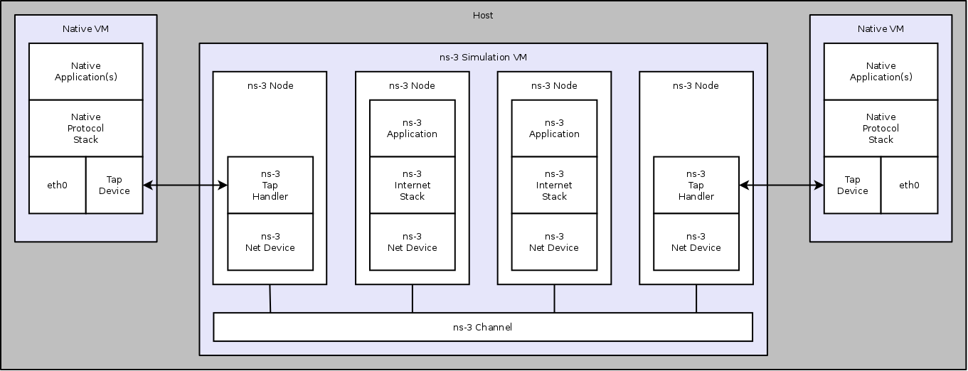
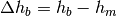
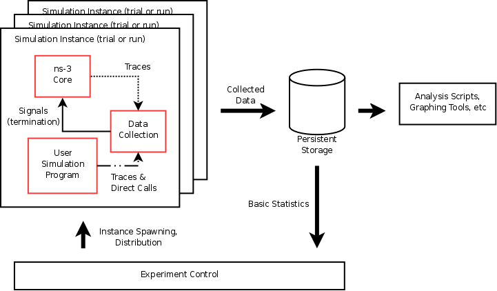
The Tap NetDevice can be used to allow a host system or virtual machines to
interact with a simulation.
TapBridge Model Overview
The Tap Bridge is designed to integrate “real” internet hosts (or more
precisely, hosts that support Tun/Tap devices) into ns-3 simulations. The
goal is to make it appear to a “real” host node in that it has an ns-3 net
device as a local device. The concept of a “real host” is a bit slippery
since the “real host” may actually be virtualized using readily available
technologies such as VMware, VirtualBox or OpenVZ.
Since we are, in essence, connecting the inputs and outputs of an ns-3 net
device to the inputs and outputs of a Linux Tap net device, we call this
arrangement a Tap Bridge.
There are three basic operating modes of this device available to users.
Basic functionality is essentially identical, but the modes are different
in details regarding how the arrangement is created and configured;
and what devices can live on which side of the bridge.
We call these three modes the ConfigureLocal, UseLocal and UseBridge modes.
The first “word” in the camel case mode identifier indicates who has the
responsibility for creating and configuring the taps. For example,
the “Configure” in ConfigureLocal mode indicates that it is the TapBridge
that has responsibility for configuring the tap. In UseLocal mode and
UseBridge modes, the “Use” prefix indicates that the TapBridge is asked to
“Use” an existing configuration.
In other words, in ConfigureLocal mode, the TapBridge has the responsibility
for creating and configuring the TAP devices. In UseBridge or UseLocal
modes, the user provides a configuration and the TapBridge adapts to that
configuration.
TapBridge UseLocal Mode
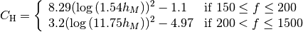
The UseLocal mode is quite similar to the ConfigureLocal mode. The
significant difference is, as the mode name implies, the TapBridge is
going to “Use” an existing tap device previously created and configured
by the user. This mode is particularly useful when a virtualization
scheme automatically creates tap devices and ns-3 is used to provide
simulated networks for those devices.
+--------+
|  Linux |
|  host  |                    +----------+
| ------ |                    |   ghost  |
|  apps  |                    |   node   |
| ------ |                    | -------- |
|  stack |                    |    IP    |     +----------+
| ------ |                    |   stack  |     |   node   |
|  TAP   |                    |==========|     | -------- |
| device | <----- IPC ------> |   tap    |     |    IP    |
| MAC X  |                    |  bridge  |     |   stack  |
+--------+                    | -------- |     | -------- |
                              |   ns-3   |     |   ns-3   |
                              |   net    |     |   net    |
                              |  device  |     |  device  |
                              |  MAC Y   |     |  MAC Z   |
                              +----------+     +----------+
                                   ||               ||
                              +---------------------------+
                              |        ns-3 channel       |
                              +---------------------------+
In this case, the pre-configured MAC address of the “Tap device” (MAC X)
will not be the same as that of the bridged “ns-3 net device” (MAC Y) shown
in the illustration above. In order to bridge to ns-3 net devices which do
not support SendFrom() (especially wireless STA nodes) we impose a requirement
that only one Linux device (with one unique MAC address – here X) generates
traffic that flows across the IPC link. This is because the MAC addresses of
traffic across the IPC link will be “spoofed” or changed to make it appear to
Linux and ns-3 that they have the same address. That is, traffic moving from
the Linux host to the ns-3 ghost node will have its MAC address changed from
X to Y and traffic from the ghost node to the Linux host will have its MAC
address changed from Y to X. Since there is a one-to-one correspondence
between devices, there may only be one MAC source flowing from the Linux side.
This means that Linux bridges with more than one net device added are
incompatible with UseLocal mode.
In UseLocal mode, the user is expected to create and configure a tap device
completely outside the scope of the ns-3 simulation using something like:
sudo tunctl -t tap0
sudo ifconfig tap0 hw ether 08:00:2e:00:00:01
sudo ifconfig tap0 10.1.1.1 netmask 255.255.255.0 up
To tell the TapBridge what is going on, the user will set either directly
into the TapBridge or via the TapBridgeHelper, the “DeviceName” attribute.
In the case of the configuration above, the “DeviceName” attribute would be
set to “tap0” and the “Mode” attribute would be set to “UseLocal”.
One particular use case for this mode is in the OpenVZ environment. There it
is possible to create a Tap device on the “Hardware Node” and move it into a
Virtual Private Server. If the TapBridge is able to use an existing tap device
it is then possible to avoid the overhead of an OS bridge in that environment.
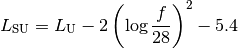
TapBridge UseBridge Mode
The simplest mode for those familiar with Linux networking is the UseBridge
mode. Again, the “Use” prefix indicates that the TapBridge is going to Use
an existing configuration. In this case, the TapBridge is going to logically
extend a Linux bridge into ns-3.
This is illustrated below:
+---------+
|  Linux  |                             +----------+
| ------- |                             |   ghost  |
|  apps   |                             |   node   |
| ------- |                             | -------- |
|  stack  |                             |    IP    |     +----------+
| ------- | +--------+                  |   stack  |     |   node   |
| Virtual | |  TAP   |                  |==========|     | -------- |
| Device  | | Device | <---- IPC -----> |   tap    |     |    IP    |
+---------+ +--------+                  |  bridge  |     |   stack  |
    ||          ||                      | -------- |     | -------- |
+--------------------+                  |   ns-3   |     |   ns-3   |
| OS (brctl) Bridge  |                  |   net    |     |   net    |
+--------------------+                  |  device  |     |  device  |
                                        +----------+     +----------+
                                             ||               ||
                                        +---------------------------+
                                        |        ns-3 channel       |
                                        +---------------------------+
In this case, a computer running Linux applications, protocols, etc., is
connected to a ns-3 simulated network in such a way as to make it appear
to the Linux host that the TAP device is a real network device participating
in the Linux bridge.
In the ns-3 simulation, a TapBridge is created to match each TAP Device.
The name of the TAP Device is assigned to the Tap Bridge using the
“DeviceName” attribute. The TapBridge then logically extends the OS bridge
to encompass the ns-3 net device.
Since this mode logically extends an OS bridge, there may be many Linux net
devices on the non-ns-3 side of the bridge. Therefore, like a net device on
any bridge, the ns-3 net device must deal with the possibly of many source
addresses. Thus, ns-3 devices must support SendFrom()
(NetDevice::SupportsSendFrom() must return true) in order to be configured
for use in UseBridge mode.
It is expected that the user will do something like the following to
configure the bridge and tap completely outside ns-3:
sudo brctl addbr mybridge
sudo tunctl -t mytap
sudo ifconfig mytap hw ether 00:00:00:00:00:01
sudo ifconfig mytap 0.0.0.0 up
sudo brctl addif mybridge mytap
sudo brctl addif mybridge ...
sudo ifconfig mybridge 10.1.1.1 netmask 255.255.255.0 up
To tell the TapBridge what is going on, the user will set either directly
into the TapBridge or via the TapBridgeHelper, the “DeviceName” attribute.
In the case of the configuration above, the “DeviceName” attribute would be
set to “mytap” and the “Mode” attribute would be set to “UseBridge”.
This mode is especially useful in the case of virtualization where the
configuration of the virtual hosts may be dictated by another system and
not be changable to suit ns-3. For example, a particular VM scheme may create
virtual “vethx” or “vmnetx” devices that appear local to virtual hosts. In
order to connect to such systems, one would need to manually create TAP devices
on the host system and brigde these TAP devices to the existing (VM) virtual
devices. The job of the Tap Bridge in this case is to extend the bridge to
join a ns-3 net device.
TapBridge ConfigureLocal Operation
In ConfigureLocal mode, the TapBridge and therefore its associated ns-3 net
device appears to the Linux host computer as a network device just like any
arbitrary “eth0” or “ath0” might appear. The creation and configuration
of the TAP device is done by the ns-3 simulation and no manual configuration
is required by the user. The IP addresses, MAC addresses, gateways, etc.,
for created TAP devices are extracted from the simulation itself by querying
the configuration of the ns-3 device and the TapBridge Attributes.
Since the MAC addresses are identical on the Linux side and the ns-3 side,
we can use Send() on the ns-3 device which is available on all ns-3 net devices.
Since the MAC addresses are identical there is no requirement to hook the
promiscuous callback on the receive side. Therefore there are no restrictions
on the kinds of net device that are usable in ConfigureLocal mode.
The TapBridge appears to an ns-3 simulation as a channel-less net device.
This device must not have an IP address associated with it, but the bridged
(ns-3) net device must have an IP address. Be aware that this is the inverse
of an ns-3 BridgeNetDevice (or a conventional bridge in general) which
demands that its bridge ports not have IP addresses, but allows the bridge
device itself to have an IP address.
The host computer will appear in a simulation as a “ghost” node that contains
one TapBridge for each NetDevice that is being bridged. From the perspective
of a simulation, the only difference between a ghost node and any other node
will be the presence of the TapBridge devices. Note however, that the
presence of the TapBridge does affect the connectivity of the net device to
the IP stack of the ghost node.
Configuration of address information and the ns-3 devices is not changed in
any way if a TapBridge is present. A TapBridge will pick up the addressing
information from the ns-3 net device to which it is connected (its “bridged”
net device) and use that information to create and configure the TAP device
on the real host.
The end result of this is a situation where one can, for example, use the
standard ping utility on a real host to ping a simulated ns-3 node. If
correct routes are added to the internet host (this is expected to be done
automatically in future ns-3 releases), the routing systems in ns-3 will
enable correct routing of the packets across simulated ns-3 networks.
For an example of this, see the example program, tap-wifi-dumbbell.cc in
the ns-3 distribution.
The Tap Bridge lives in a kind of a gray world somewhere between a Linux host
and an ns-3 bridge device. From the Linux perspective, this code appears as
the user mode handler for a TAP net device. In ConfigureLocal mode, this Tap
device is automatically created by the ns-3 simulation. When the Linux host
writes to one of these automatically created /dev/tap devices, the write is
redirected into the TapBridge that lives in the ns-3 world; and from this
perspective, the packet write on Linux becomes a packet read in the Tap Bridge.
In other words, a Linux process writes a packet to a tap device and this packet
is redirected by the network tap mechanism toan ns-3 process where it is
received by the TapBridge as a result of a read operation there. The TapBridge
then writes the packet to the ns-3 net device to which it is bridged; and
therefore it appears as if the Linux host sent a packet directly through an
ns-3 net device onto an ns-3 network.
In the other direction, a packet received by the ns-3 net device connected to
the Tap Bridge is sent via a receive callback to the TapBridge. The
TapBridge then takes that packet and writes it back to the host using the
network tap mechanism. This write to the device will appear to the Linux
host as if a packet has arrived on a net device; and therefore as if a packet
received by the ns-3 net device during a simulation has appeared on a real
Linux net device.
The upshot is that the Tap Bridge appears to bridge a tap device on a
Linux host in the “real world” to an ns-3 net device in the simulation.
Because the TAP device and the bridged ns-3 net device have the same MAC
address and the network tap IPC link is not externalized, this particular
kind of bridge makes it appear that a ns-3 net device is actually installed
in the Linux host.
In order to implement this on the ns-3 side, we need a “ghost node” in the
simulation to hold the bridged ns-3 net device and the TapBridge. This node
should not actually do anything else in the simulation since its job is
simply to make the net device appear in Linux. This is not just arbitrary
policy, it is because:
- Bits sent to the TapBridge from higher layers in the ghost node (using
the TapBridge Send method) are completely ignored. The TapBridge is
not, itself, connected to any network, neither in Linux nor in ns-3. You
can never send nor receive data over a TapBridge from the ghost node.
- The bridged ns-3 net device has its receive callback disconnected
from the ns-3 node and reconnected to the Tap Bridge. All data received
by a bridged device will then be sent to the Linux host and will not be
received by the node. From the perspective of the ghost node, you can
send over this device but you cannot ever receive.
Of course, if you understand all of the issues you can take control of
your own destiny and do whatever you want – we do not actively
prevent you from using the ghost node for anything you decide. You
will be able to perform typical ns-3 operations on the ghost node if
you so desire. The internet stack, for example, must be there and
functional on that node in order to participate in IP address
assignment and global routing. However, as mentioned above,
interfaces talking to any TapBridge or associated bridged net devices
will not work completely. If you understand exactly what you are
doing, you can set up other interfaces and devices on the ghost node
and use them; or take advantage of the operational send side of the
bridged devices to create traffic generators. We generally recommend
that you treat this node as a ghost of the Linux host and leave it to
itself, though.
TapBridge UseLocal Mode Operation
As described in above, the TapBridge acts like a bridge from the “real” world
into the simulated ns-3 world. In the case of the ConfigureLocal mode,
life is easy since the IP address of the Tap device matches the IP address of
the ns-3 device and the MAC address of the Tap device matches the MAC address
of the ns-3 device; and there is a one-to-one relationship between the
devices.
Things are slightly complicated when a Tap device is externally configured
with a different MAC address than the ns-3 net device. The conventional way
to deal with this kind of difference is to use promiscuous mode in the
bridged device to receive packets destined for the different MAC address and
forward them off to Linux. In order to move packets the other way, the
conventional solution is SendFrom() which allows a caller to “spoof” or change
the source MAC address to match the different Linux MAC address.
We do have a specific requirement to be able to bridge Linux Virtual Machines
onto wireless STA nodes. Unfortunately, the 802.11 spec doesn’t provide a
good way to implement SendFrom(), so we have to work around that problem.
To this end, we provided the UseLocal mode of the Tap Bridge. This mode allows
you approach the problem as if you were creating a bridge with a single net
device. A single allowed address on the Linux side is remembered in the
TapBridge, and all packets coming from the Linux side are repeated out the
ns-3 side using the ns-3 device MAC source address. All packets coming in
from the ns-3 side are repeated out the Linux side using the remembered MAC
address. This allows us to use Send() on the ns-3 device side which is
available on all ns-3 net devices.
UseLocal mode is identical to the ConfigureLocal mode except for the creation
and configuration of the tap device and the MAC address spoofing.
TapBridge UseBridge Operation
As described in the ConfigureLocal mode section, when the Linux host writes to
one of the /dev/tap devices, the write is redirected into the TapBridge
that lives in the ns-3 world. In the case of the UseBridge mode, these
packets will need to be sent out on the ns-3 network as if they were sent on
a device participating in the Linux bridge. This means calling the
SendFrom() method on the bridged device and providing the source MAC address
found in the packet.
In the other direction, a packet received by an ns-3 net device is hooked
via callback to the TapBridge. This must be done in promiscuous mode since
the goal is to bridge the ns-3 net device onto the OS (brctl) bridge of
which the TAP device is a part.
For these reasons, only ns-3 net devices that support SendFrom() and have a
hookable promiscuous receive callback are allowed to participate in UseBridge
mode TapBridge configurations.


 which is the location
of the antenna, and then transforming the coordinates of every generic
point
which is the location
of the antenna, and then transforming the coordinates of every generic
point  of the space from cartesian coordinates
 into spherical coordinates
 .
The antenna model neglects the radial component
.
The antenna model neglects the radial component  , and
only considers the angle components
, and
only considers the angle components  . An antenna
radiation pattern is then expressed as a mathematical function
. An antenna
radiation pattern is then expressed as a mathematical function
 that returns the
gain (in dB) for each possible direction of
transmission/reception. All angles are expressed in radians.
that returns the
gain (in dB) for each possible direction of
transmission/reception. All angles are expressed in radians.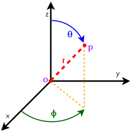
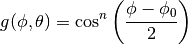
 is the azimuthal orientation of the antenna
(i.e., its direction of maximum gain) and the exponential
is the azimuthal orientation of the antenna
(i.e., its direction of maximum gain) and the exponential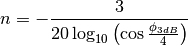
 .
.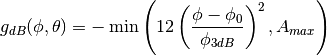
 is the maximum attenuation in dB of the
antenna.
is the maximum attenuation in dB of the
antenna. determied by the constructor to known reference values. The test
passes if for each case the values are equal to the reference up to a
tolerance of
determied by the constructor to known reference values. The test
passes if for each case the values are equal to the reference up to a
tolerance of  which accounts for numerical errors.
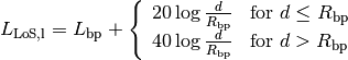
![L_\mathrm{total} = 20\log f + N\log d + L_f(n)- 28 [dB]](_images/math/813059cb5c7dede10dfb9daf3503723ace601eca.png)
 : power loss coefficient [dB]
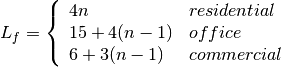
 : number of floors between base station and mobile (
 )
) : frequency [MHz]
 : distance (where
  ) [m]
) [m] , and approximating the number of walls that are penetrated with the manhattan distance (in number of rooms) between the transmitter and the receiver. In detail, let
  ,
,  ,
,  ,
,  denote the room number along the
  and
and  axis respectively for user 1 and 2; the total loss
  is calculated as
 .
. .
.
 ) has to be calculated as the square root of the sum of the quadratic values of the standard deviatio in case of outdoor nodes and the one for the external walls penetration. This is due to the fact that that the components producing the shadowing are independent of each other; therefore, the variance of a distribution resulting from the sum of two independent normal ones is the sum of the variances.
 and variable standard deviation
  , according to models commonly used in literature.
The test generates 10,000 samples of shadowing by subtracting the deterministic component from the total loss returned by the
, according to models commonly used in literature.
The test generates 10,000 samples of shadowing by subtracting the deterministic component from the total loss returned by the 
 denote the
generic user, and let
denote the
generic user, and let  be its SINR. We get the spectral efficiency
 of user
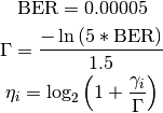
 denote generic users; let
  be the
subframe index, and
be the
subframe index, and  be the resource block index; let
  be MCS
usable by user
be MCS
usable by user  be the TB
size in bits as defined in
be the TB
size in bits as defined in  of
resource blocks is used. The achievable rate
of
resource blocks is used. The achievable rate  in bit/s for user
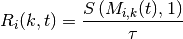
 is the TTI duration.
At the start of each subframe
is the TTI duration.
At the start of each subframe  to which RBG
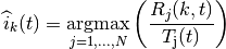
 is the past througput performance perceived by the
user
is the past througput performance perceived by the
user  .
According to the above scheduling algorithm, a user can be allocated to
different RBGs, which can be either adjacent or not, depending on the current
condition of the channel and the past throughput performance
.
According to the above scheduling algorithm, a user can be allocated to
different RBGs, which can be either adjacent or not, depending on the current
condition of the channel and the past throughput performance 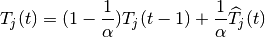
 is the time constant (in number of subframes) of
the exponential moving average, and
is the time constant (in number of subframes) of
the exponential moving average, and  is the actual
throughput achieved by the user
is the actual
throughput achieved by the user  actually used by user
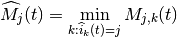
 of RBGs allocated to user
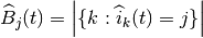
 indicates the cardinality of the set; finally,
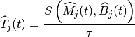
 denote the LTE Absolute Radio Frequency Channel Number, which
identifies the carrier frequency on a 100 kHz raster; furthermore, let
denote the LTE Absolute Radio Frequency Channel Number, which
identifies the carrier frequency on a 100 kHz raster; furthermore, let  used in the simulation we define a corresponding spectrum
model using the Spectrum framework described
in
used in the simulation we define a corresponding spectrum
model using the Spectrum framework described
in 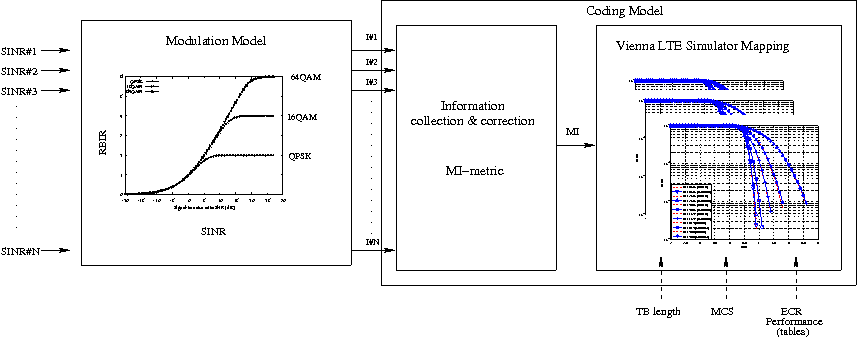
 blocks of size
  and
and  blocks of size
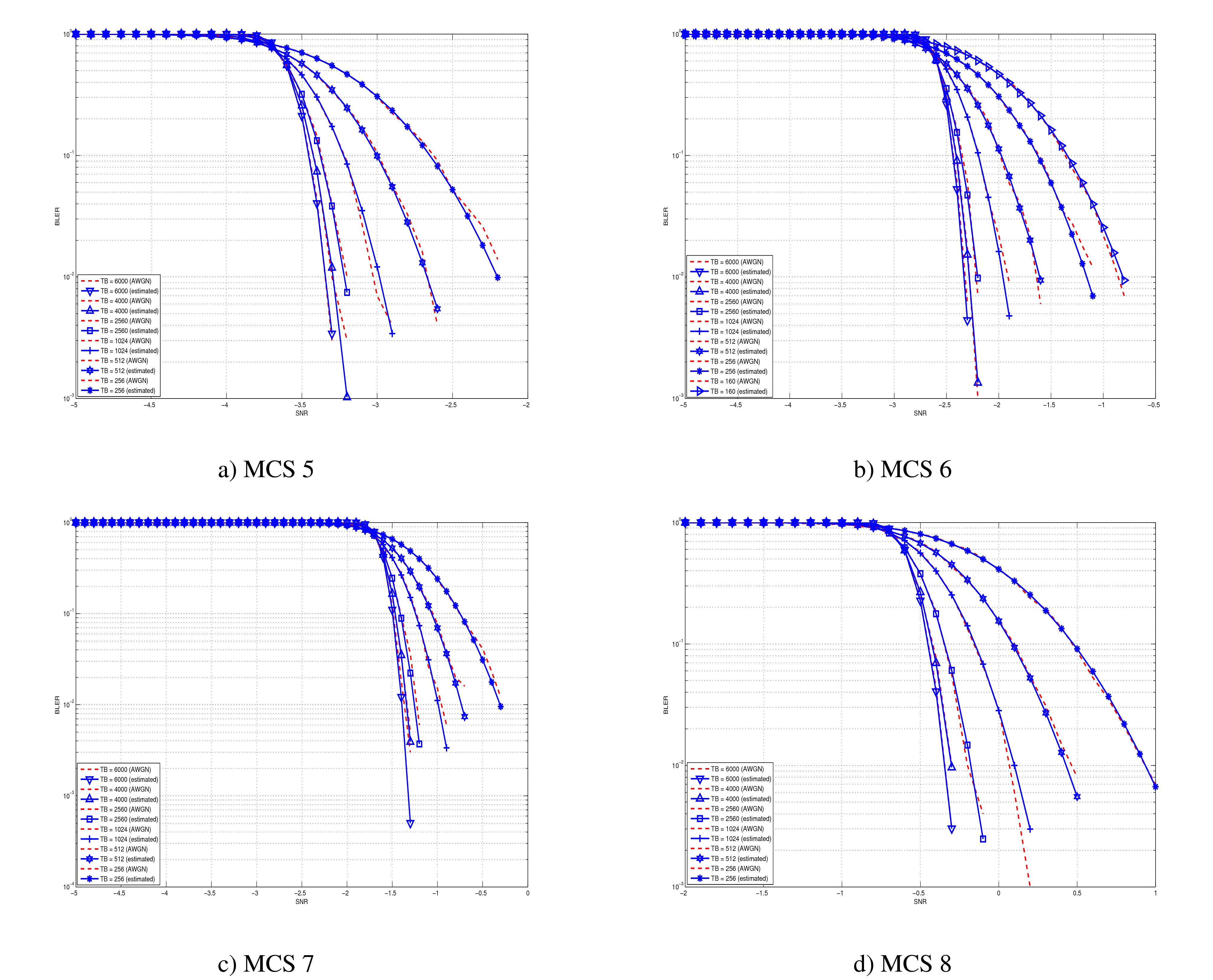
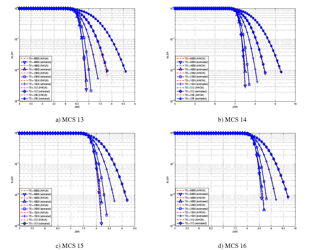
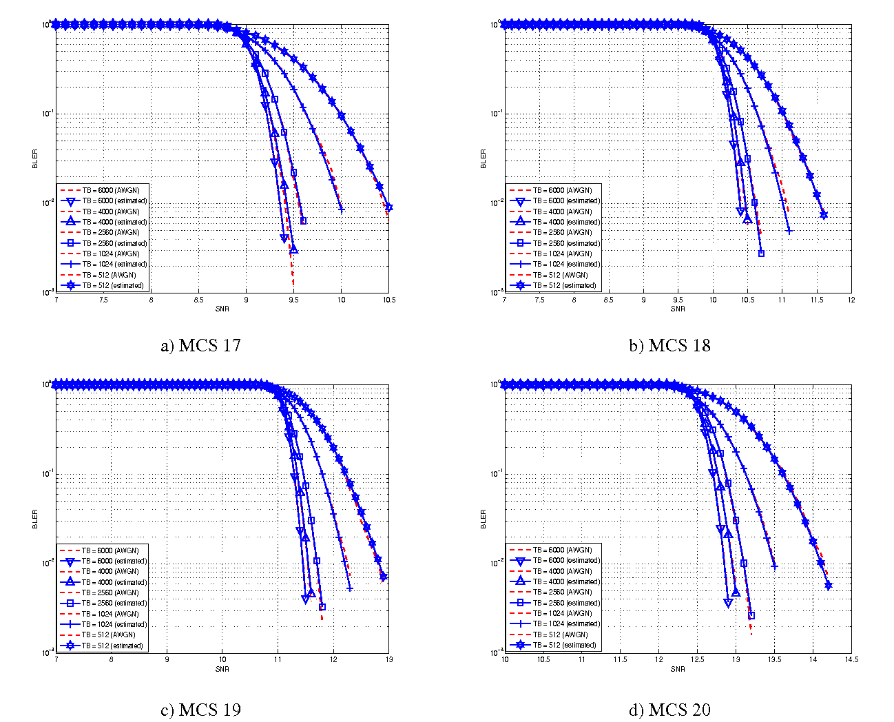
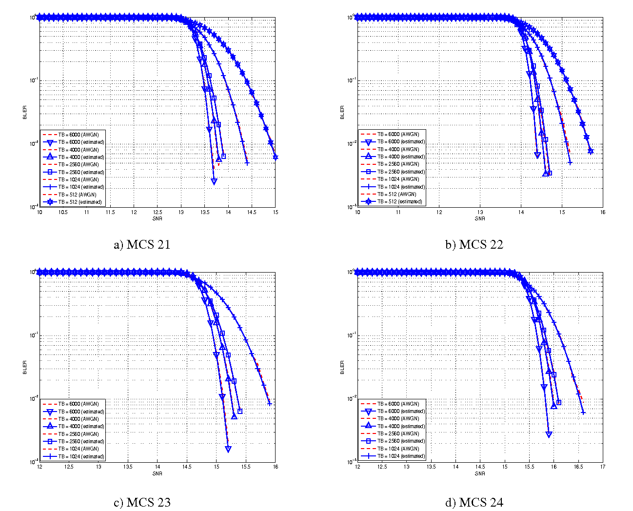
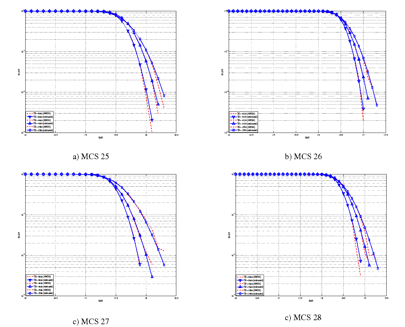
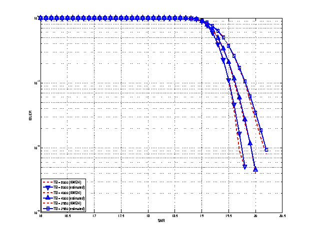
  . Therefore the overall TB BLER (TBLER) can be expressed as
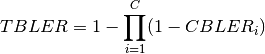
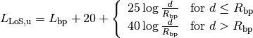
 is the BLER of the CB
 ![CBLER_i = \frac{1}{2}\left[1-erf\left(\frac{x-b_{ECR}}{\sqrt{2}c_{ECR}} \right) \right]](_images/math/c67a23d92ea8d111d9b02d8a7610388a7074b054.png)
 represents the “transition center” and
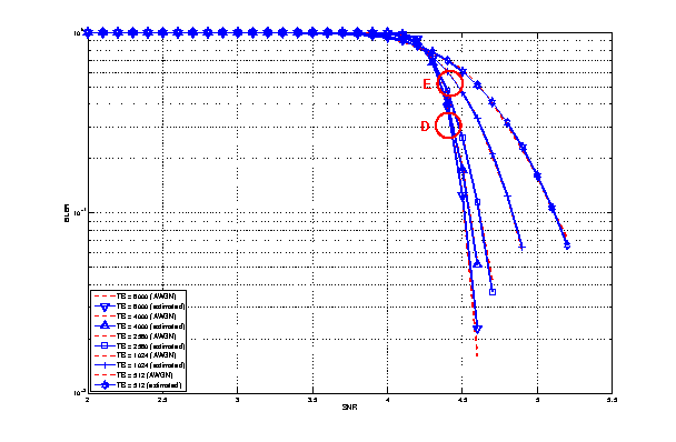
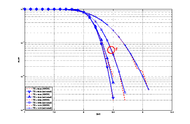
  is related to the “transition width” of the Gaussian cumulative distribution for each Effective Code Rate (ECR) which is the actual transmission rate according to the channel coding and MCS. For limiting the computational complexity of the model we considered only a subset of the possible ECRs in fact we would have potentially 5076 possible ECRs (i.e., 27 MCSs and 188 CB sizes). On this respect, we will limit the CB sizes to some representative values (i.e., 40, 140, 160, 256, 512, 1024, 2048, 4032, 6144), while for the others the worst one approximating the real one will be used (i.e., the smaller CB size value available respect to the real one). This choice is aligned to the typical performance of turbo codes, where the CB size is not strongly impacting on the BLER. However, it is to be notes that for CB sizes lower than 1000 bits the effect might be relevant (i.e., till 2 dB); therefore, we adopt this unbalanced sampling interval for having more precision where it is necessary. This behaviour is confirmed by the figures presented in the Annes Section.
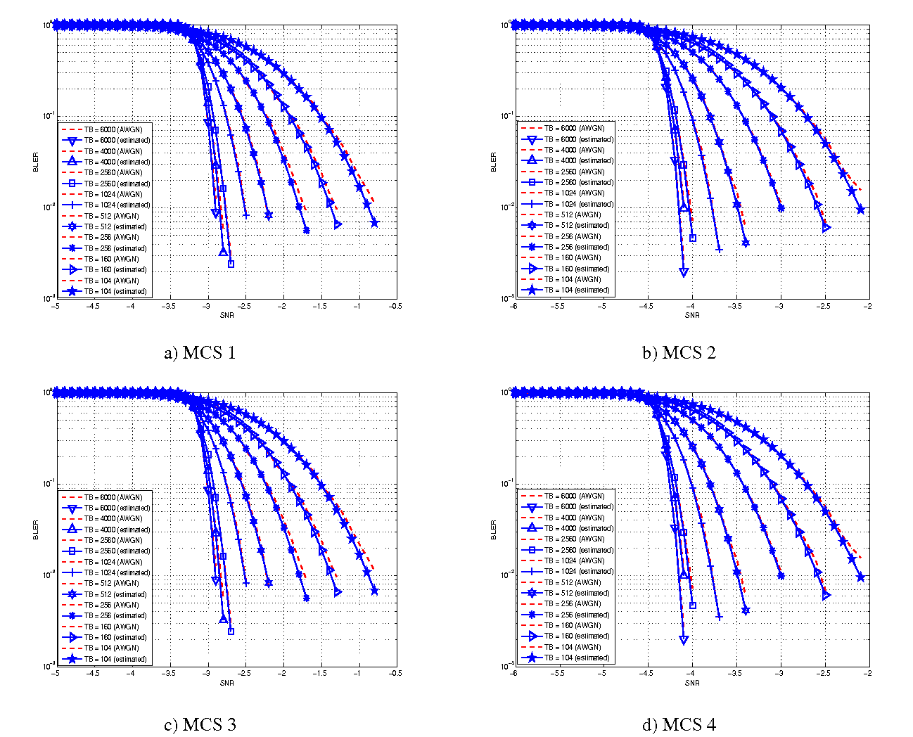
 and
and  [dB].
[dB]. and
and  [dB].
[dB]. and
and  [dB].
[dB]. and
and  [dB].
[dB]. and
and  [dB].
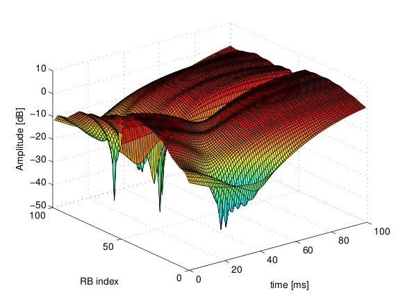
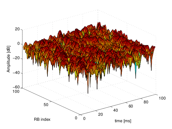
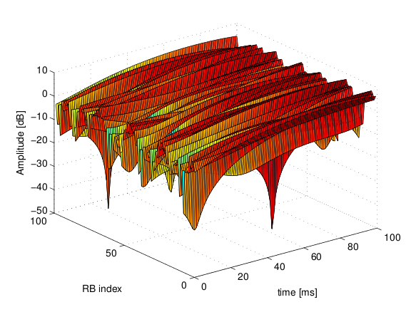
[dB]. of the fading traces:
![S_{traces} = S_{sample} \times N_{RB} \times \frac{T_{trace}}{T_{sample}} \times N_{scenarios} \mbox{ [bytes]}](_images/math/ae405135ea7b6d064554d9157ab14f83d706ba70.png)
 is the size in bytes of the sample (e.g., 8 in case of double precision, 4 in case of float precision),
  is the number of RB or set of RBs to be considered,
  is the total length of the trace,
  is the time resolution of the trace (1 ms), and
  is the number of fading scenarios that are desired (i.e., combinations of different sets of channel taps and user speed values). We provide traces for 3 different scenarios one for each taps configuration defined in Annex B.2 of
  . All traces have
  s and
s and  . This results in a total 24 MB bytes of traces.
 degrees from the direction of orientation is -3 dB.
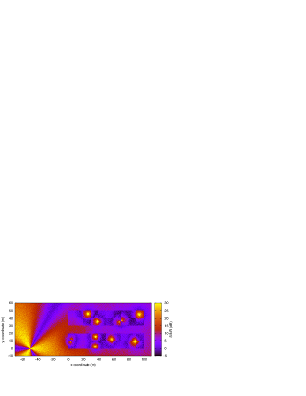
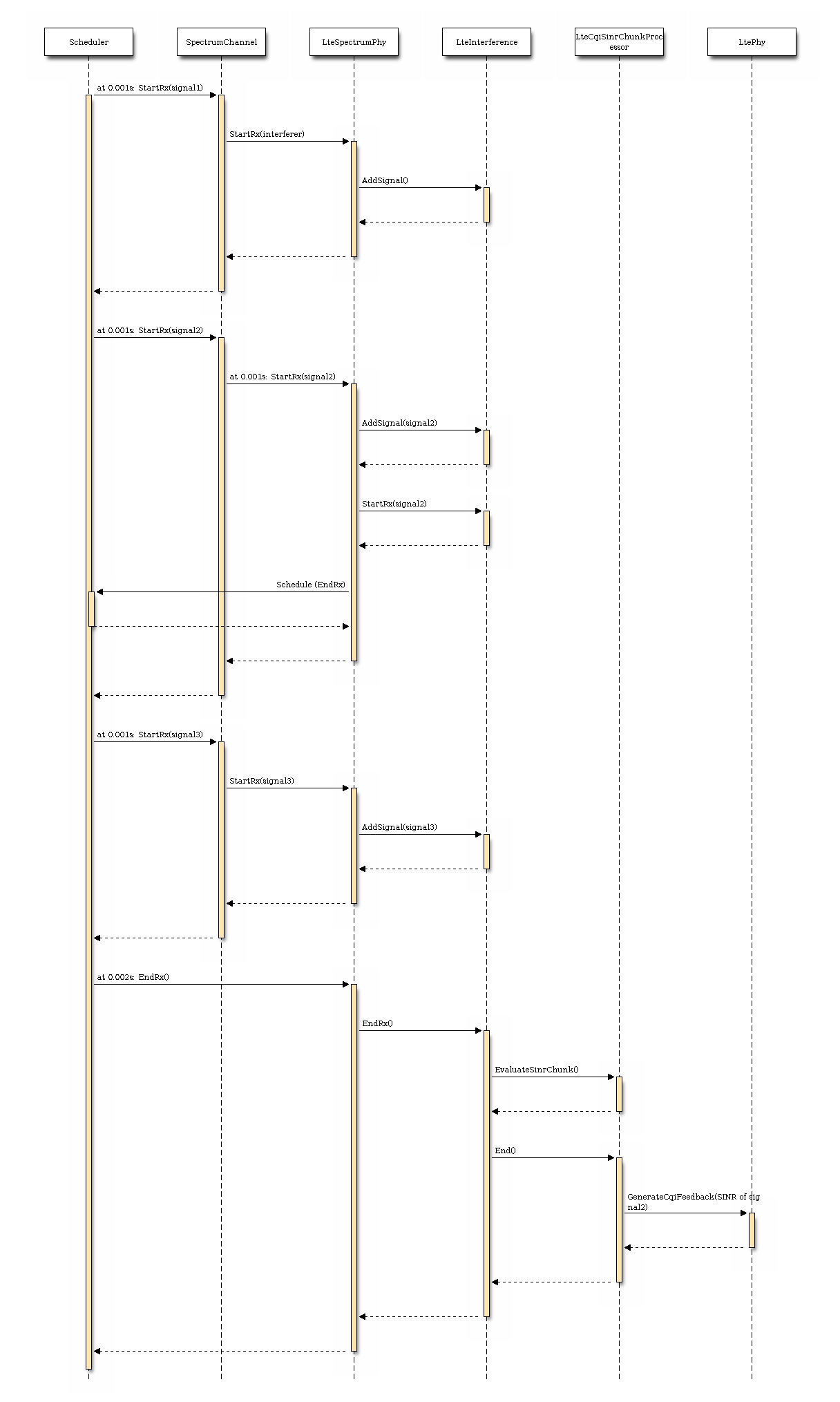
 its duration and
  its SINR,
calculated with the above equation. The calculation of the average
SINR
its SINR,
calculated with the above equation. The calculation of the average
SINR  to be used for CQI feedback reporting
uses the following formula:
to be used for CQI feedback reporting
uses the following formula:
 . The tolerance is meant to account for
the approximation errors typical of floating point arithmetic.
. The tolerance is meant to account for
the approximation errors typical of floating point arithmetic.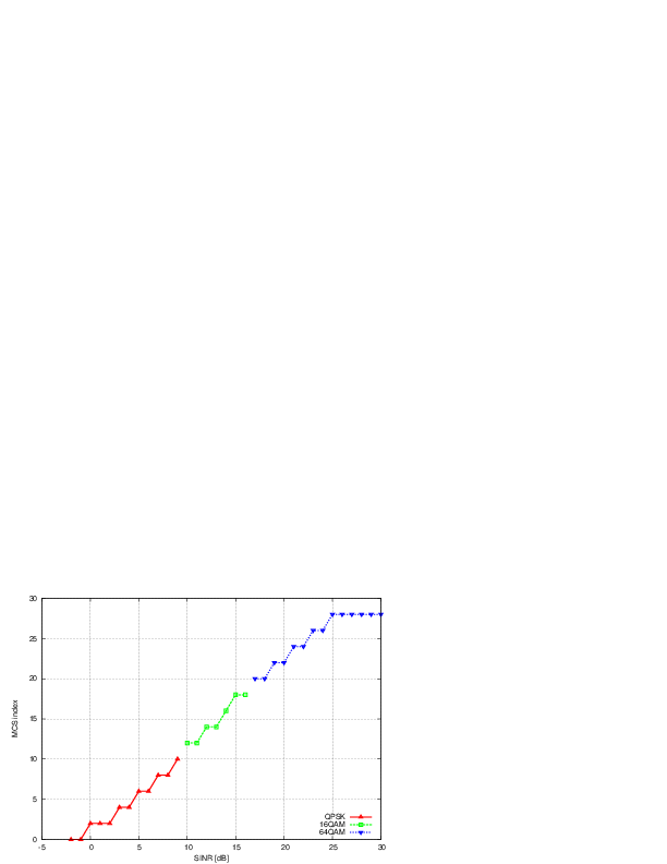
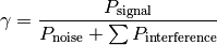
 parameter represents the distance of each UE to the eNB it
is attached to, whereas the
parameter represents the distance of each UE to the eNB it
is attached to, whereas the  parameter represent the
interferer distance. We note that the scenario topology is such that
the interferer distance is the same for uplink and downlink; still,
the actual interference power perceived will be different, because of
the different propagation loss in the uplink and downlink
bands. Different test cases are obtained by varying the
parameter represent the
interferer distance. We note that the scenario topology is such that
the interferer distance is the same for uplink and downlink; still,
the actual interference power perceived will be different, because of
the different propagation loss in the uplink and downlink
bands. Different test cases are obtained by varying the 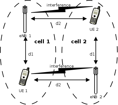
 be the
number of UEs,
be the
number of UEs,  the RBG size,
  the modulation and
coding scheme in use at the given SINR and
the modulation and
coding scheme in use at the given SINR and  of RBGs allocated to each user as
 in bit/s achieved by each UE is then calculated as
 be the modulation and coding scheme being used by
each UE (which is a deterministic function of the SINR of the UE, and is hence
known in this scenario). Based on the MCS, we determine the achievable
rate
be the modulation and coding scheme being used by
each UE (which is a deterministic function of the SINR of the UE, and is hence
known in this scenario). Based on the MCS, we determine the achievable
rate  for each user
  of each user
 of UE
of UE 


 is a constant. By substituting the above into the
definition of
is a constant. By substituting the above into the
definition of 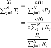
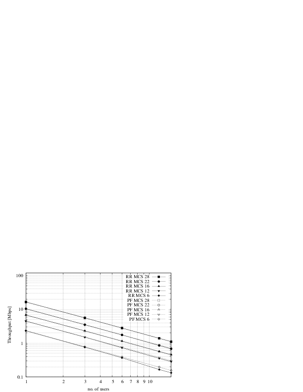
 that are located at a distance from the base
station such that they will use respectively the MCS index
that are located at a distance from the base
station such that they will use respectively the MCS index  . From the figure, we note that, as expected, the obtained throughput is
proportional to the achievable rate. In other words, the PF scheduler assign
more resources to the users that use a higher MCS index.
. From the figure, we note that, as expected, the obtained throughput is
proportional to the achievable rate. In other words, the PF scheduler assign
more resources to the users that use a higher MCS index.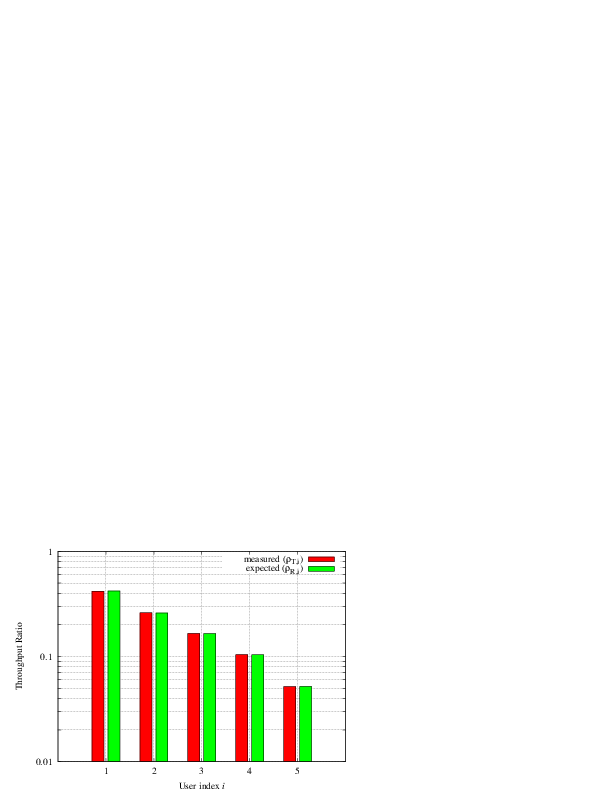
 dB, which accouns for numerical
errors in the calculations.
dB, which accouns for numerical
errors in the calculations.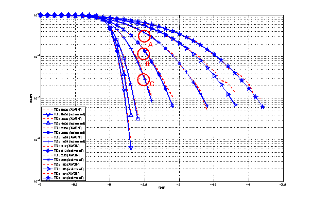
 , the parameter
  which accounts for numerical errors.
Different test cases are provided by varying the x and y coordinates
of the UE, and the beamwidth and the orientation of the antenna of
the eNB.
which accounts for numerical errors.
Different test cases are provided by varying the x and y coordinates
of the UE, and the beamwidth and the orientation of the antenna of
the eNB.


 : eNB height above the ground [m]
 : UE height above the ground [m]
 : is a logarithm in base 10 (this for the whole document)

 : pathloss in urban areas
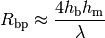
 : wavelength [m]
 : UE height above the ground [m]
 is the value for the basic transmission loss at the break point, defined as:
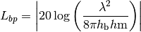
 ), the diffraction loss from rooftop to street (
 ) and the reduction due to multiple screen diffraction past rows of building (
 ). The formula is:
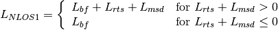

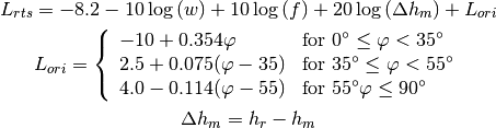
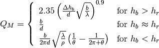
 : is the height of the rooftop [m]
 : is the height of the mobile [m]
 : is the street orientation with respect to the direct path (degrees)
 (where l is the distance over which the building extend), it can be evaluated according to
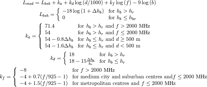
 , the formula is:
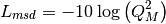
 , the reference distance,
 is choosen equal to
  and the reference energy is based
based on a Friis propagation model.
and the reference energy is based
based on a Friis propagation model.